Train track complex of once-punctured torus and 4-punctured sphere
Abstract.
Consider a compact oriented surface of genus and punctured. The train track complex of which is defined by Hamenstädt is a 1-complex whose vertices are isotopy classes of complete train tracks on . Hamenstädt shows that if , the mapping class group acts properly discontinuously and cocompactly on the train track complex. We will prove corresponding results for the excluded case, namely when is a once-punctured torus or a 4-punctured sphere. To work this out, we redefinition of two complexes for these surfaces.
Key words and phrases:
Mapping class group, Train track, Curve complex2000 Mathematics Subject Classification
57M601. Introduction
Consider a compact oriented surface of genus from which points, so-called punctures, have been deleted. The mapping class group of is, by definition, the space of isotopy classes of orientation preserving homeomorphisms of .
There are natural metric graphs on which the mapping class group acts by isometries. Among them, we will concern with the curve complex (or, rather, its one-skeleton) and train track complex .
In [Har81], Harvey defined the curve complex for . The vertex of this complex is a free homotopy class of an essential simple closed curve on , i.e. a simple closed curve which is neither contractible nor homotopic into a puncture. A -simplex of is spun by a collection of vertices which are realized by mutually disjoint simple closed curves.
The train track which is an embedded 1-complex was invented by Thurston [Thu78] and provides a powerful tool for the investigation of surfaces and hyperbolic -manifolds. A detailed account on train tracks can be found in the book [Pen92] of Penner with Harer.
Hamenstädt defined in [Ham05a] that a train track is called complete if it is a bireccurent and each of complementary regions is either a trigon or a once-punctured monogon. Hamenstädt defined the train track complex for . Vertices of the train track complex are isotopy classes of complete train tracks on .
Suppose , i.e. S is a hyperbolic surfaces but neither a once-punctured torus nor 4-punctured sphere. Both the curve complex and the train track complex can be endowed with a path-metric by declaring all edge lengths to be equal to 1. In these cases, there are a map and a number such that for all complete train track on .
If is a once-punctured torus or a 4-punctured sphere, then any essential simple closed curve must intersect, so that has no edge by definition. However, Minsky [Min96] adopt a small adjustment in the definition for curve complex in these two particular case so that it becomes a sensible and familiar 1-complex: two vertices are connected by an edge when the curves they represent have minimal intersection (1 in the case of a once-punctured torus, and 2 in the case of a 4-punctured sphere). It turns out that in both cases, the complex is the Farey graph .
In addition, if is a once-punctured torus, there is no complete train track under Hamenstädt’s definition and is homeomorphic to empty set. We thus adopt here Penner’s definition [Pen92], i.e. the train track is complete iff is bireccurent and is not a proper subtrack of any birecurrent train track. These two definitions are equivalent except for the once-punctured torus.
Our main theorem is:
Theorem 1.1.
Suppose is a once-punctured torus or a 4-punctured sphere. Then the train track complex of is quasi-isometric to the dual graph of the Farey graph (see Figure1).

More precisely, if is a once-punctured torus, we show:
Theorem 1.2.
The train track complex of a once-punctured torus is isomorphic to the Caley graph of .
In [Ham05a], Hamenstädt also shows that if the mapping class group acts p.d.c., i.e. properly discontinuously and cocompactly, on the train track complex and is quasi-isometric to . We can prove that the same is true for the once-punctured torus and 4-punctured sphere.
Corollary 1.3.
Suppose is the once-punctured torus or 4-punctured sphere. Then acts p.d.c. on .
Corollary 1.4.
Suppose is the once-punctured torus or 4-punctured sphere. Then is quasi-isometric to .
In Section 2, we give a brief review of quasi-isometries. In Section 3, we describe train tracks and define the train track complex. In Section 4, we describe how to build a Farey graph which is used for curve complex of a once-punctured torus or a 4-punctured sphere. In Section 5 and 6, we prove the Theorem1.1. Finally, we describe the action of mapping class groups on train track complexes in Section 7.
2. Quasi-Isometry
A quasi-isometry is one of the fundamental notion in geometric group theory. For details, see [Bow06].
Let be a proper geodesic space, i.e. a complete and locally compact geodesic space. Given and , write for the closed -neighborhood of in . If , write . We say that is cobounded if for some .
Suppose that a group acts on X by isometry. Given , we write for the orbit of under , and for its stabilizer.
We say that the action of on is properly discontinuous if for all and all , the set is finite. A properly discontinuous action is called cocompact if is compact. We will frequently abbreviate “properly discontinuous and cocompact” by p.d.c.
Proposition 2.1 ([Bow06]).
The followings are equivalent:
- (i)
The action is cocompact,
- (ii)
Some orbit is cobounded, and
- (iii)
Every orbit is cobounded.
Proof.
Write for a closed -neighborhood of in . Let be a quotient map, Then for any and any and .
- •
(iii) (ii) is clear.
- •
Suppose that some orbit is cobounded. So, for some and some . Thus, . By Proposition 3.1 of [Bow06], is compact and hence is also compact. Now we proved (ii) (i).
- •
Suppose the action is cocompact. So, is compact and hence is bounded. Thus, for any there is some , such that . Since , is cobounded and (i) (iii) is shown.
∎
Definition 2.2 (quasi-isometry).
Let and be metric spaces. A map is called a quasi-isometry if there are constants such that for all ,
and the image is cobounded in .
Thus, a quasi-isometry is bi-Lipshitz with bounded error and its image is cobounded. We note that the quasi-isometry introduces an equivalence relation on the set of metric spaces.
Two metric spaces, and , are said to be quasi-isometric if there is a quasi-isometry between them.
Let be a geodesic space and a finite generating set for a group . Suppose is the Cayley graph of with respect to . If is another generating set for , then is quasi-isometric to . Thus, we simply denote the Cayley graph of by without specifying a generating set. A group acts p.d.c. on its Cayley graph .
We define that is quasi-isometric to if is quasi-isometric to . Also, two groups , are quasi-isometric if is quasi-isometric to .
The proof of the following claims can be found for example in [Bow06]:
Theorem 2.3 ([Bow06]).
If acts p.d.c. on a proper geodesic space , then is quasi-isometric to .
Proposition 2.4.
Let be a finitely generated group. Suppose that is a subgroup of of finite index. Then is finitely generated and quasi-isometric to .
3. Train track complex
A train track on (see [Pen92]) is an embedded 1-complex whose vertecis are called switches and edges are called branches. is away from its switches. At any switch the incident edges are mutually tangent and there is an embedding with which is a map into . The valence of each switch is at least , except possibly for one bivalent switch in a closed curve component. Finally, we require that every component of has negative generalized Euler characteristic in the following sense: define to be the Euler characteristic minus for every outward-pointing cusp (internal angle ). For the train track complementary regions all cusps are outward, so that the condition excludes annuli, once-punctured disks with smooth boundary, or non-punctured disks with or cusps at the boundary. We will usually consider isotopic train-tracks to be the same.
A train track is called generic if all switches are at most trivalent. A train route is a non-degenerate smooth path in ; in particular it traverses a switch only by passing from incoming to outgoing edge or vice versa. The train track is called recurrent if every branch is contained in a closed train route. The train track is called transversely recurrent if every branch intersects transversely with a simple closed curve so that does not contain an embedded bigon, i.e. a disc with two corners. A train track which is both recurrent and transversely recurrent is called birecurrent.
A curve is carried by a transversely recurrent train track if there is a carrying map of class which is homotopic to the identity and maps to in such a way that the restriction of its differential to every tangent line of is non-singular. A train track is carried by if there is a carrying map and every train route on is carried by with .
A generic birecurrent train track is called complete if it is not a proper subtrack of any birecurrent train track.
Theorem 3.1 ([Pen92]).
- (i)
If or , then any birecurrent train track on is a subtrack of a complete train track, each of whose complementary region is either a trigon or a once-punctured monogon.
- (ii)
Any birecurrent train track on a once-punctured torus is a subtrack of a complete train track whose unique complementary region is a once-punctured bigon.
It follows:
Corollary 3.2.
Suppose is a complete train track on of genus with punctures. Then the number of switches of depends only on the topological type of .
Proof.
If is the once-punctured torus, then have 2 vertices.
In the other case, let be the number of triangle component of , be the number of switches of and be the number of branches of . Since is generic, . By Theorem 3.1, . By Euler characteristic, . Now we get . ∎
A half-branch in a generic train track incident on a switch is called large if the switch is trivalent and if every arc of class which passes through meets the interior of . A branch in is called large if each of its two half-branches is large; in this case is necessarily incident to two distinct switches.
There is a simple way to modify a complete train track to another complete train track. Namely, if is a large branch of then we can perform a right or left split of at as shown in Figure 2. A complete train track can always be at least one of the left or right split at any large branch to a complete train track (see [Ham05b]). We note that is carried by .
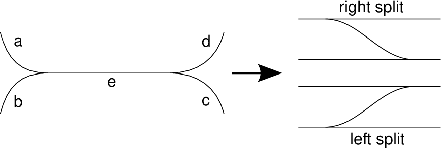
Definition 3.3 (train track complex).
A train track complex is defined as follow: The set of vertices of consists of all isotopy classes of complete train tracks on . Two Complete train tracks is connected with an edge if can be obtained from by a single split.
For each switch of , fix a direction of the tangent line to at . The branch which is incident to is called incoming if the direction at coincides with the direction from to , and outgoing if not. A transverse measure on is a non-negative function on the set of branches satisfying the switch condition : For any switch of the sums of over incoming and outgoing branches are equal. A train track is recurrent if and only if it supports a transverse measure which is positive on every branch (see [Pen92]).
For a recurrent train track the set of all transverse measures on is a convex cone in a linear space. A vertex cycle (see [MM99]) on is a transverse measure which spans an extremal ray in . Up to scaling, a vertex cycle is a counting measure of a simple closed curve which is carried by . This means that for a carrying map and every open branch of the -weight of equals the number of connected components of . We also use the notion, a vertex cycle, for the simple closed curve .
Proposition 3.4 ([Ham05b]).
Let be a complete train track. Suppose is a vertex cycle on with a carrying map . Then, passes through every branch of at most twice, and with different orientation if any.
Proposition 3.4 and Corollary 3.2 imply that the number of vertex cycles on a complete train track on is bounded by a universal constant (see [MM99]). Moreover, there is a number with the property that for every complete train track on the distance in between any two vertex cycles on is at most (see [Ham05b], [MM04]).
4. Farey graph
Let S be the once-punctured torus or the 4-punctured sphere. The essential simple closed curves on S are well known to be in one-to-one correspondence with rational numbers with Thus the -skeleton of is identified with in the circle .
There are numerous ways to build a Farey graph , any of them produces an isomorphic graph. One can start with the rational projective line , identifying with and with , and take this to be the vertex set of . Then, two projective rational numbers , where and are coprime and and are coprime, are deemed to span an edge, or 1-simplex, if and only if . The result is a connected graph in which every edge separates. The graph can be represented on a disc; see Figure 3.

We shall say a graph is a Farey graph if it is isomorphic to .
Note that the curve complexes of a once-punctured torus and 4-punctured sphere are Farey graphs (see [Min96][APS06]).
Remark.
The Farey graph is quasi-isometric to the dual graph.
5. Train tracks on the once-punctured torus
Let be the once-punctured torus and a complete train track on . By Theorem 3.1 and Corollary 3.2, has the unique complementary region that is a once-punctured bigon and the number of switches of equals 2. It follows that every complete train track on is orientation preserving –diffeomorphic to the one illustrated in Figure 4.

has exactly two vertex cycles whose intersection number equals . Thus, and is connected by an edge in Farey graph. Conversely, if we fix simple closed curve on whose intersection number equals , then there is only two complete train tracks whose vertex cycles are and .
Write for the vertex set of a graph and for the set of all edges in G. We define a map as follow: Let . Suppose are vertex cycles on . We define as the edge of which connects and .
We construct the graph of as follows: Let . We connect vertices if some and some are connected by an edge in . can be naturally extended to .
Lemma 5.1.
is quasi-isometric to the dual graph of the Farey graph.
Proof.
Suppose and are different complete train tracks on which have common vertex cycles . have a unique large edge and there are two complete train tracks which are obtained by a left or right split of at (see Figure 5).

We can see that one vertex cycle on is the same as on , and the other vertex cycle on intersects on at one point. Thus and are adjacent edges in . In this case, vertex cycles on are and . Hence , and span a triangle on . Similarly, we can get complete train tracks by a split of , and , and span another triangle on . (see Figure 7)
The mapping class group acts isometrically on and and acts transitively on . It follows that every edge in connects an adjacent edge of and every adjacent edge of is connected with a direct edge in . Thus is the line graph of the dual of , i.e. vertices of represent edges of the dual of and two vertices are adjacent iff their corresponding edges share a common endpoint (see Figure 7). It’s now obvious that is quasi-isometric to the dual of the Farey graph. ∎


Lemma 5.2.
is connected.
Proof.
Let and . All we need is to show that and are connected in , since is connected. can be a right(left) split to a complete train track . Then, there is a complete train track which can be a right(left) split to and can be a left(right) split to (see Figure 8). Thus and are connected and .

∎
Lemma 5.3.
is a quasi-isometory.
Proof.
Let . Suppose is geodesic on from to . and since for any . Thus .
It follows that is a quasi-isometry. ∎
Proof of Theorem 1.1(a once-puncture torus case).
is obtained by extending one vertex of to two vertices. When we think the action of the mapping class group, we see that is isomorphic to the graph as in Figure 9. We can notice that this graph is isomorphic to the Caley graph of , and thus Theorem 1.2 is proved.

6. Train tracks on the 4-punctured sphere
Let be the 4-punctured sphere. A train track complex of is similar to that of the once-punctured torus but more complicated.
Orientation preserving –diffeomorphism classes of a complete train tracks depends on combination of switches and branches. By Proposition 3.2, number of switches and branches of are constants. Thus, number of orientation preserving –diffeomorphism classes of the complete train tracks is finite. In fact, complete train tracks on are classified into 13 classes, illustrated in (1) to (8) of Figure 10 and their mirror images, though (1), (4) and (8) can move these mirrors by orientation preserving -diffeomorphism.

We can see that all of those train tracks have exactly two vertex cycles whose intersection number equals or .
First, we confirm connectivity of :
Proposition 6.1.
is connected.
First we look at a –diffeomorphism class which has two large edges and whose two vertex cycles intersect at two points ( (1) of Figure 10 ). We write for the collection of these train tracks.
Let . can split at two large edges , . We can get another complete train track by a right split at ( is –diffeomorphic to (2) of Figure 10). can be right split at to a complete train track , and we can find that . Incidentally, if we left split at , we cannot get a complete train track (see Figure 11). In the same way, we can get by being left splits at both and . That is to say, we can get two complete train tracks by splits at both and of .

We construct graph as follow: is . We connect by an edge if can be obtained by splits at two larges edges of . Clearly, is homeomorphic to subgraph of .
Lemma 6.2.
is connected and is quasi-isometric to the dual of .
Proof.
Let . has two vertex cycles connected by an edge in . Thus, we can think it just the same as . As a result, we can get this Lemma. ∎
Lemma 6.3.
Let be any complete train track of . Then there is obtained from by at most 5 splits.
Proof.
We can easily see that each –diffeomorphism class of has a train track which implements (see Figure 12). Meanwhile, depends only on a –diffeomorphism class of , because the mapping class group acts isometrically on . Now this Lemma is proved. ∎

Similar to the construction of in Section 5, we construct the map as follow : Let . Suppose are vertex cycles on . If , there is an edge which connects and in . We define as . If , there are two simple closed curves that implement , . We define as the edge which connects and . We construct graph as the same as of Section 5 and extends to .
Lemma 6.4.
is quasi-isometric to the dual of the Farey graph.
Proof.
It is possible to think this just as .
Let and obtained by a single split of . The relation between vertex cycles on and can fall into the following 3 types (see also Table 1):
- (i)
and have the same vertex cycles. Thus and are the same edge in .
- (ii)
One vertex cycle on and on are the same. Another vertex cycles on and on intersect at 2 points. Thus and are an adjacent edge in .
- (iii)
One vertex cycle on and on are the same. Another vertex cycles on and on intersect at 4 points. Thus and are the next but one edge in .
So, the edges of connect adjacent or next but one edges in . Thus, is quasi-isometric to and the dual of .
| diffeo. class of | diffeo. class of | relation between and in |
|---|---|---|
| (1) of Fig.10 | (2) | adjacent edges |
| (2) | (1) | a same edge |
| (3) | (2) | a same edge |
| (4) | (3) | adjacent edges |
| (5) | (4) | adjacent edges |
| (5) | next but one edges | |
| (6) | (3) | adjacent edges |
| (6) | adjacent edges | |
| (7) | (6) | a same edge |
| (8) | (7) | adjacent edges |
∎
We note that is isomorphic to Figure 13.

Lemma 6.5.
is a quasi-isometry.
Proof.
It can be proved in the same way as in Lemma 5.3.
Let . There are only finitely many complete train tracks if vertex cycles are fixed. Thus, is finite. Since acts isometrically on and acts transitively on , is constant for all . It follows that and is a quasi-isometry. ∎
7. Action of the mapping class group
It is well known that is isomorphic to (see for instance [Tak01]). Also has a subgroup of finite index which is isomorphic .
Proof of Collolary1.3.
Let be a complete train track on the once-punctured torus . The train track complex is locally finite. The stabilizer under the action of is finite. Thus, is finite for all . It follows that the action of on is properly discontinuous.
acts transitively on , since all complete train tracks on are –diffeomorphism. It follows that the orbit and thus . That is to say, any orbit is cobounded. By Proposition 2.1, the action of on is cocompact.
Let be a complete train track on the 4-punctured sphere . Just as in the case of , the action of on is properly discontinuous.
Proof of Collolary1.4.
As already stated in Section 5, is isomorphic to the Caley graph of . Similarly, we can notice that in Section 6 is isomorphic to and hence the Cayley graph of . Thus, acts freely and p.d.c. on and on transitively. Meanwhile, we can easily show that acts p.d.c. on and the stabilizer for is isomorphic to dihedral group . Hence index of on equals .
References
- [APS06] Javier Aramayona, Hugo Parlier, and Kenneth J. Shackleton, Totally geodesic subgraphs of the pants complex, preprint, arXiv:math.GT/0608752v1.
- [Bow06] Brian H. Bowditch, A course on geometric group theory, MSJ Memoirs 16, 2006.
- [Ham05a] Ursula Hamenstädt, Geometry of the mapping class groups I: Boundary amenability, preprint, arXiv:math.GR/0510116v4.
- [Ham05b] Ursula Hamenstädt, Train tracks and the Gromov boundary of the complex of curves, Spaces of Kleinian groups, London Math. Soc. Lec. Note Ser. 329, 2005, 187–207; arXiv:math.GT/0409611v2.
- [Ham06] Ursula Hamenstädt, Geometric properties of the mapping class group, Proc. Sympos. Pure Math. 74, Amer. Math. Soc., 2006, 215–232.
- [Har81] W.J Harvey, Boundary structure of the modular group, Proceedings of the 1978 Stony Brook Conference, Ann. of Math. Stud. 97, 1981, 245–251.
- [Min96] Yair N. Minsky A geometric approach to the complex of curves on a surface, Topology and Teichmüller Spaces: Katinkulta, World sci. Publ., 1996, 149–158.
- [MM99]
Howard A. Masur and Yair N. Minsky,
Geometry of the Complex of Curves I: Hyperbolicity,
Invent. Math 138 (1999),
103–149;
arXiv:math.GT/9804098v2. - [MM04] Howard A. Masur and Yair N. Minsky, Quasiconvexity in the curve complex, In the tradition of Ahlfors and Bers, III, Contemp. Math. 335 (2004), 309–320; arXiv:math.GT/0307083v1.
- [Pen92] R. C. Penner with J. L. Harer, Combinatorics of Train Tracks, Ann. of Math. Stud. 125, 1992.
- [Tak01] M. Takasawa, Enumeration of Mapping Classes for the Torus, Geom. Dedicata 85 (2001), 11–19.
- [Thu78]
William P. Thurston,
The Geometry and Topology of Three-Manifolds,
Princeton Lecture Notes,
http://www.msri.org/publications/books/gt3m/.