A new Garside structure
for braid groups of type
Abstract.
We describe a new presentation for the complex reflection groups of type and their braid groups. A diagram for this presentation is proposed. The presentation is a monoid presentation which is shown to give rise to a Garside structure. A detailed study of the combinatorics of this structure leads us to describe it as post-classical.
1. Introduction
A complex reflection group is a group acting on a finite-dimensional complex vector space, that is generated by complex reflections: non-trivial elements that fix a complex hyperplane in space pointwise. Any real reflection group becomes a complex reflection group if we extend the scalars from to . In particular all Coxeter groups or Weyl groups give examples of complex reflection groups, although not all complex reflection groups arise in this way. One would like to generalise as much as possible from the theory of Weyl groups and Coxeter groups to complex reflection groups.
For instance, according to Broué–Malle–Rouquier [BMR], one can define the braid group attached to a complex reflection group as the fundamental group of the space of regular orbits. When is real, the braid group is well understood owing to Brieskorn’s presentation theorem and the subsequent structural study by Deligne and Brieskorn–Saito [Br, Del, BS]: their main combinatorial results express that is the group of fractions of a monoid in which divisibility has good properties, and, in addition, there exists a distinguished element whose divisors encode the whole structure: in modern terminology, such a monoid is called Garside. The group of fractions of a Garside monoid is called a Garside group. Garside groups enjoy many remarkable group-theoretical, cohomological and homotopy-theoretical properties. Finding (possibly various) Garside structures for a given group becomes a natural challenge.
1.1. The groups and
The classification of (irreducible) finite complex reflection groups was obtained by Shephard and Todd [ST]:
- •
an infinite family where are arbitrary positive integral parameters;
- •
34 exceptions, labelled .
The infinite family includes the four infinite families of finite Coxeter groups: , , and . For all other values of the parameters, is an irreducible monomial complex reflection group of rank , with no real structure.
In the infinite family, one may consider, in addition to the real groups, the complex subfamily —note that this subseries contains the -type and -type Coxeter series—and our objects of interest are the possible Garside structures for the braid group .
The reflection groups of type are defined in terms of positive integral parameters :
that is, as the group of matrices consisting of:
-
monomial matrices (each row and column has a unique non-zero entry),
-
with all non-zero entries lying in , the -th roots of unity, and
-
for which the product of the non-zero entries is 1.
The group is generated by reflections of . There are hyperplanes in corresponding to the reflections of the reflection group.
The corresponding braid group is defined in terms of the fundamental group of a quotient of the hyperplane complement. We do not make recourse to this definition; our starting point will be known presentations for these braid groups.
1.2. Broué–Malle–Rouquier presentation
Such a presentation for the braid group may be found in [BMR]:
- •
Generators: with , and
- •
Relations:
where denotes the alternating product of and with terms. The collections of relations and are the usual braid relations on those generators in .
Furthermore, it is shown in [BMR] that by adding the relation for all generators , a presentation for the reflection group is obtained. The generators in this case are all reflections in .
A diagram shown in Figure 1 is proposed in [BMR] for this presentation. This diagram is interpreted, where possible, as a Coxeter diagram. The vertices correspond to generators, and the edges to relations: for each pair of vertices and ,
-
no edge connecting the vertices corresponds to a relation ,
-
an unlabelled edge connecting the vertices corresponds to ,
-
an edge labelled connecting the vertices corresponds .
The first two of these give the usual braid relations and the relations and ; the third gives the relation . It remains to interpret the triangle with short double-line in the interior; in the diagram above, this represents the relation : . (This would be a relation corresponding to an edge labelled between nodes and , if the latter were a node. Conventionally, edges labelled by 4 in Coxeter diagrams are designated by double-lines.)
In the case of finite real reflection groups—that is, finite Coxeter groups—an enormous amount of understanding about the reflection and braid groups arises from the Coxeter presentations coming from the choice of generators corresponding to a simple set of roots in a root system. In this paper we describe presentations of the reflection groups and their braid groups which have some properties like those of Coxeter presentations.
1.3. Classical vs dual braid monoids
The success of [BKL], which describes an alternative braid monoid for the ordinary braid group , provided the impetus to unify the different approaches by introducing a general framework: the Garside theory (see [DP, D2, BDM, B2]). This terminology refers to the fact that, although dealing only with the ordinary -strand braid group , the pioneer paper by Garside [G] stands out in which the foundation is laid for a more systematic study of the divisibility theory in a well-chosen submonoid of the braid group.
Garside structures (see Subsection 3.1 for details) are desirable because they allow fast calculation in the group (solution to word and conjugacy problems) by convenient canonical or normal forms. A given Garside group admits possibly several Garside structures, each providing an associated biautomatic structure, etc. Known examples of Garside groups are braid groups, torus link groups, one-relator groups with center, etc. In the particular case which concerns us here, that is, in the case of braid groups, two Garside structures—when defined—seem to be most natural: we will use here the term of classical braid monoid (short for Artin–Brieskorn–Deligne–Garside–Saito–Tits monoid) and the term of dual braid monoid proposed by Bessis in [B2] (corresponding to those monoids studied in [BKL, B2, P, BC1, BC2, …]. Given a reflection group , when defined and when no confusion is possible, we will write for the classical braid monoid and for the dual braid monoid.
The presentation in [BMR] does not give rise to a Garside structure11 1 In particular, this presentation can be viewed as a monoid presentation; the associated monoid is not cancellative, so does not embed in a group (see [Co, BC2]).. A presentation giving rise to a Garside monoid for was obtained in [BC2]; this monoid fits into the context of dual braid monoids and will be denoted by . In that case, the generators are in bijection with the reflections in . In this paper we introduce a new presentation for which again gives rise to a Garside monoid, but which has more in common with the classical braid monoids than the dual braid monoids.
The organization of the rest of the paper is as follows. In Section 2, a new presentation (with an associated diagram) for is shown (Theorem 2.1). In Section 3 we prove that this new presentation gives rise to a Garside monoid (Theorem 3.2). The underlying Garside structure is then investigated (Theorem 3.7). Finally, this allows us to situate as well as possible with respect to the dichotomy between classical and dual braid monoids (Subsection 3.4).
2. A new presentation
In this section we first introduce the new presentation for the braid group , propose a diagram for the presentation, and then discuss its relationship to the reflection group and to other braid groups. Finally, after considering the notion of circle, we prove that the given presentation does present the group .
2.1. New presentation of type
Let denote the presentation given by:
-
Generators: with and , and
- •
Relations:
We will show in Subsection 2.4:
Theorem 2.1.
The presentation is a group presentation for the braid group . Furthermore, adding the relations for all generators gives a presentation of the reflection group . In particular, the generators of this presentation are all reflections.
The new generating set is a superset of the generating set of [BMR]. The new generators for may be defined inductively by and so are just conjugates of the original generators.
The presentation can be viewed as a monoid presentation. The corresponding monoid will be the starting point for constructing the Garside structure for , and we will see:
Proposition 2.2.
The submonoid of generated by is isomorphic to the monoid , that is, it can be presented by considered as a monoid presentation.
à
2.2. New diagram of type
We propose the diagram shown in Figure 2 as a type analogy to the Coxeter diagrams for the real reflection group case.
*[linecolor=vlgray](1,-5)(2,5) (1,-5)(2,5) (1,-5)(2,5)
This diagram is again to be read as a Coxeter diagram where possible, that is, when vertices and are joined by an (unlabelled) edge, there is a relation . The circle with vertices at the left of the diagram corresponds to the circle (see Subsection 2.4.1). Whenever two vertices and lie on this circle, there is a relation of the form where and are the nodes immediately preceding and respectively on the circle. If two nodes and are neither connected by an edge nor both lie on the disc, then there is a relation of the form —that is, the corresponding generators commute.
The diagram automorphism and its inverse . Define the map by for all and for all . Since itself is a defining relation whenever is a defining relation, then is a well-defined monoid morphism of . Furthermore, since the whole set of relations defining is stable under , the map is an automorphism of . The automorphism rotates the circle in the negative direction by a turn of .The same can be said for its inverse . These diagram automorphisms give rise to automorphisms of the braid group as well as of the reflection group . Moreover, these diagram automorphisms send (braid) reflections to (braid) reflections.
Proposition 2.3.
The -trivial subgroup of the braid group is isomorphic to the braid group .
Proof.
The proof follows the one of [DP, Proposition 9.4]. ∎
The diagram anti-isomorphism rev. Let denote the presentation on the same generators as , and relations obtained by reversing all its relations. This presentation has a diagram corresponding to the mirror image of the diagram for . Let be the monoid defined by .
Lemma 2.4.
The monoid is isomorphic to by the isomorphism which sends and .
Proof.
The map permutes the generators , and is bijective between the relations of and those of : the latter is clear for all types of relation possibly except , and in this case we find:
So is a well-defined monoid homomorphism, which is both surjective (as it permutes the generators) and injective (as it is bijective on the relations). Hence it is an isomorphism of monoids. ∎
Thus ‘mirror flipping’ the diagram corresponds to a group isomorphism but not an equality. Unlike for braid groups of Coxeter groups, this diagram morphism does not give rise to an automorphism of .
2.3. Natural maps between different types
Parabolic subgroups of (braid groups of) Coxeter groups may be realized by considering subdiagrams of the corresponding diagrams. We describe here parabolics of type and the corresponding subdiagrams of the diagram shown on Figure 2, as well as maps which arise by taking diagram quotients instead.
2.3.1. Maps related to parabolic subdiagrams
Following [BMR], for a given diagram, consider the equivalence relation on nodes defined by , and for
Thus, for the diagram of Figure 2, the equivalence classes have 1 or elements, and there is at most one class with elements.
An admissible subdiagram is a full subdiagram of the same type, that is, with 1 or elements per class.
An admissible subdiagram of a diagram of type must be of the form the union of a diagram of type along with diagrams of type where and .
Particular examples are considered below, which show the relationship with braid groups of some real reflection groups.
-
is a presentation of the classical braid monoid .
-
is a presentation of the classical braid monoid .
-
is a presentation of the classical braid monoid .
These sub-presentations will be used in Subsection 3.2.1 in the context of cube condition calculations.
2.3.2. Maps related to foldings (diagram quotients)
- (1)
Epimorphism for dividing .
The map induced by and defines an epimorphism . There is an analogous map between the corresponding monoids and reflection groups. This corresponds to a folding of the ‘parachute’ part of the diagram.
- (2)
Type embedding: .
The type corresponds to the Artin-Tits/Coxeter type . The associated Coxeter diagram is:
0,.8)(7,1.7)
(the double bar between nodes labelled and is equivalent to an edge labelled 4).
Whether by an easy adaptation of [Cr, Lemma 1.2 & Theorem 1.3] or a direct application of [D1, Proposition 5.4], several embedding criteria can be applied successfully within the current framework. We obtain that the map induced by and for gives rise to an injection , hence an injection . This embedding will be used in Subsection 3.2.2.
2.4. The new presentation is
Our aim in this subsection is to prove the theorem announced in the opening subsection:
Theorem 2.1. The presentation is a group presentation for the braid group . Furthermore, adding the relations for all generators gives a presentation of the reflection group . In particular, the generators of this presentation are all reflections.
We will use the presentation of [BMR] as our starting point, given on page 1.2. To this presentation we will add generators for corresponding to conjugates of and which may be defined inductively by:
We then verify that the new relations given are both necessary and sufficient. To do this, we introduce the notion of a circle of elements in a group, as turns out to be the circle on in .
2.4.1. Circles of elements in a group
Let be a group and elements of . Define elements for inductively by:
Then for all , the relation
is satisfied. The element thus represented is ; denote it by , and call it the disk element. We call the set the circle of elements on , and denote it . Observe that for any ,
Conversely, suppose that a group has a set of elements (possibly with doubling up, that is, with for distinct and ) such that for all . Then is for any .
From now on, suppose that is a circle with disk element .
Lemma 2.5.
We have for all .
Proof.
For all , we have . ∎
In general, the circle of elements obtained may be infinite: for example, in the rank two free group generated by , the circle is infinite. Obviously, if the group is finite, then any circle of elements is finite.
Lemma 2.6.
If there exist and satisfying , then we have for all , and divides .
Proof.
The proof goes by induction in two directions. Suppose first and for all with . Then we have , so the result is true for all . Similarly, for , for all implies
Thus is and is of cardinality dividing . ∎
Lemma 2.7.
The circle is of finite cardinality if and only if holds for some . The smallest for which this relation holds is the cardinality of .
Proof.
Now assume that are elements satisfying We show
by induction on . It is certainly true for and . Suppose . Then we obtain:
which concludes the induction. In particular, we find
so by Lemma 2.6, holds for all and divides . ∎
Remark 1.
The braid group , with reflection group the dihedral group of order , may be presented by . This presentation gives rise to a Garside structure (see Subsection 3.1 for details about Garside structures; this fact was proved in [BS, Del]) corresponding to the classical braid monoid . Lemma 2.7 implies the known fact that also has the presentation , which gives rise to an alternative Garside structure, corresponding to the dual braid monoid .
Lemma 2.8.
Every element satisfying for satisfies for all .
Proof.
Clearly, all the elements of lie in the subgroup generated by and . Thus if there is an element which commutes with and , then it commutes with the entire circle. ∎
The last property below describes how certain relations on and may be extended to the entire circle .
Lemma 2.9.
Every element satisfying for satisfies
-
for all , and
-
.
Proof.
(a) The proof is again by induction in two directions. We prove the case , the case is similar. Using only the relations of the form and those of the form for , we have (see Figure 3)
2.4.2. Proof of Theorem 2.1
We now have enough to prove the theorem.
Proof of Theorem 2.1. Let denote the group presented by . Relation says that is the circle . By Lemma 2.7, holds in . By definition, Relation (resp. ) is a particular case of (resp. ). Relation is precisely a case of Lemma 2.9(b) with . Thus all the relations of hold in .
On the other hand, says that if holds in , then by Lemma 2.7, holds for all , which implies . Lemma 2.9(a) implies that then holds for all . Lemma 2.8 ensures that holds. Thus and are isomorphic.
The new presentation has the same generators as the original, as well as some conjugates of the originals. Since it is the case for the presentation in [BMR], adding the relations for all generators in the new presentation gives a presentation of the reflection group . Since conjugates of reflections are reflections, the generators of this presentation are all reflections. Denote by the natural map . The generating reflections in the new presentation of are the matrices:
where is a primitive -th root of unity. ∎
3. A new Garside structure
In this section, we first give a proof that the monoid —defined by the presentation studied in the previous section—is a Garside monoid. Then we find a precise description of the combinatorics of the underlying Garside structure. Finally we produce some arguments in order to convince the reader that this structure could be named post-classical.
3.1. Background on Garside theory
In this preliminary subsection, we list some basic definitions and summarize results by Dehornoy & Paris about Garside theory. For all the results quoted here, we refer the reader to [DP, D1, D2, D4].
For in a monoid , write if there exists satisfying , and say either that left-divides or that is a right multiple of .
There are similar definitions for right division and left multiplication (with the notation if there exists satisfying ). Write for the right lcm of and , and write for the left gcd. When is cancellative, elements and are uniquely defined by:
A Garside monoid is a cancellative monoid with lcm’s and gcd’s and admitting a Garside element, namely an element whose left and right divisors coincide, are finite in number22 2 Finiteness is a quite technical condition which can be relaxed in some contexts. and generate . There exists a minimal Garside element—usually denoted by and then called the Garside element—whose divisors are called the simples of .
By Öre’s conditions, a Garside monoid embeds in a group of fractions. A Garside group is a group that is the group of fractions of (at least) one Garside monoid.
Recognizing a Garside monoid from a presentation and computing in a Garside group given by a presentation are natural questions which can be solved by using word reversing, a syntactic method relevant for semigroup presentations.
Let denote the empty word. For a semigroup presentation and words on , we say that reverses to —written —if is obtained from by (iteratively)
- •
deleting some for ,
- •
replacing some with for a relation in .
This can be represented diagrammatically as shown in Figure 5.
)22700
First, remark that, for all , implies , where denotes the monoid congruence generated by . A semigroup presentation is said to be complete (for reversing) when the converse holds, that is, when word reversing detects equivalence.
Technically, is complete if and only if every triple of words over satisfies the cube condition (CC) modulo :
for implies .
The CC can be represented diagrammatically as shown in Figure 6.
4)42700
In the general case, the cube condition has to be checked for all triples of words on , or for all triples of words in a superset of closed under . However, in the homogeneous case (that is, when every relation preserves the length of words), check the cube condition for all triples of generators suffices to decide completeness.
A semigroup presentation is complemented if, for all generators in , there is at most one relation of the type and no relation of the type . We will use the following criterium:
Theorem 3.1.
[D4] Every monoid defined by a complemented complete presentation and admitting a Garside element is a Garside monoid.
3.2. The braid monoid is Garside
The aim of this subsection is to show:
Theorem 3.2.
The braid monoid is Garside.
We prove the theorem in two parts: first completeness, then the Garside element.
3.2.1. Completeness
Taking advantage from knowledge of completeness for presentations associated to certain parabolic subdiagrams, we can check completeness of after computing only few cases.
Lemma 3.3.
The presentation is complemented and complete.
Proof.
The presentation is complemented and homogeneous. Now, it suffices to check whether every triple of generators in satisfies the CC.
From Subsection 2.3.1 about parabolic subdiagrams, we deduce:
-
Every triple in satisfies the CC because it holds for .
-
Every triple in satisfies the CC because it holds for .
-
Every triple in satisfies the CC, because it holds for .
Thus we need only verify the cube condition on triples of type , that is, containing two generators from and one generator from . This case can be decomposed into two subcases depending on whether this generator from is (say case ) or not (case ). From Subsection 2.3.1 again, with , we find:
-
Every triple in satisfies the CC because it holds for .
Therefore we need only verify the CC on triples of type , that is, containing two generators from and the generator from . Now, various symmetry considerations reduce again the number of cases that need be considered.
On the one hand, triples of the form and always satisfy the CC.
)22700 2)22700 4)22700
)22700 4)22700 4)42700
On the other hand, a triple satisfies the CC if and only if satisfies the CC: this may be seen by reflecting the word reversing diagram through an axis at .
1.6,1)(15,8) psellipticarc(4,3)(.5,.5)2700 ,4.5)0.52700 ,4.5)22700 psellipticarc(8.5,3.5)(1,0.5)2700 psellipticarc(9.5,4.5)(0.5,1)2700 5,6)0.52700 5,6)12700 5,6)1.52700 .5)0.52700 .5)12700 .5)1.52700
1.6,0.5)(15,8) )0.52700 )12700 psellipticarc(9,4)(2,1.5)2700 5)0.52700 6)0.52700 6)12700 psellipticarc(11,6)(1.5,2)2700 .5)0.52700 .5)22700 psellipticarc(8,2.5)(0.5,1)2700 psellipticarc(7,1.5)(1,0.5)2700
3.2.2. Garside element
Let be the element of . Since holds for all , is independent of . It is a common multiple of ; and since no word of length one could be a multiple of all the , is the lcm of .
The classical braid monoid for (indeed, for any ) is defined by the following Coxeter diagram:
0,1)(7,1)
The Garside element of is the lcm of , which can be written in the various forms:
This is a central element of .
Define by
As mentioned in Subsection 2.3.2, induces an injection ; in particular, the poset structures with respect to coincide on and . We deduce that the element in has the following decompositions:
and is precisely the least common multiple of . Since is the lcm of , we deduce:
Lemma 3.4.
The element is the lcm of .
Also, by centrality of in , we have
Let , and for . We find:
A balanced element in a monoid is an element such that holds precisely when holds.
The following result could be deduced from older results (see for instance [DP] or [D3]), but the proof is straightforward and we include it to make the current work self-contained.
Proposition 3.5.
Suppose that is a cancellative monoid and is an element in such that for all there exists an element satisfying . If is surjective then is balanced.
Proof.
Suppose there exist satisfying . Then holds, hence by left cancellation, so is injective. Thus is an automorphism of .
For , denote by the unique element of satisfying (uniqueness comes from left cancellation). Similarly, for then write .
Suppose . Then we have , hence . By the same argument but using instead, we deduce that implies . Thus holds precisely when holds. A symmetric argument shows that holds precisely when holds.
So finally, suppose , which implies . Then we have
Left cancellation then gives , hence . A similar argument shows that implies . Hence holds precisely when holds. ∎
Proposition 3.6.
The element is balanced.
Proof.
Let . From , we deduce and for , hence .
Defining and for gives rise to an automorphism of the cancellative monoid satisfying . The result then follows by Proposition 3.5. ∎
3.2.3. Proof of Theorem 3.2.
We now have enough to complete the proof of Theorem 3.2, that is a Garside monoid:
Proof of Theorem 3.2.
On the one hand, by Lemma 3.3, admits a complemented and complete presentation. On the other hand, the element —which we will henceforth denote by —is the Garside element of . Indeed, Proposition 3.6 states that left and right divisors of coincide and Lemma 3.4 insures that is the lcm of the generators and, in particular, the set of divisors of generates . Now, invoking Theorem 3.1, we obtain that is a Garside monoid with Garside element .∎
Hence embeds in the group defined by the same presentation. Furthermore, we have for free:
Proposition 2.2. The submonoid of generated by is isomorphic to the monoid , that is, it can be presented by considered as a monoid presentation.
3.3. Structure of the lattice of simples in
Here we completely describe the structure of the lattice of simples in the Garside monoid . Though sometimes somewhat technical, our careful study leads to a clear statement (Theorem 3.7) which fully explains the combinatorics of the Garside structure and which will allow the computation of several related numerical objects and then, in the next subsection, to appreciate how classical actually is.
Since the only relations from which can be applied to correspond to applications of to , there are only four types of non-trivial left divisors of :
- (1)
,
- (2)
,
- (3)
, and
- (4)
,
with and in .
The following theorem together with the fact that we know precisely the form of the divisors of for each allows us to have precise control over the simples.
Theorem 3.7.
The simples in are precisely the elements of the form where is a divisor of for .
Define the polynomial where is the number of length simples in . This polynomial is discussed in more detail in Subsection 3.4.2. Theorem 3.7 directly gives a factorization of it.
Corollary 3.8.
We have:
Corollary 3.9.
The number of simples in is
where the notation represents the product for even and the product for odd (see [Slo, sequences A000165 and A001147]).
Remark. For , we find
For instance, Figure 9 displays the lattice of simples in . We find:

To prove Theorem 3.7, we will need the two lemmas below, which make use of the notation of the height of an element of :
Define a map on generators by , , and, for , define . Define the height of the empty word to be . If is a defining relation of , it is clear from inspection that holds. Thus only depends on the element in represented by . So the height map is well-defined.
Lemma 3.10.
Every with satisfies
Proof.
For , we find:
For every and , we have:
The result follows.∎
Recall that denotes the lcm of and and that, by cancellativity, elements and are uniquely defined by:
Lemma 3.11.
Let be an element in and be a right divisor of some . Then and together imply and .
Proof.
If is trivial, then the result follows directly. Consider the remaining cases:
- (1)
Let for some .
First, implies . Next, (resp. for ) and imply (resp. for ). The only possible cases are then: - (2)
Let for some .
First, implies . Next, and imply for . The possible cases are then: - (3)
Let for some .
First, implies (resp. for ). Next, and imply . The possible cases are then:
In each case, we find with and . ∎
Proof of Theorem 3.7.
We have to prove a double inclusion. First, we show that if, for each , is a divisor of , then divides . For each , let be the unique element of the monoid satisfying . Lemma 3.10 implies for each and each . Let be the element obtained by applying times the map to . Then we obtain
Thus is a divisor of . This completes the first inclusion.
Now let . We prove, by induction on , that if left-divides then holds for some divisors of with . The result holds vacuously for .
Assume . By the induction hypothesis, can be written as , where is for some with . We obtain for some where is, as above, the element obtained by applying the map , times to . Let , and .
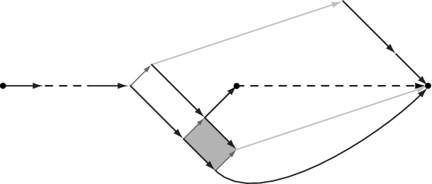
We have to show that is trivial. Suppose instead that is not trivial. Then we may write for some . We have with and . Thus must divide , but holds by -ness of . Therefore, by Lemma 3.11, there exists satisfying , thus , hence . We find with , which contradicts . Therefore, is trivial, which concludes the induction. ∎
A note on the reflection group and the Garside structure
The number of simples in is , while the number of elements in is . For , we have equality between these two expressions, corresponding to the classical type case. For , we have , hence
(For example, there are 35 simples in —see Figure 9—and elements in .) In other words, not all elements of may be represented by simples from . For example, the element
may not be represented by a simple from .
The known classical braid monoids for braid groups of real reflection groups all have equality between number of simples and size of reflection group. In this way the monoid appears not to be strictly classical. However in a number of ways it is seen to be dual, or simply different from, the so-called dual braid monoids, and so deserves a name like post-classical. This is the content of the next subsection.
3.4. How classical is ?
The braid group seems to admit no classical braid monoid, in the sense that its submonoid generated by the generators of [BMR]—providing a minimal generating set—is indeed not finitely presented (see [Co, BC1, BC2]). Recall that the braid monoid (resp. the dual braid monoid ) coincides with the classical braid monoid (resp. the dual braid monoid ) for and with the dual braid monoid for .
In this subsection we look at various properties of the monoid , which mainly deal with enumerative aspects, and consider them in relation to known classical and dual braid monoids for other braid groups. While it cannot be considered as strictly classical, has much in common with the classical braid monoids than with the dual braid monoids, and it could be considered as a post-classical braid monoid. The following three observations allow to legitimate this terminology.
3.4.1. A kind of duality
According to [B2], the duality terminology in the context of Garside monoids for braid groups of finite real reflection groups can be justified by the numerical facts summarized in the following table:33 3 Each of the braid group presentations constructed in [B1] corresponds to a regular degree . The product of the generators raised to the power (which is the order of the image of this product in the reflection group), is always central. See also [B3].
A different kind of duality can be observed between the monoids and :
Thus the monoid may be considered to be a kind of dual of the dual braid monoid . The latter fits into the general framework of dual braid monoids defined in [B2], but it satisfies only some of the numerical properties summarized in the first table above. In a parallel way, could be named simply classical. Here, we could mention that neither nor can be produced by [B1, Theorem 0.1], so in particular, the notion of regular degree is not relevant.
3.4.2. Poincaré polynomial
For a given Garside monoid , the polynomial is defined by where denotes the number of length simples in (see earlier comments preceding Corollary 3.8). In the case of the classical braid monoids associated to finite Coxeter group (for example , , , etc), this polynomial coincides with the Poincaré polynomial of , where is the number of length elements of with respect to a set of simple reflections. In these cases, we have:
where the numbers denote the reflection degrees. The polynomial does not satisfy this general formula, except for the cases or . However the similarity of factorization of the Poincaré polynomial (see below) suggests describing again as a post-classical braid monoid.
3.4.3. Zeta polynomial
For a given Garside monoid , the zeta polynomial can be defined by requiring that be the number of length multichains in the lattice of simples of . Whenever is well-generated (which is the case for ), the zeta polynomial of the dual braid monoid admits a nice factorization:
where are the reflection degrees (see [Ch, R, AR]). On the contrary, the zeta polynomial of the classical braid monoid (when defined) is not known to admit any nice factorization. In this way, has more in common with classical braid monoids than dual braid monoids. For instance, we find:
3.5. Conclusion
While we feel that the new Garside monoid deserves the description post-classical, we do not exclude the possibility that this is the best presentation available, and would like to conclude with a motivating question:
Question 3.12.
Does admit other Garside structures?
4. Acknowledgment
The completion of this work was made possible from a collaboration begun at the GDR Tresses conference in Autrans, 2004 (GDR 2105 CNRS, “Tresses et Topologie de basse dimension” [Aut]).
The first author would also like to thank the European Union for a Marie Curie Postdoctoral Research Award at the time this work was undertaken.
The authors thank Ivan Marin for pointing out to them that, during his thesis work supervised by Daan Krammer, Mark Cummings had discovered the same Garside structure for , even though proofs and motivations are essentially different.
References
- [AR] Ch. Athanasiadis, V. Reiner, Noncrossing partitions for the group , SIAM J. Discrete Math. 18-2 (2004) 397–417 (electronic).
- [Aut] Braids conference in Autrans proceedings (2004).
- [B1] D. Bessis, Zariski theorems and diagrams for braid groups, Invent. math. 145 (2001) 487–507.
- [B2] D. Bessis, The dual braid monoid, Ann. Sci. École Norm. Sup. 36 (2003) 647–683.
- [B3] D. Bessis, Topology of complex reflection arrangements, arXiv:math.GT/0411645.
- [BC1] D. Bessis, R. Corran, Garside structure for the braid group of , arXiv:math.GR/0306186.
- [BC2] D. Bessis, R. Corran, Non-crossing partitions of type , Adv. Math. 202 (2006) 1–49.
- [BDM] D. Bessis, F. Digne & J. Michel, Springer theory in braid groups and the Birman-Ko-Lee monoid, Pacific J. of Math. 205-2 (2002) 287–309.
- [BKL] J. Birman, J., K. H. Ko and S. J Lee, A new approach to the word and conjugacy problems in the braid groups, Adv. Math. 139 (1998) 322–353.
- [Br] E. Brieskorn, Die Fundamentalgruppe des Raumes der regulren Orbits einer endlichen komplexen Spiegelungsgruppe, Invent. Math. 12 (1971) 57–61.
- [BS] E. Brieskorn, K. Saito, Artin-Gruppen und Coxeter-Gruppen, Invent. Math. 17 (1972) 245–271.
- [BMR] M. Broué, G. Malle et R. Rouquier, Complex reflection groups, braid groups, Hecke algebras, J. reine angew. Math. 500 (1998) 127–190.
- [Co] R. Corran, On monoids related to braid groups, Ph. D. dissertation, University of Sydney, May 2000.
- [Ch] F. Chapoton, Enumerative properties of generalized associahedra, Sém. Lothar. Combin. 51 (2004) Art. B51b, 16pp.
- [Cum] M. Cummings, Garside groups and enumeration of partitions, PhD Thesis.
- [Cr] J. Crisp, Injective maps between Artin groups, in “Geometric Group Theory Down Under” ed. J. Cossey et al., de Gruyter Verlag (1999) 119–137.
- [D1] P. Dehornoy, On completeness of word reversing, Discrete Math. 225 (2000) 93–119.
- [D2] P. Dehornoy, Groupes de Garside, Ann. Sci. École Norm. Sup. 35 (2002) 267–306.
- [D3] P. Dehornoy, Thin groups of fractions, Contemp. Math. 296 (2002) 95–128.
- [D4] P. Dehornoy, Complete positive group presentations, J. of Algebra 268 (2003) 156–197.
- [DP] P. Dehornoy, L. Paris Gaussian groups and Garside groups, two generalizations of Artin groups, Proc. of London Math. Soc. 79 (1999) 569–604.
- [Del] P. Deligne, Les immeubles des groupes de tresses généralisés, Invent. Math. 17 (1972) 273–302.
- [Di] F. Digne, Présentations duales des groupes de tresses de type affine , Comment. Math. Helv. 81 (2006) 23–47.
- [G] F. A. Garside, The braid group and other groups, Quart. J. Math. Oxford 20 (1969) 235–254.
- [P] M. Picantin, Explicit presentations for the dual braid monoids, C. R. Acad. Sci. Paris Série I 334 (2002) 843–848.
- [R] V. Reiner, Non-crossing partitions for classical reflection groups, Discrete Math. 177 (1997) 195–222.
- [ST] G.C. Shephard, J.A. Todd, Finite unitary reflection groups, Canad. J. Math. 6 (1954) 274–304.
- [Sh] J.-Y. Shi, Certain imprimitive reflection groups and their generic versions, Trans. Amer. Math. Soc. 354 (2002), no. 5, 2115–2129.
- [Slo] N. J. A. Sloane, The on-line encyclopedia of integer sequences, published electronically at http://www.research.att.com/njas/sequences/.