Scaling factors for ab initio vibrational frequencies:
comparison of uncertainty models for quantified prediction
Abstract
Bayesian Model Calibration is used to revisit the problem
of scaling factor calibration for semi-empirical correction of ab
initio calculations. A particular attention is devoted to uncertainty
evaluation for scaling factors, and to their effect on prediction
of observables involving scaled properties. We argue that linear models
used for calibration of scaling factors are generally not statistically
valid, in the sense that they are not able to fit calibration data
within their uncertainty limits. Uncertainty evaluation and uncertainty
propagation by statistical methods from such invalid models are doomed
to failure. To relieve this problem, a stochastic function is included
in the model to account for model inadequacy, according to the Bayesian
Model Calibration approach. In this framework, we demonstrate that
standard calibration summary statistics, as optimal scaling factor
and root mean square, can be safely used for uncertainty propagation
only when large calibration sets of precise data are used. For small
datasets containing a few dozens of data, a more accurate formula
is provided which involves scaling factor calibration uncertainty.
For measurement uncertainties larger than model inadequacy, the problem
can be reduced to a weighted least squares analysis. For intermediate
cases, no analytical estimators were found, and numerical Bayesian
estimation of parameters has to be used.
Keywords: Bayesian data analysis, Model calibration, Scaling
factor, Vibrational frequency
1Laboratoire de Chimie Physique, CNRS, UMR8000, Orsay, F-91405
2Univ Paris-Sud, Orsay, F-91405
1 Introduction
The final stage in the development of a model, after calibration on an experimental dataset and proper validation, consists in its use for prediction: ”If the experimental dataset is sufficiently broad, there is a reasonable expectation that the results will be accurate to something like the target accuracy”.[1] The estimation of uncertainty for the results of computational chemistry is indeed of paramount importance, notably to their use in multiscale modeling. [2, 3] The concept of Virtual Measurement has been introduced by Irikura[4] to take advantage of the standardized procedures defined by the Guide to the Expression of Uncertainty in Measurement (also known as ”the GUM”),[5] and to apply them in the case of quantum chemistry modeling. Random uncertainties have been shown to be very small, and the major uncertainty factor are biases due to basis-set and/or theory limitations. For quantum chemistry to be predictive, i.e. to be able to predict observables with confidence intervals, one has to correct for these biases, which commonly requires semi-empirical corrections. Uncertainty attached to these corrections have to be considered in the final uncertainty budget, to which they constitute often a major contribution.
Scaling of harmonic vibrational frequencies is an important example of calibration method in computational chemistry, where estimation of a vibrational frequency is obtained by multiplying the corresponding harmonic vibrational frequency , routinely calculated by standard computational chemistry codes, by an empirical scaling factor (Fig. 1)
| (1) |
Optimal scaling factors have been computed for extensive sets of theory/basis-set combinations [6, 7, 8, 9]. In the majority of publications about scaling factors, two summary statistics are provided for each theory/basis-set combination: the optimal scaling factor and the root mean squares. From a reference dataset of experimental and calculated vibrational frequencies the optimal scaling factor obtained by the least-squares procedure is
| (2) |
and the quality of the correction is estimated by the root mean squares (rms) value
| (3) |
To our knowledge, these values are not explicitly used for uncertainty propagation, but the rms provides an estimate of the residual uncertainty resulting from the scaling correction (”something like the target accuracy”[1], or ”a surrogate for uncertainty” according to [10]).

In a recent article (hereafter referred to as Paper I), Irikura et al.[10] treated the problem of uncertainty propagation from scaled frequencies, and, using procedures advocated by the GUM [5], insisted that the scaling factor itself is subject to uncertainty, and proposed that this uncertainty is the major contribution to prediction uncertainty. On the practical side, prediction uncertainty would be proportional to the calculated harmonic frequency; on the factual side, these authors declare that scaling factors for vibrational frequencies are accurate to only two significant figures, whereas all other studies overstate their precision by reporting them with four figures. This approach has been adopted by the National Institute of Standards and Technology (NIST) and put into practice in the Computational Chemistry Comparison and Benchmark DataBase (CCCBDB) [9], section XIII.C.2, where all scaling factors are provided with uncertainties derived according to the procedure of Paper I.
In the present paper, we revisit the problem of scaling factor calibration and we recast it in the Bayesian Model Calibration framework, reputed for providing consistent uncertainty evaluation and propagation [11, 12, 13]. Section 2 presents the methodological elements used for calibration and validation procedures, which are applied to representative vibrational frequency and zero point vibrational energy datasets in Section 3. Bayesian calculations used in this study are fairly standard, but for the sake of completeness and for readers unfamiliar with statistical modeling, details are provided in the Appendix .
2 Methods
2.1 Statistical model for scaling factor calibration
Considering a measured frequency , one can assume that it is related to the true value by
| (4) |
where is a normal random variable centered at zero, with variance , representing the measurement uncertainty in the hypothesis of additive white noise. In the following, we assume that is known beforehand.
Calculated harmonic vibrational frequencies are affected by random errors, related to numerical convergence defined by non-zero thresholds and the choice of starting point in geometry optimization, and to non-zero thresholds in wave-function optimization [4]. It has been shown that the associated uncertainties are negligible when compared to the measurement uncertainties [4]. In the following, one can thus assume that the harmonic vibrational frequencies, being deterministically calculated, have fixed values.
If one makes the hypothesis of a linear relationship between and , the calibration model resulting from this analysis is
| (5) |
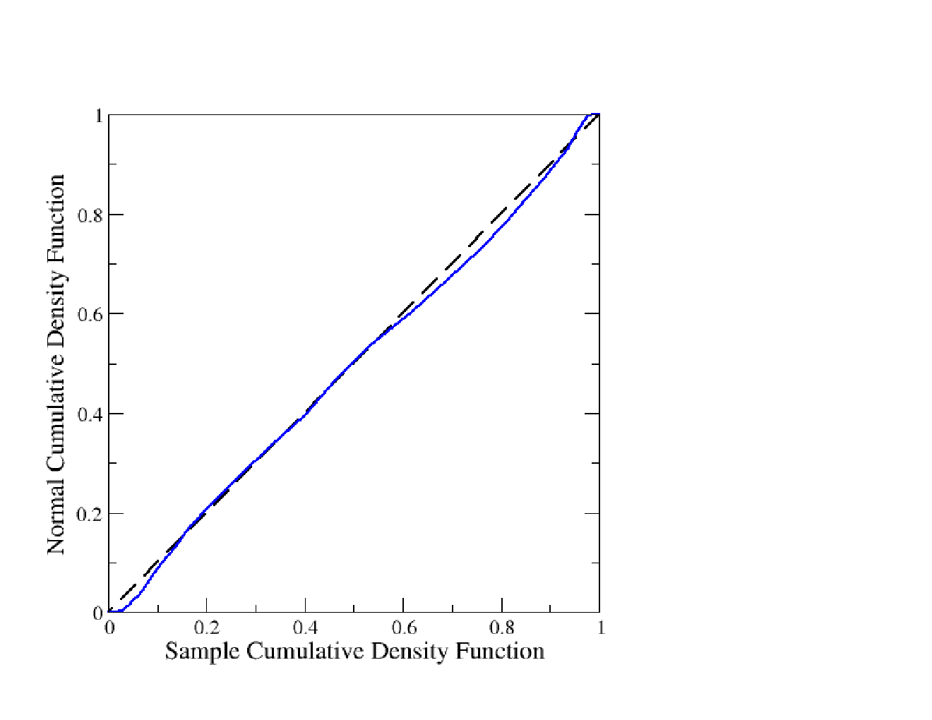
For a single frequency, there is an optimal scaling parameter . As is uncertain, with standard uncertainty , the value of cannot be known exactly and has a standard uncertainty . For a calibration dataset with uniform measurement uncertainty , it can be shown that the optimal value for is still given by Eq. 2, and its standard uncertainty by (c.f. Appendix A.3). Applicability of this formula is subject to one condition: the model (Eq. 5) should be statistically valid. This means that the residuals should have a normal distribution with variance . Normality is not always verified, but most important, the variance condition is typically violated when precise data are used for calibration. The linear model (Eq. 5) is typically unable to reproduce a given set of measured frequencies within their uncertainty range. In such a case, the width of the distribution of residuals is dominated by model misfit, not by measurement uncertainty, and the model is invalid.
An option would be to seach for a better model than the linear scaling, which is beyond the purpose of this study. Instead, we consider here that the misfit is not deterministically predictable. The solution to preserve the linear scaling model in a statistically valid model, is thus to introduce a stochastic variable to represent the discrepancy between model and observations
| (6) |
This equation is similar to the basic statistical model introduced by Kennedy and O’Hagan for Bayesian calibration of model outputs [11]. The discrepancy variable could formally depend on , but we observed that the residuals between model and observations are not notably frequency dependent (Fig. 2), and the same is assumed for which is considered null in average with variance
| (7) |
The calibration equation depends thus on two unknown parameters and .

(A)
 (B)
(B)
2.2 Uncertainty propagation
The calibration model (Eq. 6) being linear with regard to uncertain variables , and , and in the hypothesis of normally distributed uncertainties, we can use the standard uncertainty propagation rules [5] to estimate the value and uncertainty on predicted vibrational frequencies:
| (8) | ||||
| (9) | ||||
| (10) |
The terms due to covariances have been omitted from this equation as the three variables are independent by hypothesis. In order to provide evaluated predictions of vibrational frequencies, we need therefore to estimate , and from the calibration dataset. This is done in the next section, using Bayesian model calibration.
2.3 Bayesian Model Calibration (BMC)
2.3.1 General case
Starting from the statistical calibration model (Eq. 6), one derives the following expression for the posterior probability density function of the parameters, given a set of measured and calculated frequencies (details are reported in Appendix A.1)
| (11) |
Inferences from this pdf have to be done generally by numerical methods [12], as will be applied later to zero point vibrational energies. For vibrational frequencies, we first derive an adapted, simplified, model.
2.3.2 The case of negligible measurement uncertainties
In the commonly met situation where the amplitude of is much larger than the other sources of uncertainty (), we can consider the approximate measurement model
| (12) |
for which the posterior pdf can be simplified to
| (13) |
This expression is amenable to analytical derivation of the estimates for the parameters (see Appendix A.2):
- •
the average value for is identical to the optimal value provided by least-squares analysis ;
- •
the standard uncertainty on , is related to the rms by the formula
; - •
the estimate of is related to according to .
Using these estimates, we can establish an explicit expression for the standard uncertainty of :
| (14) |
Confidence intervals can be defined for prediction purpose, e.g. the 95% confidence interval for , assuming the normality of uncertainty is given by
| (15) |
It can be seen that for large calibration sets of few hundreds of frequencies and , and thus
| (16) |
In such conditions, it is thus possible to derive directly confidence intervals from the the summary calibration statistics and provided by the reference literature.[6, 7, 8]
2.4 The Multiplicative Uncertainty (MU) method
Irikura et al. [10], after a thorough analysis of the uncertainty sources, established that the major contribution to uncertainty propagation would be the uncertainty on the scaling factor . They estimate from the weighted variance of with weights . This weighting scheme is derived in two steps: (1) they propose that the probability density function (pdf) for the scaling factor is a linear combination of pdf’s for individual scaling factors in the reference set; and (2) from the comparison of the expression of the average value derived from this proposition with the least-squares solution Eq.2. This way, they obtain a standard uncertainty
| (17) |
which can be related to by . This uncertainty is different, and generally smaller, than the dispersion of values within the calibration set
| (18) |
The uncertainty on a scaled frequency is then reduced to
| (19) |
hence the name of ”Multiplicative Uncertainty” (MU) used hereafter.
The salient feature of Eq. 19 is that uncertainty should be proportional to the calculated harmonic frequency. But, if one observes correlation plots for reference datasets (e.g. Fig. 1, cm-1), this is not the case. When contrasted with the BMC approach, one understands that the multiplicative approach ”absorbs”, at least partially, model inadequacy in . It is thus implicitly assumed in this approach that the model (Eq. 5) is in a statistical regime, although it is not. These points will be illustrated and discussed in the next section.
3 Applications and discussion
3.1 Vibrational frequencies
We illustrate the BMC and MU approaches on the HF/6-31G* combination of theory/basis-set. The reference dataset, plotted in Fig. 1, has been downloaded from the NIST/CCCBDB in July 2008.[9]
3.1.1 Calibration
Using the BMC model and estimators on the reference set, we obtain , and cm-1 (Table 1), which is consistent with the value of the rms obtained by Merrick et al. [8] for the same theory/basis-set combination. For this dataset, the CCCBDB proposes . We cross-checked this value using Eq. 17 (Table 1). The standard uncertainty on evaluated by both methods differ thus by a factor 50, which is expected to have noticeable effect on prediction uncertainty. In order to visualize this effect, we plotted the 95 percent confidence intervals in both cases (Fig. 3). It is immediately visible that the the MU approach has a tendency to underestimate uncertainty at low frequencies and to overestimate it at high frequencies. In comparison, the BMC approach is more balanced.
| Summary stat. | MU | BMC | ||||||||
| (cm-1) | %CI95 | (cm-1) | %CI95 | |||||||
| All frequencies (2738) | ||||||||||
| Full set | 0.8984 | 0.069 | 45.3 | 0.024 | - | 0.0005 | 45.3 | - | ||
| Calibration set | 0.8986 | 45.3 | 0.024 | - | 0.0007 | 45.3 | - | |||
| Validation set | - | - | - | - | 83.0 | - | - | 94.6 | ||
| Frequencies between 3180 and 3500 cm-1 (479) | ||||||||||
| Full set | 0.9050 | 0.0087 | 28.7 | 0.0087 | - | 0.0004 | 28.8 | - | ||
| Calibration set | 0.9052 | 23.3 | 0.0071 | - | 0.0005 | 23.4 | - | |||
| Validation set | - | - | - | - | 95.0 | - | - | 95.4 | ||

3.1.2 Validation
In order to comfort the observations of the previous section (3.1.1), we split the calibration dataset in two subsets by using the odd indexes for calibration, and the even ones for validation (the frequencies being ordered per molecule, this provides a quasi-random selection with regard to frequency value). In this case, one gets slightly different values of the parameters, as reported in Table 1. Using these values, we generate 95% confidence intervals and calculate the frequency of inclusion of the experimental values of the validation subset within these intervals (Fig. 3). For a consistent estimator, one should find a frequency close to 95%. BMC succeeds for 94.7%, whereas the MU model succeeds for only 83% of the frequencies in the validation set (Table 1). Considering the size of tha samples, the difference is significative, and the consistency of the multiplicative uncertainty approach in this context can be questioned.
3.1.3 Test on a restricted frequency scale
As stated in Paper I, ”to apply the fractional bias correction, it is important to select a class of frequencies similar to the ones to be estimated”. For instance, if one selects in the reference set only those frequencies between 3180 and 3500 cm-1, one gets a much more uniform picture than with the full reference set. The calibration procedure was done with this limited set of 479 frequencies, providing (Table 1). In this case, we note that the uncertainty factor for is practically identical to the standard deviation calculated from the sample (0.00869 vs. 0.00871): . Due to the restricted frequency range, one has indeed (cf. Eqs 17 and 18).
The restricted set has been split in two using index parity, as before. The scaling factor obtained by MU from the calibration subset is now , and 95.0% of the validation frequencies fall within the 95% confidence interval. This result is now identical to the one obtained with BMC (Table 1), the confidence intervals obtained by both methods being indistinguishable.
It appears thus that in restrictive conditions, the MU method can be valid for reference sets where the individual scaling factors are uniformly distributed with regard to the harmonic frequencies. In such case however, the uncertainty is reduced to a conventional unweighted standard deviation.
3.1.4 Uncertainty propagation
The relative importance of both factors and ( in this example) in Eq. 10 can be evaluated on the example of a calculated harmonic frequency in the higher range cm-1 (Table 2). In this case, the uncertainty on the scaling factor contributes only to one thousandth of the total prediction variance.
For any practical purpose, the uncertainty on the scaling factor of vibrational frequencies can therefore be neglected. The uncertainty on is also much too small to be relevant for confidence intervals calculation. One can thus safely apply the uncertainty propagation formula (Eq. 16), using the rms provided by most reference articles dealing with scaling factors calibration [6, 7, 8].
| (HF/6-31G*) | ||||
|---|---|---|---|---|
| Freq. | 3000 | 2.25 | 2052.09 | 269545 cm-1 |
| ZPVE | 100 kJ mol-1 | 0.029 | 0.194 | 98.120.47 kJ mol-1 |
3.2 Zero Point Vibrational Energies
We consider ZPVE as a an additional test because the reference datasets are considerably smaller than for the vibrational frequencies (e.g. 39 molecules in the Z1 set of Merrick et al. [8]), which is expected to enhance the role of the uncertainty on the scaling factor. In the absence of a systematic review of measurement errors for ZPVE of polyatomic molecules, we consider in the following that they can be neglected. The uncertainties reported by Irikura [14] for diatomic molecules are indeed very small (on the order of 0.01 cm-1), but transposition to larger molecules is not straightforward.
Using our measurement model and estimators on the reference set, one gets and kJ mol-1 (Table 3), which is consistent with the rms obtained by Merrick et al. [8] for the HF/6-31G* theory/basis-set combination. Relative uncertainties on these parameters have been increased by one order of magnitude, compared with the vibrational frequencies case. The validation exercise shows once more that the Multiplicative Uncertainty model fails to provide correct confidence intervals, with a score of only 0.63 for CI95.
In such a case of small reference dataset, it is interesting to check if the approximate formula (Eq. 16) for uncertainty propagation which was validated for large sets of vibrational frequencies begins to break down, i.e. the contribution of the multiplicative term involving stays negligible or not, for the larger ZPVE values. For instance, if one considers a calculated ZPVE of 100 kJ mol-1, one has kJ mol-1, to be compared to kJ mol-1. It is to be noted also that the uncertainty on might contribute at the same level, kJ mol-1. Taking all uncertainty sources into account trough Eq. 51 by Monte Carlo Uncertainty Propagation, one gets kJ mol-1. Apparently, the fluctuations of do not have an effect and only the uncertainty on the scaling factor has a noticeable effect, albeit quite small.
In the same conditions, for the combination B3LYP/6-31G*, one gets kJ mol-1 and kJ mol-1, to be compared with an exact value of kJ mol-1 (Table 3). There is globally only a 10% increase compared to the rms . In this range of ZPVEs, still provides a good approximation of the uncertainty factor (Table 2). However, the amplitude of the discrepancy between and will probably increase with the size of the molecule. In consequence, for uncertainty propagation with ZPVEs, notably for large molecules, it would be safer to use the full UP formula (Eq. 14), involving the multiplicative uncertainty factor. Compilations of scaling factors should thus report the easily calculated value of , in addition to the rms .
| Summary stat. | MU | BMC | ||||||||
| (kJ mol-1) | %CI95 | (kJ mol-1) | %CI95 | |||||||
| HF/6-31G* | ||||||||||
| Full set | 0.9135 | 0.0607 | 0.71 | 0.0161 | - | 0.0027 | 0.730.09 | - | ||
| Calibration set | 0.9078 | 0.77 | 0.0214 | 0.0052 | 0.830.14 | |||||
| Validation set | 0.63 | 0.95 | ||||||||
| B3LYP/6-31G* | ||||||||||
| Full set | 0.9812 | 0.0375 | 0.42 | 0.0103 | - | 0.0017 | 0.440.05 | - | ||
| Calibration set | 0.9825 | 0.45 | 0.0134 | 0.0032 | 0.480.08 | |||||
| Validation set | 0.68 | 1.00 | ||||||||
3.2.1 Non-negligible experimental uncertainties
When the measurement uncertainty becomes comparable to the rms, model discrepancy should be vanishing, and confidence intervals for prediction should include the measurement uncertainty, i.e. . In the absence of an exhaustive compilation of experimental uncertainties on measured ZPVE, we performed simulations assuming a uniform uncertainty distribution over the full dataset. In order to test the sensitivity of the model parameters to this uncertainty, we repeated the estimations of previous section, using Eq. 27, for different values of between 0.1 and 1.0 kJ mol-1. The results are reported in Fig. 4.
As expected from the properties of the posterior pdf, the average/optimal value of the scaling factor is insensitive to the amplitude of . Moreover, we observe only a slight increase of from 0.002 to 0.004. A transition from a constant , defined by the limit, to a linear increase consistent with the weighted least squares limit (Eq. 50) is observed around , where both limits intersect. A closer look shows that the transition occurs indeed at values of slightly smaller than , in a region ( where displays a minimum.
The evolution of is more dramatic: it displays a sharp decrease and falls down to zero as soon as the measurement uncertainty reaches and overpasses the value of the rms . For values of below , obeys to the law (represented as a dashed line in Fig. 4), but the calculated decrease becomes much faster in the transition zone. The uncertainty on increases notably in the transition region observed for .
In the limit of large experimental uncertainties, the uncertainty propagation formula can be written as
| (20) | ||||
| (21) |
In this region of large measurement uncertainty, the inadequacy variable becomes useless, as the calibration with the scaling factor alone enters a statistical regime.

4 Conclusion
A reanalysis of scaling factors calibration in the aim of providing quantified predictions shows that for large validation sets of accurate data, as used for vibrational frequencies, faithful prediction uncertainties can be derived from the standardly reported optimal scaling factor and rms. For much smaller datasets of a few dozens of data, as in the case of ZPVEs, uncertainty on the scaling factor should also be reported. The following limit formulas have been validated and are proposed for uncertainty propagation from a given calculated harmonic frequency :
- •
large calibration sets of precise data (): ;
- •
small calibration sets of precise data (): ;
- •
sets of data with large uniform uncertainty (): .
A general estimation framework, based on Bayesian Model Calibration, has been defined for those cases where the limit conditions defined above are not met.
The Multiplicative Uncertainty method proposed by Irikura et al. [10] () has been shown to be inconsistent when large frequency ranges are considered. It could not be recovered by the Bayesian approach, except when the dataset spans a restricted frequency range, in which case it is reduced to a trivial, unweighted, standard deviation. The use of the scaling factor uncertainties as reported presently (November 2008) in the CCCBDB[9] cannot therefore be recommended.
I would like to stress out that the validity of the formulas for uncertainty propagation depends to some extent on the normality of the residuals of the linear regression. Inspection of histograms of residuals (see e.g. Fig.1 in Ref. [7]) shows that this is not always the case. The customary approach to choose an optimal theory/basis-set combination is to assess their performance by the rms alone, maybe weighted by computational cost considerations [6, 7, 8]. One could also consider a ”normality criterion” in order to reject theory/basis-set combinations providing non-normal residuals and from which the summary statistics cannot be used faithfully for uncertainty propagation. Analysis of restricted ranges of data as presently done by some authors for vibrations[8] is one way to improve the normality of residuals.
Semi-empirical correction of ab-initio results by scaling is presently very common and efficient for many observables. It certainly would be a large step towards the general applicability of uncertainty propagation, if statistically pertinent estimators were systematically reported in the literature devoted to the calibration of these correction models.
Acknowledgments
I would like to thank Prof. Leo Radom for providing me with the Z1 ZPVE dataset. B. Lévy is warmly acknowledged for helpful discussions.
Appendix A Appendix
A.1 Bayesian analysis of scaling factor calibration model
We consider the measurement model
| (22) |
where is the measurement uncertainty of , and is a discrepancy function between the linear model and the observations. This model has two unknown parameters, and , to be estimated on a calibration dataset consisting of calculated harmonic frequencies , and their corresponding observed frequencies .
In the Bayesian data analysis framework,[15, 12] all information about parameters can be obtained from the joint posterior pdf . In order to simplify the notations, we will omit in the following the list indices when they are not necessary.This pdf is obtained through Bayes theorem
| (23) |
where is the likelihood function and is the prior pdf.
As the difference between observation and corrected frequency has a normal distribution
| (24) |
the likelihood function for a single observed frequency is
| (25) |
Considering that all frequencies are measured independently (with uncorrelated uncertainty) the joint likelihood is the product of the individual ones, i.e.
| (26) |
As there is a priori no correlation between and , we use a factorized prior pdf . In the absence of a priori quantified information on , a uniform pdf is used. For we have to consider a positivity constraint, and we use a Jeffrey’s prior, . The posterior pdf is finally defined up to a proportionality factor which is irrelevant for the following developments
| (27) |
A.2 Case of negligible measurement uncertainties
For the analysis of vibrational frequencies, it is generally considered that experimental uncertainties are negligible (). The general expression for the posterior pdf (Eq. 27) can be simplified accordingly to
| (28) |
Using the identity
| (29) |
it can be written in a convenient factorized form
| (30) |
from which we can derive analytical estimates for the parameters and their uncertainties.
A.2.1 Estimation of
The marginal density for is obtained by integration over
| (35) |
Posing and , we can directly use the properties of the Student’s distribution
| (36) |
to derive
| (37) | ||||
| (38) |
A.2.2 Estimation of
The marginal density for the standard uncertainty of the stochastic variable is
| (39) | |||||
| (40) | |||||
| (41) |
Using the formula
| (42) |
one obtains readily the following estimates
| (43) | ||||
| (44) | ||||
| (45) | ||||
| (46) |
A.3 Case of very large measurement uncertainties
When model discrepancy is negligible compared to measurement uncertainties, i.e. when the standard linear model is in a statistical regime, one recovers standard statistical analysis, the Bayesian analog to weighted least squares. The posterior pdf for is then
| (47) |
from which one obtains
| (48) | ||||
| (49) |
For uniform experimental uncertainty over the dataset, the scaling factor uncertainty varies linearly with
| (50) |
A.4 Uncertainty propagation
In the Bayesian framework, the posterior pdf can be used to estimate the uncertainty of predicted frequencies
| (51) |
where
| (52) |
results from the stochastic model (Eq. 12). This integral has generally to be evaluated numerically.
References
- [1] John A. Pople. Nobel lecture: Quantum chemical models. Rev. Mod. Phys., 71(5):1267–1274, 1999.
- [2] Carmen Pancerella, James D. Myers, Thomas C. Allison, Kaizar Amin, Sandra Bittner, Brett Didier, Michael Frenklach, Jr. William H. Green, Yen-Ling Ho, John Hewson, Wendy Koegler, Carina Lansing, David Leahy, Michael Lee, Renata McCoy, Michael Minkoff, Sandeep Nijsure, Gregor von Laszewski, David Montoya, Reinhardt Pinzon, William Pitz, Larry Rahn, Branko Ruscic, Karen Schuchardt, Eric Stephan, Al Wagner, Baoshan Wang, Theresa Windus, Lili Xu, and Christine Yang. Metadata in the Collaboratory for Multi-Scale Chemical Science. In 2003 Dublin Core Conference: Supporting Communities of Discourse and Practice-Metadata Research and Applications, Seatle, WA, 28 September – 2 October 2003.
- [3] M. Frenklach. Transforming data into knowledge. Process Informatics for combustion chemistry. Proceedings of the Combustion Institute, 31:125–140, 2007.
- [4] K.K. Irikura, R.D. Johnson III, and R.N. Kacker. Uncertainty associated with virtual measurements from computational quantum chemistry models. Metrologia, 41:369–375, 2004.
- [5] BIPM, IEC, IFCC, ISO, IUPAC, IUPAP, and OIML. Guide to the expression of uncertainty in measurement (GUM). Technical Report ISBN 92-67-10188-9, International Organization for Standardization, Geneva, 1995. Corrected and reprinted.
- [6] A.P. Scott and L. Radom. Harmonic Vibrational Frequencies: An Evaluation of Hartree-Fock, Möller-Plesset, Quadratic Configuration Interaction, Density Functional Theory, and Semiempirical Scale Factors. J. Phys. Chem., 100(41):16502–16513, 1996.
- [7] Ming Wah Wong. Vibrational frequency prediction using density functional theory. Chemical Physics Letters, 256(4-5):391–399, 1996.
- [8] J.P. Merrick, D. Moran, and L. Radom. An evaluation of harmonic vibrational frequency scale factors. J. Phys. Chem. A, 111(45):11683–11700, 2007.
- [9] R.D. Johnson III. NIST Computational Chemistry Comparison and Benchmark Database, Release 14; NIST Standard Reference Database Number 101, September 2006. http://cccbdb.nist.gov/.
- [10] K.K. Irikura, R.D. Johnson, and R.N. Kacker. Uncertainties in scaling factors for ab initio vibrational frequencies. J. Phys. Chem. A, 109(37):8430–8437, 2005.
- [11] Marc C. Kennedy and Anthony O’Hagan. Bayesian calibration of computer models. Journal of the Royal Statistical Society: Series B (Statistical Methodology), 63(3):425–464, 2001.
- [12] P. Gregory. Bayesian Logical Data Analysis for the Physical Sciences. Cambridge University Press, 2005.
- [13] BIPM, IEC, IFCC, ISO, IUPAC, IUPAP, and OIML. Evaluation of measurement data - Supplement 1 to the GUM: propagation of distributions using a Monte Carlo method. Technical report, BIPM, September 2006. Final draft.
- [14] Karl K. Irikura. Experimental vibrational zero-point energies: Diatomic molecules. J. Phys. Chem. Ref. Data, 36(2):389–397, 2007.
- [15] D.S. Sivia. Data Analysis: A Bayesian Tutorial. Clarendon (Oxford Univ. Press), Oxford, 1996.
- [16] M. Evans, N. Hastings, and B. Peacock. Statistical Distributions. Wiley-Interscience, 3rd edition, 2000.