Revising the predictions of inflation for the cosmic microwave background anisotropies

A sufficiently long period of accelerated expansion in the very early universe is able to solve the questions raised by the standard big bang cosmology [1]. The hot big bang cosmology is an extremely successful theory. It explains the existence of the cosmic microwave background (CMB) and its thermal nature, the observed expansion of the universe, the abundance of light elements and the astrophysical fits for the age of the universe. However, it leaves without answer why our universe appears so homogeneous and nearly flat at large scales. Inflation offers a natural answer to these questions and, at the same time, provides a predictive mechanism to account for the small observed inhomogeneities [2] responsible for the structure formation in the universe and the anisotropies present in the cosmic microwave background (CMB), as first detected by the COBE satellite and further analyzed by the Wilkinson Microwave Anisotropy Probe (WMAP) satellite [3]. Inflation predicts production of primordial density perturbations and relic gravitational waves as amplifications of vacuum fluctuations together with a quantum-to-classical transition at the scale of Hubble sphere crossing. Primordial perturbations leave an imprint in the CMB anisotropies, which are, therefore, of major importance for understanding our universe and its origin. The potential-energy density of a scalar (inflaton) field is assumed to cause the inflationary expansion, and the amplification of its quantum fluctuations and those of the metric are inevitable consequences in an expanding universe [4]. The metric fluctuations provide the initial conditions for the acoustic oscillations of the plasma at the onset of the subsequent radiation-dominated epoch. The detection of the effects of primordial gravitational waves in future high-precision measurements of the CMB anisotropies, as for instance in the PLANCK satellite mission [5], will serve as a highly non-trivial test for inflation. Therefore, it is particularly important to scrutinize, from all points of view, the standard predictions of inflation (as summarized for instance, in [6]) to be tested empirically. This is the aim of this paper. We point out that if quantum field renormalization is taken into account, as in the experimentally tested Casimir effect, the quantitative predictions of inflation change significantly, and may be tested in forthcoming CMB measurements.

The scalar perturbations, which constitute the “seeds” for structure formation, are characterized by the power spectrum

where $\phi$ represents the inflaton scalar field, which dominates the energy density during inflation. Here $H$ stands for the Hubble rate $H\equiv\dot{a}/a$, where $a(t)$ is the expansion factor and dot means derivative with respect to the comoving time. The above expression is evaluated at the Hubble radius crossing time $t_{k}$ (usually called “horizon crossing” time), where $k/a(t_{k})=H$. In the typical slow-roll inflationary scenario the homogeneous part of the inflaton field $\phi_{0}(t)$ rolls slowly down its potential $V(\phi)$ towards a minimum. Both $\phi$ and $H\equiv\sqrt{\frac{8\pi G}{3}V(\phi_{0})}$ are changing very gradually and this change is parameterized by the slow-roll parameters $\epsilon,\eta$, where $\epsilon\equiv-\dot{H}/H^{2}$, and $\eta-\epsilon\equiv\ddot{\phi}/(H\dot{\phi})$. These parameters can be related to the derivatives of the inflaton potential $\epsilon=(M_{P}^{2}/2)(V^{\prime}/V)^{2},\eta=M_{P}^{2}(V^{\prime\prime}/V)$, where $M_{P}=1/\sqrt{8\pi G}$ is the reduced Planck mass in natural units $\hbar=1=c$. In the slow-roll approximation, $\epsilon\ll 1$ and $|\eta|\ll 1$, the scalar power spectrum turns out to be

In addition, the power spectrum of tensor fluctuations is given by

and the tensor-to-scalar ratio is then $r=P_{t}/P_{\cal R}=16\epsilon$. The power spectra are not exactly scale invariant, they can vary with $k$ and this dependence is parameterized by the scalar and tensorial spectral indices $n_{s}-1\equiv d\ln P_{\cal R}/d\ln k,\ n_{t}\equiv d\ln P_{t}/d\ln k$. Since these indices are related to the slow-roll parameters $n_{s}-1=-6\epsilon+2\eta\ ,n_{t}=-2\epsilon$, one generates immediately the consistency relation $r=-8n_{t}$, which should be verified by any single-field slow-roll inflationary model, irrespective of the particular form of the potential.

In this paper we shall reexamine, on the basis of general principles of quantum field theory in an expanding background [7, 8], the fundamental expressions (2-3) for the scalar and tensorial power spectrum. In doing this we shall also be led to modify the expressions for the spectral indices in terms of the slow-roll parameters and, therefore, to generate a new consistency relation. We will have all the necessary ingredients to reexamine the observational predictions of inflationary models and here we shall do that for some of the most significant models.

The second factor in the fundamental relation (1) has its origin in the quantum fluctuation of the scalar inflaton field $\phi$. The first-order perturbation $\delta\phi$, where $\phi=\phi_{0}(t)+\delta\phi(x)$, obeys the wave equation

where $a(t)$ is the expansion factor of the unperturbed homogeneous and spatially flat metric $ds^{2}=-dt^{2}+a^{2}(t)d\vec{x}^{2}$. The effective mass term, which is necessarily small in the slow-roll approximation, is given by the second derivative of the potential: $m^{2}=V^{\prime\prime}(\phi_{0})$. Moreover, the fundamental relation (3) has also the same quantum origin. The two independent polarizations of tensorial modes can be described by a couple of scalar fields $h_{+,\times}$ obeying the above wave equation with zero mass. The relation between $h$ (we omit the subindex $+$ or $\times$) and $\delta\phi$ is given by $\delta\phi\equiv h/\sqrt{16\pi G}$.

Let us focus first on these tensorial perturbations. The form of the modes is then $h_{\vec{k}}(t,\vec{x})=(-16\pi G\tau\pi/4(2\pi)^{3}a^{2})^{1/2}H^{(1)}_{\nu}(-k\tau)e^{i\vec{k}\vec{x}}$. The index of the Bessel function is $\nu=\sqrt{9/4+3\epsilon}$ and the so-called conformal time, $\tau\equiv\int dt/a(t)$, is given by $\tau=-(1+\epsilon)/aH$. Notice that, at early times, the amplitude of oscillations depends on $k$ in a way similar to that of a massless field in Minkowski space. As time evolves, the comoving wavelength reaches the Hubble horizon length at $t_{k}$. A few Hubble times after horizon exit the amplitude freezes completely and, for all subsequent times t, one has the constant value $|h_{\vec{k}}|^{2}=\frac{GH^{2}(t_{k})}{\pi^{2}k^{3}}$. Because of the loss of phase information, the modes of the perturbations soon take on classical properties [9]. The freezing amplitude is usually codified through the quantity $\Delta_{h}^{2}(k,t)$, defined in general by $\Delta_{h}^{2}=4\pi k^{3}|h_{\vec{k}}(t)|^{2}$, and evaluated at the horizon crossing $t_{k}$ (or a few Hubble times after it). Taking into account the two polarizations, one finally obtains a nearly “scale free” tensorial power spectrum (3). In a similar way one obtains the scalar power spectrum (2).

At this stage it is important to remark that the above definition of the power spectrum is such that the quantum fluctuations of the perturbations in position space satisfy the relation

This quantity represents the variance of the Gaussian probability distribution associated to $h(\vec{x},t)$. However, in the form given by (5), it is divergent. It might be argued, as is common when dealing with random fields, that this divergence can be eliminated by smoothing out the field on a certain scale $R$ to remove the Fourier modes with $k^{-1}<R$. It can also be argued that the value of $\langle h^{2}\rangle$ is unimportant and regard the (finite) two-point function $\langle h(x_{1})h(x_{2})\rangle$, uniquely defined by $\Delta^{2}_{h}(k)$, as the basic object. However, it is our view to regard the variance as the basic physical object, which defines the amplitude of fluctuations in position space, and treat $h(\vec{x},t)$ as a quantum entity. Therefore, if one regards $h(\vec{x},t)$ as a quantum field, and $\langle h^{2}(\vec{x},t)\rangle$ its two-point function at coincident points, the divergences must be handled in a different way. Taking into account the large $k$ asymptotic form of the modes one can estimate the form of the integral at an arbitrary time

The first term produces a quadratic divergence, which is the typical singularity of a quantum field in Minkowski space. The second term produces a logarithmic divergence, which is typical of a massless field in an expanding universe. For a quantum mechanical system, with a finite number of degrees of freedom, such a divergent behavior would not arise and one need not worry about the definition of the physical power spectrum. However, a quantum field is neither a random field nor a quantum mechanical system with a finite number of degrees of freedom. The existence of divergences tells us that the nature of a quantum field is more involved. If we wish to have a finite expression for $\langle h^{2}(\vec{x},t)\rangle$ one should subtract the divergences in a consistent way. In technical words, one should renormalize the quantum field. Since the physically relevant quantity (power spectrum) is expressed in momentum space, the natural renormalization scheme to apply is the so-called adiabatic subtraction [10], as it renormalizes the theory in momentum space. Adiabatic renormalization [11, 7, 8] removes the divergences present in the formal expression (5) by subtracting $(16\pi Gk^{3}/4\pi^{2}a^{3})[1/w+\dot{a}^{2}/2a^{2}w^{3}+\ddot{a}/2aw^{3}]$ mode by mode in the integral (5), where $w$ is the frequency of the modes. The subtraction of the first term $(16\pi Gk^{3}/4\pi^{2}a^{3}w)$ to cancel the typical flat space vacuum fluctuations was already considered in [12]. However, the additional terms, proportional to $\dot{a}^{2}$ and $\ddot{a}$ are necessary to properly perform the renormalization in an expanding universe. Subtracting consistently the divergent terms one obtains the finite expression

For the idealized case of a strictly constant $H$ the subtraction exactly cancels out the vacuum amplitude [10] since $H^{(1)}_{3/2}(x)=i\exp(ix)\sqrt{2/\pi x}(-1+i/x)$. From this it follows that in pure de Sitter inflation there is no production of gravitational waves. One would thus expect that the tensorial power spectrum were proportional to the $\epsilon$ slow-roll parameter, which parameterizes the slow change in $H(t)$. The fluctuations still acquire classical properties through decoherence in a time of order $H^{-1}$ after their wavelengths become larger than the Hubble radius during inflation [9]. Therefore, it is natural to evaluate the power spectrum (with the corresponding adiabatic counterterms) a few Hubble times after the time $t_{k}$. Since the results will not be far different from those at $t_{k}$, we use that time to characterize the results. We comment further on this point after (14). Evaluation of the above integral at the time $t_{k}$ leads to the redefinition

which turns out to be proportional to $\epsilon$, $\Delta^{2}_{h}(k)=\alpha 16\pi G(H(t_{k})/2\pi)^{2}\epsilon(t_{k})+O(\epsilon^{2})$, where $\alpha$ is a numerical coefficient of order unity, $\alpha\approx 0.904$. Taking into account the usual conventions, we get, at leading order in $\epsilon$,

One can proceed in the same way to reevaluate the scalar power spectrum. However, to be precise in the calculation, one must keep the mass term in (4) and also take into account the slow decay of the Hubble rate $H$, as above. The latter is controlled by the slow-roll parameter $\epsilon$, while the former is captured by the slowly changing parameter $\eta\equiv M_{P}^{2}(V^{\prime\prime}/V)$, which gives $m^{2}=3\eta H^{2}$. The form of the scalar modes is the same as that for the tensorial ones, up to the fact that the coefficient $\sqrt{16\pi G}$ is now absent and the Bessel index is now $\nu^{2}=9/4+3\epsilon-3\eta$. The adiabatic subtracting terms are then those already present for a massless field, with $w(t)=\sqrt{k^{2}/a^{2}+m^{2}}$, together with new terms proportional to the mass $(k^{3}/4\pi^{2}a^{3})[m^{2}\dot{a}^{2}/2a^{2}w^{5}+m^{2}\ddot{a}/4aw^{5}-5m^{4}\dot{a}^{2}/8a^{2}w^{7}]$. Therefore, after renormalization, the final result for the scalar power spectrum is

where $\beta\approx 0.448$ is another numerical coefficient. In the case of eternal de Sitter expansion, one recovers the previous results of [10, 13].

The above expression, together with (9) for the tensorial power spectrum, constitute our main results and lead to a change in the testable predictions of inflation. To see this we have to consider the scalar and tensorial spectral indices. The standard expression for them, in terms of the slow-roll parameters, is $n_{s}-1=-6\epsilon+2\eta\ ,n_{t}=-2\epsilon$. However, if we invoke renormalization we get

where $n^{\prime}_{t}$ is the running of the tensorial index $n^{\prime}_{t}\equiv d{n_{t}}/d\ln{k}$. Note that $n^{\prime}_{t}$ can be expressed in terms of the slow-roll parameters as $n^{\prime}_{t}=8\epsilon(\epsilon-\eta)+2\xi$, where $\xi$ is defined by $\xi\equiv M_{P}^{4}(V^{\prime}V^{\prime\prime\prime}/V^{2})$. The above formulae provide, implicitly, algebraic relations between physical observables. The most important one is the relation between the tensor-to-scalar ratio $r\equiv P_{t}/P_{\cal{R}}$ with the spectral and running indices: $r=r(n_{t},n_{s},n^{\prime}_{t})$. In the simplest case of $n^{\prime}_{t}=0$, and taking the approximation $\alpha\approx 2\beta$, the new consistency condition becomes

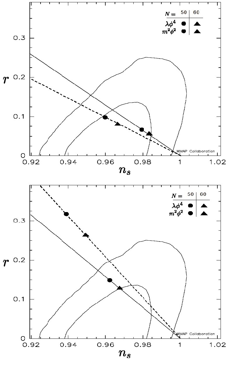
This relation could be potentially checked, and compared with the standard one $r=-8n_{t}$, in near future high-precision anisotropy measurements of the CMB. However, we can already contrast, partially, our predictions with the standard ones on the basis of the five year WMAP results by performing a model by model analysis. As a representative example we shall reexamine the monomial chaotic potential $V(\phi)=\lambda M_{P}^{(4-p)}\phi^{p}$ and compare with standard theoretical and experimental results [3]. It is not difficult to obtain that

where $N\equiv\ln{a_{end}/a_{WMAP}}$ is the number of $e$-folds of inflation between the end of inflation and the epoch when the wavelength of fluctuations that WMAP detects left the horizon. If the adiabatic counterterms were evaluated some $e$-folds $n$ after $t_{k}$ but still well before the end of inflation ($n\epsilon\ll 1$), then the value of $\alpha$ in the tensorial power spectrum would change to $\alpha\approx 2n$. A similar calculation for the scalar power spectrum should also be carried out. This computation should deal with the gauge-invariant quantity ${\cal{R}}_{k}$, which is conserved outside the Hubble sphere and satisfies the same equation as $h_{\vec{k}}$, up to the replacement $a\to a\dot{\phi}_{0}/H$. The result is then $\alpha\approx 6n$, $3\beta\approx-2n$. One then finds that the spectral index $n_{s}$ in (14) is unchanged, and the ratio $r$ becomes $r=4p^{2}/(p+2)N$, which is not sensitive to the value of $n$. If the counterterms are evaluated far beyond the end of inflation, one recovers the standard predictions $r=4p/N$ and $1-n_{s}=(p+2)/2N$. However, since primordial fluctuations acquire classical properties through decoherence when their wavelengths become larger than the Hubble radius [9], we find it natural to evaluate the spectra at a time close to $t_{k}$, which implies significant deviations from the standard prediction (see (14)). Note that, with the present understanding of the nonlinear aspects of quantum gravity, it is difficult to reach a definitive conclusion regarding this question, so the fact that there are observable differences offers a deep way to experimentally probe this question. In fact, if we compare the results at $t_{k}$ with the WMAP 5-year data for the representative values $p=2$ and $p=4$ (Figure 1) we find that both models are compatible with the experimental data for the reasonable range of $N$ between $50$ and $60$ (Figure 1 top). This is in sharp contrast with the prediction of the standard approach (Figure 1 bottom) where the monomial potential with $p=4$ is excluded convincingly. With the new predictions both models are compatible with WMAP data for all the values of $N$ between $50$ and $60$. This is also true even if the counterterms are evaluated $n$ $e$-folds after $t_{k}$, with $n\epsilon\ll 1$. The alternative predictions presented here may soon come within the range of measurement of high-precision CMB experiments, as expected in the PLANCK satellite mission. Acknowledgements This work has been supported by grant FIS2008-06078-C03-02. L.P. has been partly supported by NSF grants PHY-0071044 and PHY-0503366 and by a UWM RGI grant. I.A. and G.O. thank MICINN for a FPU grant and a JdC contract, respectively.

References

- [1] Guth A., Phys. Rev. D23, 347 (1981). Starobinsky A.A., Phys. Lett. B91, 99 (1980). Linde, A.D., Phys. Lett. B108, 389 (1982); Phys. Lett. B129, 177 (1983). Albrecht A. and Steinhardt P. J., Phys. Rev. Lett. 48,1220 (1982). Sato, K., Mon. Not. Roy. Astron. Soc. 195, 467 (1981).
- [2] Mukhanov V.F. and Chibisov G.V., JETP Letters 33, 532(1981). Hawking, S. W., Phys. Lett. B115, 295 (1982). Guth A. and Pi, S.-Y., Phys. Rev. Lett. 49, 1110 (1982). Starobinsky, A. A., Phys. Lett. B117, 175 (1982). Bardeen, J.M., Steinhardt, P.J. and Turner, M.S., Phys. Rev.D28, 679 (1983).
- [3] Komatsu, E. et al, arXiv:0803.0547.
- [4] Parker L., Phys.Rev.Lett. 21 562 (1968); Phys. Rev. 183, 1057(1969).
- [5] Efstathiou G., Lawrence C. and Tauber J., ESA-SCI(2005)1
- [6] Liddle A. R., and Lyth D.H., Cosmological inflation and large-scale structure, CUP (2000). Dodelson S., Modern Cosmology, Academic Press, (2003). Weinberg S., Cosmology, OUP (2008).
- [7] Parker L. and Toms D.J., Quantum field theory in curved spacetime: quantized fields and gravity, CUP (2009)
- [8] Birrel N.D. and Davies P.C.W., Quantum fields in curved space, Cambridge University Press, (1982).
- [9] Kiefer C., Lohmar I., Polarski D., Starobinsky A. A., Class. Quant. Grav. 24 1699 (2007)
- [10] Parker L., hep-th/0702216
- [11] Parker L. and Fulling S.A., Phys. Rev. D 9 341 (1974).
- [12] Linde A., Particle physics and inflationary cosmology, CRC Press (1990). Padmanabhan T., Structure formation in the universe, CUP (1993).
- [13] Agulló I., Navarro-Salas J., Olmo G.J. and Parker L., Phys. Rev. Lett. 101, 171301 (2008).