Novel Mechanisms for repulsive Casimir forces

One of the intriguing aspects of the Casimir effect is it’s subtle dependence on geometry and type of boundaries. A lot of effort and progress has been made recently in quantifying the force in various situations, mostly with experimental applications in mind utilizing scattering approximations as well as numerical ones. From both practical and theoretical point of view, reversing the sign of the force from attractive to repulsive is of particular interest. This requires considering non-symmetric situations to avoid the theorem [2, 5] ensuring attraction between opposing bodies having the same properties. The dependence of the sign on asymmetric boundary conditions was studied in many works, most recently, in the context of critical Casimir forces [6] where the direction of the force for various boundary conditions was explored for interacting theories under a renormalization group flow.

The intuition regarding the sign of Casimir forces may be most easily understood from second order perturbation theory. This includes pair-wise summation for dielectric bodies, or the two scattering approximation of [11]. The result of this approach is attraction for any two dielectrics in vacuum. On the other hand, perfectly magnetically polarizable and perfectly electrically polarizable atoms will repel each other [7], with the consequence of repulsion between a perfectly conducting and perfectly permeable materials [8, 9, 10].

For many purposes it is convenient to ”soften” the boundary conditions, by considering the interaction of the free field with the material, as a perturbation on the free field wave equation. Consider for example, two dielectrics $A$ and $B$ immersed in a medium $M$, of dielectric constant $\epsilon_{M}$. The wave equation in this case is written as

where $\omega^{2}\epsilon(x)=\omega^{2}\epsilon_{M}+V_{A}+V_{B}$ is a sum of the constant background term $\omega^{2}\epsilon_{M}$, and two perturbation terms $V_{A}(x)=\omega^{2}\epsilon_{A}(x)-\omega^{2}\epsilon_{M},V_{B}(x)=\omega^{2}\epsilon_{B}(x)-\omega^{2}\epsilon_{M}$ representing the response of the two bodies.

Second order perturbation theory for the energy of the system gives (ignoring self energy terms which do not affect the mutual force)

More explicitly this may be written as the integral (see e.g. [12, 13, 14]) as

where ${G_{0}}({\bf x},{\bf x}^{\prime})_{ij}=\langle{\bf x}|{1\over\nabla\times\nabla\times+\omega^{2}\epsilon_{M}}|{\bf x}^{\prime}\rangle_{ij}$ is the Euclidian (Wick rotated) propagator in the medium $M$. Since ${G_{0}}({\bf x},{\bf x}^{\prime})_{ij}$ is real, Eq. (3) shows that the sign of the interaction energy depends only on the signs of the perturbations $V_{A},V_{B}$ as $sgn[E^{(2)}]=-sgn[V_{A}]sgn[V_{B}]$. Since $E^{(2)}$ vanish for infinitely separated bodies, an immediate conclusion is that at least at large distances, perturbations of similar signs attract while perturbations of opposite sign repel. It seems natural to conjecture this to hold also at arbitrary distances. This however does not follow from the above argument, since the energy need not be a monotonic function of the distance.

Eq. (3) is an easy way of understanding the well known situation where the Hamaker constant is negative, when considering materials $A,B$ such that $\epsilon_{A}<\epsilon_{M}<\epsilon_{B}$.

Using the more abstract expression Eq. (2) and the fact that $G_{0}$ is a positive operator allows generalizing the above arguments to the case where the perturbations $V_{A},V_{B}$ are given by arbitrary operators of definite sign.(An hermitian operator $V$ is said to be positive/negative iff all its nonzero eigenvalues are positive/negative. This is equivalent to requiring $\langle\psi|V|\psi\rangle>0$ for all states $|\psi\rangle$.)

One example of such generalized perturbation is to assume nonlocal dielectric functions. As another example imagine the bodies $A,B$ to have nontrivial magnetic permeability. In this case Eq. (1) would have to include the extra term $\nabla\times({1\over\mu(x)}-1)\nabla\times A$ which may be interpreted as a perturbation $VA$ with $V$ a differential operator. For $\mu>1$ one may show that this differential operator is negative. Thus the result [7, 8, 9, 10]. that a dielectric wall repel from a permeable one is consistent with the mnemonic that ”positive” perturbations attract one another while positive perturbation will repel a negative one.

All known examples of repulsive Casimir forces can be traced to such a mechanism. One may thus expect that the sign of the Casimir force is the product of the signs of the perturbations, whenever these perturbations have a definite sign.

There are two general statements regarding the sign of the force at all distances: In 1d, Lambrecht, Jaekel and Reynaud [1] have shown that dielectrics attract under very general conditions. We shall show below that this statement also hold for general positive perturbations in 1d. Unfortunately, this argument does not extend to higher dimensions. The only available result to date is that under conditions of mirror image symmetry, the force is always attractive [2, 5].

A natural question that rises is: is attraction always guaranteed between a pair of positive perturbations or a pair of negative perturbations? If not, what other mechanism can be responsible for repulsion ?

In this paper we give a partial answer to the question raised above: We show that this intuition is, in fact, correct in 1D, i.e. any two perturbations (in the general sense) having the same sign attract, by which we generalize the result [1, 15]. On the other hand, the situation in higher dimensions is not as simple: In fact, we find examples of positive perturbations which yield repulsion. These examples, do not rely on the relative sign of the perturbation as previous examples do, and thus provide new mechanisms for repulsion. While the examples we present are ”toy” models, it is important to stress that both examples may be thought of as extreme limits of physical perturbations.

A convenient starting point for our analysis is the TGTG representation for the energy [2]: We consider the interaction between two bodies $A$ and $B$ which are defined through their dielectric susceptibilities $\chi_{A}=\epsilon_{A}-1,\chi_{B}=\epsilon_{B}-1$ respectively or any generalized perturbation (i.e. $\chi_{A}$ can be an differential or integral operator). The regularized Casimir energy is given by:

Here $G_{0}$ is the free (Helmholtz) Green’s function, given by ${G_{0}}({\bf x},{\bf x}^{\prime})=\langle{\bf x}|{1\over-\nabla^{2}+\omega^{2}}|{\bf x}^{\prime}\rangle$, for a scalar field (or ${G_{0}}({\bf x},{\bf x}^{\prime})_{ij}=\langle{\bf x}|{1\over\nabla\times\nabla\times+\omega^{2}}|{\bf x}^{\prime}\rangle_{ij}$ when considering the electromagnetic field). The operators $T_{A},T_{B}$ are a Wick rotated version of the the transition operators appearing in the Lippmann-Schwinger equation. They are given by

In general, the determinant formula for the Casimir energy is hard to analyze because it involves the determinant of an infinite dimensional operator. However, the fact that the TGTG determinant in (4) is well defined [2], means that in practice only a finite dimensional subspace gives significant contribution to the force. Such a finite dimensional reduction allows arbitrary good numerical evaluation of the force. This suggests that the question of the possible sign of the force may also be addressed within the context of finite dimensional operators. In any case, to get the correct sign of the force, one should be careful when using infinite dimensional tricks such as the ”identity” $\sum n=-{1\over 12}<0$.

In this paper we concentrate on two situations where the determinant in (4) reduces to a strictly finite dimensional one. The first is the case of the so called separable potentials. These are (typically non-local) potentials which by construction are given by finite rank operators and therefore interact only with a finite dimensional subspace of states. The second is the case of one dimensional systems. At each given energy $\omega$ a one dimensional field $\phi$ has only two modes: the left and the right mover state $|L\rangle,|R\rangle$. (A multicomponent $\phi=(\phi_{1},\phi_{2},...\phi_{n})$ would have $2n$ modes). The determinant (4) then becomes an ordinary finite dimensional one.

Below, we show that both of these models allow simple examples where the interaction energy between a pair of local positive perturbations may be computed exactly. We then show how the perturbations can be chosen in a way to yield a non-monotonic energy dependence on distance, implying that the force can reverse its direction, even when both constraints are positive.

The purpose of this section is to establish that in 1D, any two positive perturbations attract each other. In one dimensional systems the TGTG formula for the Casimir interaction between objects $A,B$ situated a distance $a$ apart reduces to well known relation [16]:

where $r_{A}(i\omega),r_{B}(i\omega)$ are reflection coefficients for plane waves scattering on the bodies $A,B$, evaluated on the imaginary frequency axis. It was shown in [1] that for a material whose dielectric function is local, $r(i\omega)<0,\forall\omega\in\mathbb{R}$, which has the immediate consequence that in one dimension any two local dielectrics attract. Here we show that this result in fact applies to any kind of positive perturbation, including the important case of non-local dielectric functions.

To do so, we first write the reflection coefficient from a 1d potential as the matrix element

Thus after Wick rotation we have $r(i\omega)={-1\over 2\omega}\int dxdx^{\prime}e^{-\omega x}T(x,x^{\prime},i\omega)e^{-\omega x^{\prime}}$. (The integral converge since we consider only potentials of compact support and hence also $T$ is of compact support.). It has been shown [13], that a positive potential $V>0$, implies that at imaginary frequencies the Lippmann-Schwinger operator is positive $T(i\omega)>0$ ¹¹ 1 This follows from writing $T=\sqrt{V}{1\over 1+\sqrt{V}G_{0}\sqrt{V}}\sqrt{V}$ for $V>0$. . Note that $r(i\omega)$ is of the general form $-\langle\psi|T(i\omega)|\psi\rangle$ so that the positivity of $T(i\omega)$ implies that $r(i\omega)<0$.

Similar arguments may be applied to a 1d multi-component field $\phi=(\phi_{1},\phi_{2},...\phi_{n})$, assuming all components are massless (or have exactly the same mass). The reflection coefficients $r_{A,B}$ in this case turn into $n\times n$ matrices which by the argument given above are strictly negative matrices. The energy may be expressed as

where the determinant is an ordinary $n\times n$ one. Since ${\rm spec}(r_{A}r_{B})={\rm spec}(\sqrt{-r_{A}}(-r_{B})\sqrt{-r_{A}})=\{\lambda_{1},\lambda_{2},..\lambda_{n}\}$ is positive,the energy can be written as

where $0\leq\lambda_{1},\lambda_{2},..\lambda_{n}<1$ are $a$-independent. (The inequality $0\leq\lambda<1$ has been shown in [13]) We immediately see that:

Alternatively, one could arrive at the same conclusion directly from (4) by noting that in the 1d scattering basis $G_{0}$ appearing in the expression $TGTG$ is essentially the c-number $e^{-a\omega}$. Since positivity of $V_{A},V_{B}$ guarantee that $T_{A},T_{B}$ are also positive operators, as shown in [2] it is enough to have required property of $TGTG=e^{-2ka}T_{A}T_{B}$. However the ${\rm spec}(T_{A}T_{B})={\rm spec}(\sqrt{T_{A}}r_{B}\sqrt{T_{A}})$ is positive, therefore the energy can be written as

where $0\leq\lambda_{1},\lambda_{2},..\lambda_{n}<1$ are $a$-independent.

Formally, a field in a space of arbitrary dimension may be thought of as a field in one dimension by considering the transverse momentum $k_{\perp}$ as if it was an internal continuous index. Thus one may ask why doesn’t the 1d result (9) extend to higher dimensions.

The answer has nothing to do with the fact that there are infinitely many $k_{\perp}$ modes. Rather, it is related to the fact that in strict 1d we have (implicitly) assumed that in free space (i.e. outside the scatterers) all the component of $\phi=(\phi_{1},\phi_{2},...\phi_{n})$ share the same (zero) potential. This is in contrast to the higher dimensional problem where the term $k_{\perp}^{2}$ in the lagrangian serves to distinguish between the different scattering channels even in empty space and makes the fields in the 1d picture have different masses. As a result, the “1d momentum” $k_{\|}$ is no longer conserved, which from the 1d point of view is a source of great extra complications.

A simple toy model corresponding to the above picture may be constructed by taking $\phi=(\phi_{1},\phi_{2},...\phi_{n})$ to be 1d fields of masses $m_{1},m_{2},...m_{n}$. Let us denote $k_{i}=\sqrt{\omega^{2}+m_{i}^{2}}$ and let $K$ be the diagonal matrix having $k_{i}$ as its eigenvalues. The (imaginary frequency) free propagator may then be expressed as $G_{0}={1\over 2K}e^{-K|x-x^{\prime}|}$.

Consider enforcing on $\phi$ the Dirichlet type boundary conditions: $\sum\alpha_{i}\phi_{i}|_{x=a}=0,\;\;\sum\beta_{i}\phi_{i}|_{x=b}=0$. Here $\alpha=(\alpha_{1},\alpha_{2},....\alpha_{n})$ and $\beta=(\beta_{1},\beta_{2},....\beta_{n})$ are some constant vectors. This may be obtained by assuming the (positive) potential $V=V_{A}+V_{B}$

with $\lambda\rightarrow\infty$. One then finds the reflection coefficients from the two potentials:

where we used the notation $\tilde{\alpha}=\sqrt{\omega\over K}\alpha=(\alpha_{1}\sqrt{\omega\over k_{1}},\alpha_{2}\sqrt{\omega\over k_{2}},...,\alpha_{n}\sqrt{\omega\over k_{n}})$ and similarly $\tilde{\beta}=\sqrt{\omega\over K}\beta$. We note, parenthetically, that a more general dispersion require $\sqrt{\omega\over k}\rightarrow\sqrt{dk\over d\omega}$ i.e. the group velocity is the extra factor. Calculating the determinant one obtains

It is quite easy to see that this expression need not be monotonic as a function of the distance $x=|x_{a}-x_{b}|$. To check the behavior of the total ($\omega$-integrated) energy is more complicated. However by choosing special values for the parameters one may check numerically that the resultant energy need not be monotonic. The following graph, Fig. 2, shows the interaction energy for the case $n=2$ with $m_{2}/m_{1}=\alpha_{2}/\alpha_{1}=-(\beta_{2}/\beta_{1})=5$ .

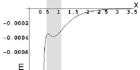
We stress that each of the field modes $\phi_{1}$ and $\phi_{2}$ on each own would produce an attractive force if the other was somehow turned off (e.g. by giving it very large mass). The repulsion seen in Fig. 2 may therefore be understood as an interference between the modes (or, more precisely, from the dependence of the interference term on the separation). As a side remark, we mention that the mathematics involved here is somewhat reminiscent to that of the Glashow- Iliopoulous-Maiani (GIM) mechanism [17], although actually applying it to quark mediated weak interactions would be, of course, completely unrealistic.

For a realistic way to obtain such a model, consider e.g. objects situated inside a circular cylinder of radius $R$ as in Fig. 1. Standard mode expansion of a field leaving in this cylinder would reduce it to a series of 1d fields of masses $m_{n}=\zeta_{n}/R$ with $\zeta_{n,m}$ zeroes of Bessel functions $J_{m}$ and of each derivative for TM and TE modes respectively. Standard boundary conditions on the bodies would demand specific (shape dependent) combinations of the 1d fields to vanish.

The fact that for very large and for very small distances the force attracts is a general feature not special to the specific model. At very large distances $x\gg 1$ only the channels of lowest mass contribute to the force. Having only this single mass, the above no-go theorem applies and we obtain attraction. At very small distances $x\ll 1$ the integrand decays very slowly with $\omega$ so that most of the contribution to the force comes from very large frequencies $\omega\sim{1\over x}$. At such frequencies all the $k_{i}$’s become practically equal: $k_{i}=\sqrt{m_{i}^{2}+\omega^{2}}\sim\omega\;\forall i$ and our theorem again imply attraction.

(E.g. in the above model $E\simeq-{1\over 4\pi x}Polylog[2,{(\alpha\cdot\beta)^{2}\over\alpha^{2}\beta^{2}}]$.) At intermediate distances the force may however change sign as the above example demonstrates.

It should be remarked however that this reasoning relies on the assumption of having only finitely many channels. In an infinite channel system it is conceivable that as $x$ becomes smaller more and more new channels (of higher $m$) become relevant, making the above argument false.

The short distance attraction argument may also become false in case the reflection coefficients decay very rapidly as $\omega\rightarrow\infty$. Also we remark that using fine tuning one might be able to construct a model where the leading short distance attractive term vanishes, in which case the resultant force can remain repulsive down to $x=0$. For example: Suppose one constructs a model where the $\alpha$’s and $\beta$’s depend on $\omega$ in such a way that $\tilde{\alpha},\tilde{\beta}$ are constants and take ($n=2$) $\alpha_{2}/\alpha_{1}=-\beta_{2}/\beta_{1}=1,m_{1}=0,m_{2}\neq 0$ then the attractive term which usually dominates at $x\rightarrow 0$ vanishes and the next to leading term result in a force which is attractive down to $x=0$. However any slight change of the parameters will make the usual leading term re-appear and thus turn the force into an attractive one (at $x=0$).

Our next repulsive example shows that for $d>1$ non-locality of dielectric functions, may also, in principle, result in repulsive behavior. The effect of spatial dispersion on Casimir forces between metals has been of interest for some time [16, 19]. It is particularly important in metals where long range density correlations in the medium can be present and substantially change the scaling of the force [20].

Our example here is very different from the situations considered in the references above. Our toy model is based on so called ”separable potentials”. Such potentials arise in variety of situations in physics and in mathematics, and were first introduced for Casimir type problems by Jaffe and Williamson [18]. They correspond to ”rank 1” perturbations, and can be written as $V=|f\rangle\langle f|$ for some function $f$, or in $x$ space notation as $V(x,x^{\prime})=f(x)f^{*}(x^{\prime})$. Such separable potentials describe the interactions involved in Feschbach resonances, and play a major role in the properties of fermi condensates. Note, also, that such $V$ is a positive operator by construction since $\langle\psi|V|\psi\rangle=|\langle\psi|f\rangle|^{2}>0$ for any $\psi$.

The situation we consider is of a scalar field, which can tunnel into traps where it has a bound state Fig. 3. Thus, in our case the perturbations are traps. Integrating out degrees of freedom in these traps will generate a perturbation of the form $\int{\rm d}x{\rm d}x^{\prime}\phi(x)t(x)G_{bound}(x,x^{\prime})t^{*}(x^{\prime})\phi(x^{\prime})$ for the field outside the trap, where $G_{bound}$ is the green’s function of the trap, and $t(x)$ is the tunnelling element.

Close to resonance, $G_{bound}$ may be approximated as: $G_{bound}\sim{f_{b}(x)f_{b}^{*}(x^{\prime})\over E-E_{b}}$ where $f_{b}$ is the wave function of a bound state, and when $E$ is close to $E_{b}$. Thus, the effective interaction with the trap is through the separable potential $V=f(x)f^{*}(x^{\prime})$, where $f(x)=\sqrt{{1\over|E-E_{b}|}}t(x)f_{b}(x)$.

For such potentials, one may readily calculate the $T$ operators, which turn out to be also of rank one, and so the interaction energy is easily calculated (One may also look at sums of separable potentials, corresponding to finite rank perturbations, which can be computed in the same way).

In case the free field interacts with the perturbation $V_{bound}\propto|f\rangle\langle f|$. We have:

And so,

thus, since the (positive) terms ${1\over 1+\langle f_{A}|G_{0}|f_{A}\rangle}{1\over 1+\langle f_{B}|G_{0}|f_{B}\rangle}$ do not depend on the distance, to find the direction of the force it is enough to consider $|\langle f_{B}|G_{0}|f_{A}\rangle|$.

As an example, we consider the following functions ²² 2 To avoid difficulties associated with $\delta$-function potential in 3d one should actually assume slightly smeared $\delta$-function. :

Taking also: $\alpha_{1}=1,\alpha_{2}=-4,\beta_{1}=1,\beta_{2}=-1$ we get a repulsive regime as shown in Fig. 4.

To summarize, we gave a general rule for the sign of the Casimir force at large distances and considered mechanisms allowing the force to reverse its direction at shorter distance. We have shown that such behavior is possible when an interaction is introduced between fields with different dispersion relations. Such a situation may mimic the interaction between bodies confined in an infinite cylinder which serves to quantize the transverse modes, rendering a quasi 1d situation. Secondly, we have shown that non-locality of a dielectric function may, in an extreme limit, result in repulsive behavior. This type of non-locality, typical of separable potentials, may arise in situations where the bodies represent ”traps” into which the field can tunnel, and interact with a bound state.

Acknowledgments: We would like to thank the KITP for hospitality during part of this work, as well as partial support from the NSF under Grant No. PHY05-51164. We also thank R. L. Jaffe for discussions and useful comments regarding separable potentials.

References

- [1] A. Lambrecht, M.-T. Jaekel and S. Reynaud, Phys.Lett. A225 (1997) 188-194.
- [2] O. Kenneth and I. Klich, Phys. Rev. Lett. 97, 160401 (2006).
- [3] T. H. Boyer, Phys. Rev. 174, 1764 (1968).
- [4] E. Elizalde and A. Romeo, Am. J. Phys. 59, 8 711(1991).
- [5] C. P. Bachas, quant-ph/0611082
- [6] F. M. Schmidt and H. W. Diehl, Phys. Rev. Lett. 101, 100601 (2008)
- [7] G. Feinberg and J. Sucher, Phys. Rev. A 2, 2395 (1970).
- [8] T. H. Boyer, Phys. Rev. A 9 2078 (1974).
- [9] D. T. Alves, C. Farina and A. C. Tort, Phys. Rev. A 61,034102 (2000).
- [10] J. C. da Silva, A. Matos neto, H. Q. Placido, M Revzen and A. E. Santana, Physica A 292, 411 (2001).
- [11] R. Balian and B. Duplantier, Ann. Phys.N.Y. 112, 165, (1978).
- [12] R. Golestanian, Phys. Rev. Lett. 95, 230601 (2005).
- [13] O. Kenneth and I. Klich, Phys. Rev. B 78, 014103 (2008).
- [14] Kimball A. Milton and J. Wagner J. Phys. A 41: 155402 ,2008.
- [15] O. Kenneth hep-th/9912102 M. T. Jaekel and S. Reynaud, J. Phys. I 1, 1395 (1991). quant-ph/0101067. C. Genet, A. Lambrecht, and S. Reynaud, Phys. Rev. A 67, 043811 (2003). van Kampen, N. G.; Nijboer, B. R. A.; Schram, K. Physics Letters A, Volume 26, Issue 7, p. 307-308.
- [16] E. I. Kats, Sov. Phys. JETP 46, 109 (1977).
- [17] S. L. Glashow, J. Iliopoulous and L.Maiani, Phys. Rev. D2 1285(1970).
- [18] R.L. Jaffe, L.R. Williamson, Annals Phys. 282 (2000) 432-448
- [19] Bo E. Sernelius, Phys. Rev. B 71, 235114 (2005); G. L. Klimchitskaya and V. M. Mostepanenko, Phys. Rev. B 75, 036101 (2007); Bo E. Sernelius, Phys. Rev. B 75, 036102 (2007)
- [20] J. F. Dobson, A. White, and A. Rubio, Phys. Rev. Lett. 96, 073201 (2006)