Time warps

The usual approach to extra dimensions in string theory is to consider a direct product,

$\displaystyle{ds_{10}^{2}=-dt^{2}+d\vec{x}^{2}+d\tilde{s}_{6}^{2}\,,}$

(1)

where $d\tilde{s}_{6}^{2}$ is, for example, the metric of a Calabi-Yau three-fold, as in [1]. This metric has the symmetries of Minkowski space, ${\bf R}^{3,1}$: translation invariance in the $t$ and $\vec{x}=(x^{1},x^{2},x^{3})$ directions, and also rotation and boost invariance.

A large literature has grown up on the study of “warped compactifications” of string theory: for a review, see [2]. A common way to write the metric ansatz is

$\displaystyle{ds_{10}^{2}=e^{2A(y)}\left[-dt^{2}+d\vec{x}^{2}\right]+e^{-2A(y)}d\tilde{s}_{6}^{2}\,,}$

(2)

where $y$ denotes, collectively, the coordinates involved in the metric $d\tilde{s}_{6}^{2}$. This is usually thought to be the most general ansatz consistent with the symmetries of ${\bf R}^{3,1}$.

It is less than straightforward to construct solutions of string theory of the form (2) where the extra-dimensional manifold is compact, because of a constraint from the strong energy condition [3, 4]:¹¹ 1 If we define $\tilde{T}_{MN}=T_{MN}-{1\over d-2}g_{MN}T^{L}_{L}$ in a $d$-dimensional theory, then the strong energy condition says that $\tilde{T}_{MN}\xi^{M}\xi^{N}\geq 0$ when $\xi^{M}$ is timelike or null. Assuming the Einstein equations, $R_{MN}=\kappa_{d}^{2}\tilde{T}_{MN}$, hold, this means that $R_{MN}\xi^{M}\xi^{N}\geq 0$. In particular, $R^{00}\geq 0$ when the metric is diagonal.

$\displaystyle{R^{00}=\tilde{\mathop{\rm\Box}}\nolimits A\geq 0\,,}$

(3)

where $\tilde{\mathop{\rm\Box}}\nolimits$ is the laplacian built from the metric $d\tilde{s}_{6}^{2}$. The problem is that the integral of $\tilde{\mathop{\rm\Box}}\nolimits A$ over the compact manifold vanishes, which can only happen if the inequality is saturated everywhere, meaning that the function is harmonic. And a harmonic function on a compact manifold must be constant. A resolution is to use orientifold planes: for example, O3-planes, as in [5]. Near an O3-plane, the geometry is ill-defined: formally, $e^{-4A}$ becomes negative.

One could consider a more general ansatz:

$\displaystyle{ds_{10}^{2}=e^{2A(y)}\left[-h(y)dt^{2}+d\vec{x}^{2}\right]+ds_{6}^{2}\,.}$

(4)

This has all the same symmetries as before, except for boost invariance. Boost invariance is quite well established experimentally (for a review, see for example [6]), so one might dismiss the ansatz (4) as obviously unacceptable. But suppose, for some reason, we are constrained to live at a particular value of $y$, call it $y_{*}$; or perhaps we are restricted to some narrow range of values of $y$ close to $y_{*}$ where $h$ is nearly constant. Then we would perceive the world to be boost-invariant (or nearly so), with a speed of light $c=\sqrt{h(y_{*})}$. If $h(y)>h(y_{*})$ away from $y_{*}$, then a particle that can propagate into the extra dimensions can appear to move superluminally from the point of view of an observer at $y_{*}$, in the sense that in a coordinate time $\Delta t$, the particle could propagate significantly further than $\sqrt{h(y_{*})}\Delta t$ without violating causality in the extra-dimensional geometry.

The ideas in the previous paragraph have a long history, which I will trace only partially here. Metrics of approximately the form (4) were discussed as early as [7], with a qualitative hint arising even in [8]; and the special case $A=0$ was treated in [9]. Time dependent versions were studied in [10, 11] in an effort to use a variable speed of light to solve cosmological problems without inflation, along the lines of [12, 13]. Further work in the direction of a variable speed of light has been reviewed in [14], and the extensive topic of brane world cosmology has been reviewed in [15]. Five-dimensional metrics similar to (4) were termed “asymmetrically warped spacetimes” in [16], where, in the spirit of earlier work [17, 18, 19, 20], the examples of five-dimensional AdS-Schwarzschild and Reissner-Nordström-AdS were discussed. It was noted in [16] that one needs $w<-1$ on the Planck brane. The need for a violation of the null energy condition was later demonstrated more generally [21], using an argument which I extend in this paper. Special cases of (4) where $A=0$ were discussed in [22], and also in [23] as part of an approach to the cosmological constant problem using the model of [24]. Some general constraints on asymmetrically warped string theory constructions were considered in [25]. More explicit string theory constructions have been considered, for example in [26].

Returning to the ansatz (4): It’s difficult to arrange for non-constant $h(y)$ over a compact extra-dimensional manifold because of a constraint arising from the null energy condition:²² 2 The null energy condition says $T_{MN}\xi^{M}\xi^{N}\geq 0$ for all null vectors $\xi^{M}$. Assuming the Einstein equations hold, this means $R_{MN}\xi^{M}\xi^{N}\geq 0$. In particular, $-R^{0}_{0}+R^{1}_{1}\geq 0$ when the metric is diagonal.

$\displaystyle{4h^{2}e^{-2A}(-R^{0}_{0}+R^{1}_{1})=-3\tilde{g}^{mn}\partial_{m}h\partial_{n}h+\tilde{\mathop{\rm\Box}}\nolimits(h^{2})\geq 0\,.}$

(5)

Integrating over the compact manifold (and supposing $e^{-2A}$ is for some reason well-defined everywhere), one would be forced by the inequality to conclude that $h$ is constant. This argument is in the same spirit as [21], but it generalizes more easily to (almost) any dimension, as we will see in section 2. In contrast to the situation described by (3), I do not know an explicit string theory construction that would evade the no-go argument based on (5). However, one may temporarily ignore this argument by considering non-compact extra dimensions. This amounts to turning off gravity, because the wave-function of the four-dimensional graviton is non-normalizable in the extra dimensions.

The simplest sort of non-compact asymmetrically warped geometry is just an extra-dimensional black brane. For example, the near-extremal D3-brane has a metric of the form (4) with

$\displaystyle{d\tilde{s}_{6}^{2}=e^{-2A(y)}\left({dy^{2}\over h(y)}+y^{2}d\Omega_{5}^{2}\right)\,,}$

(6)

where now $y$ is a single real variable, $d\Omega_{5}^{2}$ is the metric on a unit $S^{5}$, and

$\displaystyle{e^{-4A(y)}=1+{L^{4}\over y^{4}}\qquad\qquad h(y)=1-{y_{0}^{4}\over y^{4}}\,.}$

(7)

A difficulty is that the existence of a regular horizon at $y=y_{0}$ is associated with a finite Hawking temperature,

$\displaystyle{T={1\over\pi y_{0}}\left(1+{L^{4}\over y_{0}^{4}}\right)^{-1/2}\,.}$

(8)

Following [18], we might imagine our world as a brane at some fixed value of $y$ in the geometry (6). Certainly, such a construction would lead to an observed speed of light which is slower than what can be attained far from the D3-branes. But the finite temperature (8) makes the construction seem less interesting, because it means we are not describing the ground state. Likewise, as emphasized in [27], the $AdS_{5}$-Schwarzschild and $AdS_{5}$-Reissner-Nordström geometries considered in [16] do not describe ground states, but instead finite temperature states of a strongly coupled conformal theory. An exception is the extremal $AdS_{5}$-Reissner-Nordström solution, which has zero temperature; but it still has a macroscopic Bekenstein-Hawking entropy, meaning that it doesn’t describe a single physical state, but instead a large ensemble of states. This may not be fatal, but entropic solutions do not seem to me the best of starting points when seeking to describe the vacuum.

I wish to consider in this paper a subclass of asymmetrically warped solutions which, by requirement, have no temperature and no entropy. I will refer to such backgrounds as “time warps.” A simple way to construct one is to cut off a black brane background above the horizon, as was indeed considered in [16, 28]. I will instead work with five-dimensional variants of the geometries found in [29] in asymptotically $AdS_{4}$ geometries, using the abelian Higgs model coupled to gravity. This model, first considered in [30], has the following action:

$\displaystyle{S_{\rm bulk}={1\over 16\pi G_{D+1}}\int d^{D+1}x\,\sqrt{g}{\cal L}_{\rm bulk}\,,}$

(9)

where

$\displaystyle{{\cal L}_{\rm bulk}=R-{1\over 4}F_{\mu\nu}^{2}-|(\partial_{\mu}-iqA_{\mu})\psi|^{2}-V(|\psi|)\,.}$

(10)

For appropriate choices of $V(|\psi|)$ and $q$, the classical equations of motion following from (9) admit superconducting black hole solutions [30, 31, 32, 33], which spontaneously break the $U(1)$ gauge symmetry in the bulk. See [34] for earlier work on superconducting black holes; [35, 36] for earlier work on the possible relation between black holes in $AdS_{4}$ and phases of superconducting materials; [37, 38], among others, for discussion of variants on this type of solution and dual superfluids; and [39] for an overview and further references.

The focus on four-dimensional anti-de Sitter space in the superconducting black hole literature has been driven by the interest in strongly coupled $2+1$-dimensional conformal field theories, which has been driven in turn by the hope of explaining phenomena in thin-film or layered superconductors in terms of quantum critical points.³³ 3 An exception is [40], which deals with five-dimensional geometries. Also there have been studies of superconducting black holes based on the Einstein-Yang-Mills lagrangian in four [41, 42, 43] and higher [44] dimensions. In this paper I will focus instead on five-dimensional geometries, because they provide a minimal example of non-compact time warp geometries that include a copy of ${\bf R}^{3,1}$. By minimal, I mean that there is only one extra dimension, and the field content appears to be the minimal one that can support a time warp. I will find the geometries using the same strategy as in [29]. And as in [29], the time warp geometries I find are domain walls with conformal invariance in the ultraviolet (UV) and infrared (IR) regions of the bulk, but different speeds of light as measured by a fixed coordinate system on the boundary. One therefore expects that correlation functions interpolate between a conformally invariant form in the ultraviolet, and a different conformally invariant form—characterized by a different speed of light—in the infrared.

The rest of this paper is organized as follows. In section 2 I exhibit the time warp geometry which I focus on. In section 3 I calculate the spectral measure of two-point correlators for a massive scalar propagating in the time warp geometry. I relate this spectral measure to unparticle phase space and explain how time warp effects could manifest themselves in the decay of a heavy particle into a light visible particle plus unparticle stuff. An appendix contains some additional technical detail on the computation of two-point functions. In section 4, I consider what it would take to “compactify” the asymptotically $AdS_{5}$ time warp geometries using a Planck brane construction.⁴⁴ 4 “Compactify” is a slight misnomer here because after introducing the Planck brane, the geometry is still non-compact in the infrared, as in [17]. It is like a true compactification in that there is a finite five-dimensional volume below any finite four-volume element on the Planck brane. As one might anticipate based on the no-go argument discussed around (5), I am forced to entertain a theory on the brane which violates the null energy condition. In section 5, I show that it is possible to obtain an four-dimensional infrared-massless graviton by including a wrong-sign Einstein-Hilbert term in the action of the Planck brane. Altogether, it must be admitted that the Planck brane construction is peculiar.

I will construct a solution to the classical equations of motion of the Abelian Higgs model in $AdS_{5}$, starting with the ansatz

$\displaystyle{ds_{5}^{2}=e^{2A(r)}\left[-h(r)dt^{2}+d\vec{x}^{2}\right]+e^{2B(r)}dr^{2}\,.}$

(11)

$B(r)$ parametrizes the gauge freedom of choosing different radial variables. Let us pass to the gauge $B=-{1\over 2}\log h$, where the equations of motion and constraints are simplest to state. Rotational invariance in the $\vec{x}$ directions forces $A_{i}=0$ for $i=1,2,3$. Let’s also assume $A_{r}=0$ (which is a gauge choice) and use $\Phi$ to denote $A_{0}$. Finally, let’s restrict attention to solutions where $\psi$ is real. The equations of motion are

	$\displaystyle A^{\prime\prime}$	$\displaystyle=$	$\displaystyle-{1\over 3}|\psi^{\prime}|^{2}-{e^{-2A}\over 3h^{2}}q^{2}\Phi^{2}|\psi|^{2}$		(12a)
	$\displaystyle h^{\prime\prime}+4A^{\prime}h^{\prime}$	$\displaystyle=$	$\displaystyle e^{-2A}\left(\Phi^{\prime 2}+{2\over h}q^{2}\Phi^{2}|\psi|^{2}\right)$		(12b)
	$\displaystyle\Phi^{\prime\prime}+2A^{\prime}\Phi^{\prime}$	$\displaystyle=$	$\displaystyle{2\over h}q^{2}\Phi|\psi|^{2}$		(12c)
	$\displaystyle\psi^{\prime\prime}+\left(4A^{\prime}+{h^{\prime}\over h}\right)\psi^{\prime}$	$\displaystyle=$	$\displaystyle-{e^{-2A}\over h^{2}}q^{2}\Phi^{2}\psi+{1\over h}{\partial V\over\partial\psi^{*}}\,.$		(12d)

The constraint coming from the $G_{rr}$ Einstein equation is

$\displaystyle{24h^{2}A^{\prime 2}+6hh^{\prime}A^{\prime}+e^{-2A}h\Phi^{\prime 2}-2h^{2}|\psi^{\prime}|^{2}-2e^{-2A}q^{2}\Phi^{2}|\psi|^{2}+2hV=0\,.}$

(13)

An additional first-order equation can be extracted by noticing that the quantity

$\displaystyle{Q=e^{4A}(h^{\prime}-e^{-2A}\Phi\Phi^{\prime})}$

(14)

is a constant if the equations (12) and (13) are obeyed. Assuming that the infrared geometry is asymptotically $AdS_{5}$ amounts to assuming that $Q=0$. This is because both $h^{\prime}$ and $\Phi^{\prime}$ must go to zero in the infrared, while $h$ remains non-zero and $\Phi$ is bounded. Solutions with a regular horizon typically have $Q\neq 0$. So $Q=0$ is a sort of extremality condition.⁵⁵ 5 The existence of the conserved charge (14) and its relevance to extremal solutions were pointed out to me by A. Nellore. In a more general gauge where $B$ is left as an unspecified function of $r$ but $A_{r}$ is still constrained to vanish, $\displaystyle{Q={e^{4A-B}\over\sqrt{h}}(h^{\prime}-e^{-2A}\Phi\Phi^{\prime})\,.}$ (15) It may seem puzzling that $Q$ isn’t invariant under shifts of $\Phi$ by a constant, given that such shifts preserve the more general gauge just described. However, after such a shift, the complex scalar $\psi$ would have a time-dependent phase. Requiring $\psi$ to be time-independent thus disallows shifts of $\Phi$ by a constant—unless $\psi=0$. If in fact $\psi=0$, then there is an additional conserved quantity, ${e^{2A-B}\over\sqrt{h}}\Phi^{\prime}$. Shifting $\Phi$ by an additive constant causes $Q$ to change by some multiple of this quantity.

Already from (12a) and (12b) one can see the no-go theorem of [21] at work, as well as a application of the $c$-theorem argument of [45]. In brief: the left-hand side of (12a) is proportional to $R^{0}_{0}-R^{r}_{r}$, so the right hand side has to be negative according to the null energy condition. Thus $A$ is superharmonic as a function of $r$, which means it can’t have a minimum unless one introduces an additional matter source. The left-hand side of (12b) is proportional to $R^{1}_{1}-R^{0}_{0}$, so the right hand side has to be positive, again according to the null energy condition. Thus $h$ is subharmonic with respect to the line element $d\tilde{s}^{2}=e^{-8A}dr^{2}$ in the $r$ direction, indicating that it cannot have a maximum without some additional matter source as long as $A$ is well defined. As argued in [29], (12a) and (12b) also imply that for backgrounds which are asymptotically anti-de Sitter, the effective speed of light $\sqrt{h(r)}$ increases from the infrared to the ultraviolet.⁶⁶ 6 There appears to be some tension between (3), which indicates that $A$ is subharmonic in a ten-dimensional compactification, and (12a), which shows that it is superharmonic in five. To understand the situation more comprehensively, consider a $D$-dimensional ansatz $\displaystyle{ds_{D}^{2}=e^{2A}(-hdt^{2}+d\vec{x}^{2})+e^{2B}d\tilde{s}_{D-4}^{2}\,,}$ (16) where $A$, $B$, and $h$ depend only on the $D-4$ coordinates of $d\tilde{s}^{2}_{D-4}$. Setting $h=1$, $D\neq 6$, and $B={4\over 6-D}A$, one finds $\displaystyle{-e^{2B}R^{0}_{0}=\tilde{\mathop{\rm\Box}}\nolimits A\,,}$ (17) and the strong energy condition says this should be positive. Both the strong energy condition and the null energy condition are satisfied by the stress tensor following from (10). Indeed, if $h=1$ and $D=5$, $A$ is superharmonic with respect to the metric $dr^{2}$ and subharmonic with respect to the metric $e^{8A}dr^{2}$. Using the same ansatz (16), assuming $D\neq 6$, and setting $B={4\over 6-D}A$, one finds that $\displaystyle{4h^{2}e^{2B}(-R^{0}_{0}+R^{1}_{1})=-3\tilde{g}^{mn}\partial_{m}h\partial_{n}h+\tilde{\mathop{\rm\Box}}\nolimits(h^{2})\,.}$ (18) So the argument around (5) survives essentially unchanged for dimensions $D\neq 6$. It is notable that both lines of argument discussed in this footnote have no force for $D=6$. It would be interesting to consider six-dimensional time warps in more detail.

Unfortunately, I don’t know a choice of the scalar potential that leads to analytically tractable equations of motion, even in the presence of the extremality constraint $Q=0$. So I will solve them numerically for particular choices of parameters. Specifically, I will choose

$\displaystyle{V=-{12\over L^{2}}+m^{2}|\psi|^{2}+{u\over 2}|\psi|^{4}\,,}$

(19)

with $m^{2}<0$ and $u>0$. With this choice, the infrared geometry is itself anti-de Sitter, but with a different radius, $L_{\rm IR}$, determined through the equation $V(\psi_{\rm IR})=-12/L_{\rm IR}^{2}$, where $\psi_{\rm IR}=\sqrt{-m^{2}/u}$ is the $U(1)$ symmetry-breaking extremum of the potential. The infrared copy of $AdS_{5}$ signals emergent conformal symmetry: emergent in the sense that it arises only in the infrared limit of the dual field theory. It was speculated in [29] that scalar potentials which have no minima lead to emergent Lorentz symmetry in the infrared, rather than emergent conformal symmetry. Evidence in favor of this conjecture has appeared in [33].

For numerical work, I found that the most convenient gauge is $B=0$, instead of the gauge $B=-{1\over 2}\log h$ that I used in (12)-(14). In the $B=0$ gauge, $A^{\prime\prime}$ does not have a definite sign. However, $A^{\prime}=1/L$ in the UV and $A^{\prime}=1/L_{\rm IR}$ in the IR.

The ultraviolet dimension of the operator dual to $\psi$ is

$\displaystyle{\Delta_{\psi}^{\rm UV}=2+\sqrt{4+m^{2}L^{2}}\,.}$

(20)

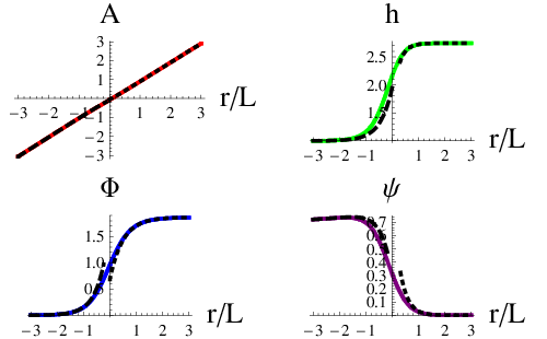
Provided $-4\leq m^{2}L^{2}$, the asymptotically $AdS_{5}$ geometry is stable [46, 47]. If also $m^{2}L^{2}\leq 0$, then one does not have to stipulate boundary conditions on $\psi$ at the conformal boundary. However, one may do so, and in studying solutions to (12), I generally did: I required $\psi\propto e^{-\Delta_{\psi}^{\rm UV}A}$ rather than $\psi\propto e^{(\Delta_{\psi}^{\rm UV}-4)A}$. My choice corresponds to requiring that the breaking of the $U(1)$ symmetry associated with the phase of $\psi$ is spontaneous rather than explicit in the dual conformal theory.⁷⁷ 7 It is well understood [48] that for the range $-4\leq m^{2}L^{2}<-3$, one can replace $\Delta_{\psi}^{\rm UV}\to 4-\Delta_{\psi}^{\rm UV}$; this corresponds to a new CFT, from which the original can be recovered from a renormalization group flow triggered by double-trace terms. It is even possible to make sense of more general boundary conditions on $\psi$ in terms of multi-trace operators [49]. With this choice (or with any definite choice of boundary conditions on $\psi$), according to the same reasoning as in [29], there can be at most discretely many solutions with $h$ nowhere vanishing. In instances where I was able to find more than one solution, the one with no nodes in $\psi$ had the smallest value of $h$ in the UV.⁸⁸ 8 For example, the choice of parameters (21) leads to one solution with $h_{\rm UV}\approx 2.74$, which I will describe in some detail, and another with $h_{\rm UV}\approx 34.0$, in which $\psi$ has a single node. I will assume that solutions with no nodes (or as few nodes as possible) in $\psi$ are preferred; however, this is just an assumption. In figure 1, I exhibit the solution I found for the following choice of parameters:

$\displaystyle{qL=3\qquad m^{2}L^{2}=-2\qquad uL^{2}=4\,.}$

(21)

In the solution I found for this choice of parameters, the speed of light is about $1.7$ times faster in the ultraviolet part of the geometry (large positive $r$) than in the infrared part (large negative $r$). With the choice of parameters (21), it happens that $L_{\rm IR}$ and $L$ are quite close together: $L_{\rm IR}/L\approx 0.97$.

It is possible to generate series expansions in the infrared and the ultraviolet for the solution I have described. In the infrared,

	$\displaystyle A$	$\displaystyle=$	$\displaystyle{r\over L_{\rm IR}}+\ldots$		(22a)
	$\displaystyle h$	$\displaystyle=$	$\displaystyle 1+{\Delta^{\rm IR}_{\Phi}-2\over\Delta^{\rm IR}_{\Phi}-3}\Phi_{1}^{2}e^{2(\Delta_{\Phi}^{\rm IR}-3)r/L_{\rm IR}}+\ldots$		(22b)
	$\displaystyle\Phi$	$\displaystyle=$	$\displaystyle\Phi_{1}e^{(\Delta_{\Phi}^{\rm IR}-2)r/L_{\rm IR}}+\ldots$		(22c)
	$\displaystyle\psi$	$\displaystyle=$	$\displaystyle\psi_{\rm IR}+\psi_{1}e^{(\Delta_{\psi}^{\rm IR}-4)r/L_{\rm IR}}+\ldots\,,$		(22d)

where $\ldots$ denotes terms that are exponentially smaller in the infrared than the ones shown. Here

$\displaystyle{\Delta_{\Phi}^{\rm IR}}$ $\displaystyle{{}=1+\sqrt{1+2q^{2}\psi_{\rm IR}^{2}}L_{\rm IR}^{2}}$ $\displaystyle{\Delta_{\psi}^{\rm IR}}$ $\displaystyle{{}=2+\sqrt{4+(m^{2}+3u\psi_{\rm IR}^{2})L_{\rm IR}^{2}}\,,}$

(23)

and the solution I exhibited has

$\displaystyle{\Phi_{1}=1\qquad\psi_{1}=0.168\,.}$

(24)

(A scaling symmetry, $x^{m}\to\lambda x^{m}$ while $r\to r-L_{\rm IR}\log\lambda$ and $\Phi\to\Phi/\lambda$, allows one to set $\Phi_{1}=1$ provided it is non-zero.) In the ultraviolet,

	$\displaystyle A$	$\displaystyle=$	$\displaystyle{r\over L}+a_{1}-{p_{1}p_{2}\over 16h_{\rm UV}}e^{-4r/L}+\ldots$		(25a)
	$\displaystyle h$	$\displaystyle=$	$\displaystyle h_{\rm UV}+{p_{1}p_{2}\over 2}e^{-4r/L}+\ldots$		(25b)
	$\displaystyle\Phi$	$\displaystyle=$	$\displaystyle p_{1}+p_{2}e^{-2r/L}+\ldots$		(25c)
	$\displaystyle\psi$	$\displaystyle=$	$\displaystyle s_{2}e^{-\Delta_{\psi}^{\rm UV}r/L}+\ldots\,,$		(25d)

where $\ldots$ indicates terms which are exponentially smaller in the ultraviolet than the ones shown. The solution I exhibited has

$\displaystyle{a_{1}=-0.0963\qquad h_{\rm UV}=2.74\qquad p_{1}=1.86\qquad p_{2}=-1.18\qquad s_{2}=0.955\,.}$

(26)

The asymptotics shown in figure 1 are based on (22) and (25), but in some cases evaluated to higher orders and with greater numerical precision.

If we think of the UV speed of light as the ordinary one of daily experience, then the asymptotically anti-de Sitter geometry can be interpreted as describing a medium with a definite index of refraction. Low-energy signals pass through the infrared part of the geometry, where they can only go at a fraction of the UV speed of light.

A more tantalizing possibility is that the physics of our world can be described as the infrared physics in a time warp geometry. Then the speed of light that we measure is the infrared speed of light. We are, in effect, caught in the refractive medium. If only we could pass through the domain wall and get into the UV part of the geometry, then we could move superluminally from the perspective of an infrared observer.

As a first step toward exploring the phenomenology of time warps, I consider in this section how relativistic kinematics is altered for the field theory dual to the type of non-compact time warp constructed in section 2. Because such a geometry is asymptotically $AdS_{5}$, one can extract two-point correlators for operators in the dual field theory. This field theory is strongly coupled, so it is not straightforward to make a comparison with perturbative quantum field theory. What is straightforward is to make a connection with recent ideas about “unparticle physics” [50], which is the possibility that an approximately conformal, strongly coupled sector—the unparticles—will be discovered through high-energy collisions, for example at the LHC. In section 3.1, without reference to time warps, I review the connection between the imaginary part of the two-point Green’s functions in a conformal field theory and the phase space for unparticles. Then, in section 3.2, I calculate in a specific example how this phase space gets modified by time warp effects.

Adding a Planck brane means adding a term to the action:

$\displaystyle{S=S_{\rm bulk}+S_{\rm brane}\,,}$

(45)

where

$\displaystyle{S_{\rm brane}={1\over 16\pi G_{5}}\int d^{4}x\,\sqrt{h}{\cal L}_{\rm brane}\,,}$

(46)

and $h_{mn}$ is the induced metric on the brane. This extra term results in additional terms in the equations of motion which are distributions supported at the position of the brane, say at $r=0$. For purposes of calculation, it is convenient to think of two mirror-image copies of the bulk geometry separated by the Planck brane. This can be thought of as the “upstairs” picture of a ${\bf Z}_{2}$ orbifold acting as $r\to-r$. Such a picture is well-motivated from string theory [62, 63, 64, 65, 66] and has been widely considered following [17]. Indeed, most of the earlier works on asymmetrically warped geometries summarized in section 1 employ a Planck brane. Some of the results of this section are quite standard: for example the junction conditions on the metric components are special cases of more general relations derived in [67]. However, in contrast to [16], I assign positive parity to the ${\bf R}^{3,1}$ components of $A_{\mu}$ under the ${\bf Z}_{2}$ orbifold symmetry and negative parity to $A_{r}$.

For simplicity, I will work in the following axial gauge throughout this section:

$\displaystyle{ds_{5}^{2}=g_{mn}dx^{m}dx^{n}+dr^{2}\qquad A=A_{m}dx^{m}\,,}$

(47)

where $m$ and $n$ run from $0$ to $3$. The metric coefficients $g_{mn}$, the gauge field components $A_{m}$, and the scalar $\psi$ may depend on $r$ as well as $x^{m}$. It will be convenient to define a unit normal $n_{\mu}dx^{\mu}=dr$ to the brane, where, as usual, $\mu$ runs over all five dimensions of the bulk. Then one may express the induced metric as a $5\times 5$ tensor as $h_{\mu\nu}=g_{\mu\nu}-n_{\mu}n_{\nu}$. In the following, I will pass freely between four- and five-dimensional forms of tensors on the brane whose components in the $\mu=5$ direction vanish.

The equations of motion resulting from (45) are

$\displaystyle{G_{\mu\nu}}$ $\displaystyle{{}={1\over 2}T_{\mu\nu}^{\rm bulk}+{1\over 2}T_{\mu\nu}^{\rm brane}\delta(r)}$ $\displaystyle{\nabla_{\mu}F^{\mu\nu}}$ $\displaystyle{{}=J^{\nu}_{\rm bulk}+J^{\nu}_{\rm brane}\delta(r)}$ $\displaystyle{D_{\mu}D^{\mu}\psi}$ $\displaystyle{{}={\partial V\over\partial\psi^{*}}+j^{\rm brane}\delta(r)\,,}$

(48)

where

$\displaystyle{T_{\mu\nu}^{\rm bulk}}$ $\displaystyle{{}=2D_{\mu}\psi^{*}D_{\nu}\psi-|D\psi|^{2}g_{\mu\nu}-Vg_{\mu\nu}+F_{\mu\alpha}F_{\nu}{}^{\alpha}-{1\over 4}g_{\mu\nu}F_{\alpha\beta}^{2}}$ $\displaystyle{J_{\mu}^{\rm bulk}}$ $\displaystyle{{}=iq(\psi^{*}\partial_{\mu}\psi-\psi\partial_{\mu}\psi^{*})+2q^{2}A_{\mu}|\psi|^{2}}$ $\displaystyle{D_{\mu}\psi}$ $\displaystyle{{}\equiv(\partial_{\mu}-iqA_{\mu})\psi}$

(49)

and the brane sources are defined by

$\displaystyle{\delta S_{\rm brane}={1\over 16\pi G_{5}}\int d^{4}x\,\sqrt{h}\left[{1\over 2}\delta h^{mn}T_{mn}^{\rm brane}-\delta A^{m}J_{m}^{\rm brane}-\delta\psi^{*}j^{\rm brane}-\delta\psi j^{\rm brane,*}\right]\,.}$

(50)

Assuming $g_{mn}$, $A_{m}$ and $\psi$ are smooth functions of $r$ except for jumps in the first derivatives at $r=0$, one can extract the brane source terms by integrating (48) over a small interval around $r=0$: for example,

$\displaystyle{T_{\mu\nu}^{\rm brane}=2\lim_{\epsilon\to 0+}\int_{-\epsilon}^{\epsilon}dr\,G_{\mu\nu}\,,}$

(51)

where I’ve omitted $T_{\mu\nu}^{\rm bulk}$ because it only involves first derivatives, which have no singular part. One easily finds

$\displaystyle{T_{\mu\nu}^{\rm brane}}$ $\displaystyle{{}=4\left[K_{\mu\nu}-Kh_{\mu\nu}\right]_{0^{-}}}$ $\displaystyle{J_{\mu}^{\rm brane}}$ $\displaystyle{{}=-2\left[F_{r\mu}\right]_{0^{-}}}$ $\displaystyle{j^{\rm brane}}$ $\displaystyle{{}=-2\left[\partial_{r}\psi\right]_{0^{-}}\,,}$

(52)

where in general,

$\displaystyle{\left[f(r)\right]_{0^{-}}\equiv\lim_{r\to 0^{-}}f(r)\,,}$

(53)

and the extrinsic curvature is

$\displaystyle{K_{\mu\nu}=-h_{\mu}{}^{\rho}\nabla_{\rho}n_{\nu}=-{1\over 2}{\partial h_{\mu\nu}\over\partial r}\,.}$

(54)

The middle expression in (54) is the defining equation for $K_{\mu\nu}$, and the last expression is a result of the gauge choice (47). $K$ denotes the trace $g^{\mu\nu}K_{\mu\nu}$. $K_{\mu r}=0$ for all $\mu$, and as a consequence, $T^{\rm brane}_{\mu r}=0$.

For brevity, let’s define

$\displaystyle{\epsilon=-T_{0}^{0,{\rm brane}}\qquad p={1\over 3}T_{i}^{i,{\rm brane}}\qquad\rho=J_{0}^{\rm brane}\qquad j=j^{\rm brane}\,,}$

(55)

where $i$ runs from $1$ to $3$. Plugging the ansatz (11) into (52) leads to

$\displaystyle{\epsilon=\left[12A^{\prime}\right]_{0^{-}}\qquad p=\left[-12A^{\prime}-{2h^{\prime}\over h}\right]_{0^{-}}\qquad\rho=\left[-2\Phi^{\prime}\right]_{0^{-}}\qquad j=\left[-2\psi^{\prime}\right]_{0^{-}}\,,}$

(56)

Thus we see that the Planck brane must carry electric charge under the gauge field $A_{\mu}$, and its stress tensor must also break Lorentz invariance.¹⁰¹⁰ 10 If I had assigned negative parity to $\Phi$, as in [16], then the boundary condition at the Planck brane would be $\Phi=0$. This cannot be reconciled with the requirement that $\Phi\to 0$ in the infrared part of the geometry. Perhaps some variant of the bulk solution could accommodate non-zero $\Phi$ in the infrared. But it would be impossible to recover Lorentz symmetry in the infrared with both $\Phi$ and $\psi$ non-zero there, because the conserved current $J_{\mu}=i\psi^{*}\vbox{\halign{#\cr$\leftrightarrow$\crcr\kern 0.0pt\cr$\hfil\displaystyle{\partial}\hfil$\crcr}}_{\mu}\psi+2q^{2}A_{\mu}\psi^{*}\psi$ coupled to $A_{\mu}$ has $J_{0}\neq 0$. If $\psi$ is zero in the infrared, then non-zero $\Phi$ is possible, but there is still some potential difficulty: the gauge field $A=\Phi dt$ is ill-defined as a 1-form at a horizon where $g^{tt}\to\infty$.

References

- [1] P. Candelas, G. T. Horowitz, A. Strominger, and E. Witten, “Vacuum Configurations for Superstrings,” Nucl. Phys. B258 (1985) 46–74.
- [2] M. R. Douglas and S. Kachru, “Flux compactification,” Rev. Mod. Phys. 79 (2007) 733–796, hep-th/0610102.
- [3] G. W. Gibbons, “Aspects of supergravity theories.” Three lectures given at GIFT Seminar on Theoretical Physics, San Feliu de Guixols, Spain, Jun 4-11, 1984.
- [4] J. M. Maldacena and C. Nunez, “Supergravity description of field theories on curved manifolds and a no go theorem,” Int. J. Mod. Phys. A16 (2001) 822–855, hep-th/0007018.
- [5] H. L. Verlinde, “Holography and compactification,” Nucl. Phys. B580 (2000) 264–274, hep-th/9906182.
- [6] D. Mattingly, “Modern tests of Lorentz invariance,” Living Rev. Rel. 8 (2005) 5, gr-qc/0502097.
- [7] G. Kaelbermann and H. Halevi, “Nearness through an extra dimension,” gr-qc/9810083.
- [8] V. A. Rubakov and M. E. Shaposhnikov, “Do We Live Inside a Domain Wall?,” Phys. Lett. B125 (1983) 136–138.
- [9] M. Visser, “An Exotic Class of Kaluza-Klein Models,” Phys. Lett. B159 (1985) 22, hep-th/9910093.
- [10] D. J. H. Chung and K. Freese, “Can geodesics in extra dimensions solve the cosmological horizon problem?,” Phys. Rev. D62 (2000) 063513, hep-ph/9910235.
- [11] D. Youm, “Brane world cosmologies with varying speed of light,” Phys. Rev. D63 (2001) 125011, hep-th/0101228.
- [12] J. W. Moffat, “Superluminary universe: A Possible solution to the initial value problem in cosmology,” Int. J. Mod. Phys. D2 (1993) 351–366, gr-qc/9211020.
- [13] A. Albrecht and J. Magueijo, “A time varying speed of light as a solution to cosmological puzzles,” Phys. Rev. D59 (1999) 043516, astro-ph/9811018.
- [14] J. Magueijo, “New varying speed of light theories,” Rept. Prog. Phys. 66 (2003) 2025, astro-ph/0305457.
- [15] D. Langlois, “Brane cosmology: An introduction,” Prog. Theor. Phys. Suppl. 148 (2003) 181–212, hep-th/0209261.
- [16] C. Csaki, J. Erlich, and C. Grojean, “Gravitational Lorentz violations and adjustment of the cosmological constant in asymmetrically warped spacetimes,” Nucl. Phys. B604 (2001) 312–342, hep-th/0012143.
- [17] L. Randall and R. Sundrum, “An alternative to compactification,” Phys. Rev. Lett. 83 (1999) 4690–4693, hep-th/9906064.
- [18] E. Kiritsis, “Supergravity, D-brane probes and thermal super Yang-Mills: A comparison,” JHEP 10 (1999) 010, hep-th/9906206.
- [19] S. H. S. Alexander, “On the varying speed of light in a brane-induced FRW universe,” JHEP 11 (2000) 017, hep-th/9912037.
- [20] P. Bowcock, C. Charmousis, and R. Gregory, “General brane cosmologies and their global spacetime structure,” Class. Quant. Grav. 17 (2000) 4745–4764, hep-th/0007177.
- [21] J. M. Cline and H. Firouzjahi, “No-go theorem for horizon-shielded self-tuning singularities,” Phys. Rev. D65 (2002) 043501, hep-th/0107198.
- [22] S. L. Dubovsky, “Tunneling into extra dimension and high-energy violation of Lorentz invariance,” JHEP 01 (2002) 012, hep-th/0103205.
- [23] C. Deffayet, G. R. Dvali, G. Gabadadze, and A. Lue, “Braneworld flattening by a cosmological constant,” Phys. Rev. D64 (2001) 104002, hep-th/0104201.
- [24] G. R. Dvali, G. Gabadadze, and M. Porrati, “4D gravity on a brane in 5D Minkowski space,” Phys. Lett. B485 (2000) 208–214, hep-th/0005016.
- [25] A. R. Frey, “String theoretic bounds on Lorentz-violating warped compactification,” JHEP 04 (2003) 012, hep-th/0301189.
- [26] O. J. Ganor, “A New Lorentz Violating Nonlocal Field Theory From String-Theory,” Phys. Rev. D75 (2007) 025002, hep-th/0609107.
- [27] P. Creminelli, “Holography of asymmetrically warped space-times,” Phys. Lett. B532 (2002) 284–290, hep-th/0111107.
- [28] J. M. Cline and L. Valcarcel, “Asymmetrically warped compactifications and gravitational Lorentz violation,” JHEP 03 (2004) 032, hep-ph/0312245.
- [29] S. S. Gubser and F. D. Rocha, “The gravity dual to a quantum critical point with spontaneous symmetry breaking,” 0807.1737.
- [30] S. S. Gubser, “Breaking an Abelian gauge symmetry near a black hole horizon,” 0801.2977.
- [31] S. A. Hartnoll, C. P. Herzog, and G. T. Horowitz, “Building an AdS/CFT superconductor,” 0803.3295.
- [32] S. A. Hartnoll, C. P. Herzog, and G. T. Horowitz, “Holographic Superconductors,” 0810.1563.
- [33] S. S. Gubser and A. Nellore, “Low-temperature behavior of the Abelian Higgs model in anti-de Sitter space,” 0810.4554.
- [34] S. S. Gubser, “Phase transitions near black hole horizons,” Class. Quant. Grav. 22 (2005) 5121–5144, hep-th/0505189.
- [35] S. A. Hartnoll, P. K. Kovtun, M. Muller, and S. Sachdev, “Theory of the Nernst effect near quantum phase transitions in condensed matter, and in dyonic black holes,” Phys. Rev. B76 (2007) 144502, 0706.3215.
- [36] S. A. Hartnoll and C. P. Herzog, “Ohm’s Law at strong coupling: S duality and the cyclotron resonance,” Phys. Rev. D76 (2007) 106012, 0706.3228.
- [37] P. Basu, A. Mukherjee, and H.-H. Shieh, “Supercurrent: Vector Hair for an AdS Black Hole,” 0809.4494.
- [38] C. P. Herzog, P. K. Kovtun, and D. T. Son, “Holographic model of superfluidity,” 0809.4870.
- [39] S. Sachdev and M. Mueller, “Quantum criticality and black holes,” 0810.3005.
- [40] G. T. Horowitz and M. M. Roberts, “Holographic Superconductors with Various Condensates,” 0810.1077.
- [41] S. S. Gubser, “Colorful horizons with charge in anti-de Sitter space,” Phys. Rev. Lett. 101 (2008) 191601, 0803.3483.
- [42] S. S. Gubser and S. S. Pufu, “The gravity dual of a p-wave superconductor,” JHEP 11 (2008) 033, 0805.2960.
- [43] M. M. Roberts and S. A. Hartnoll, “Pseudogap and time reversal breaking in a holographic superconductor,” JHEP 08 (2008) 035, 0805.3898.
- [44] R. Manvelyan, E. Radu, and D. H. Tchrakian, “New AdS non Abelian black holes with superconducting horizons,” 0812.3531.
- [45] D. Z. Freedman, S. S. Gubser, K. Pilch, and N. P. Warner, “Renormalization group flows from holography supersymmetry and a c-theorem,” Adv. Theor. Math. Phys. 3 (1999) 363–417, hep-th/9904017.
- [46] P. Breitenlohner and D. Z. Freedman, “Positive Energy in anti-De Sitter Backgrounds and Gauged Extended Supergravity,” Phys. Lett. B115 (1982) 197.
- [47] P. Breitenlohner and D. Z. Freedman, “Stability in Gauged Extended Supergravity,” Ann. Phys. 144 (1982) 249.
- [48] I. R. Klebanov and E. Witten, “AdS/CFT correspondence and symmetry breaking,” Nucl. Phys. B556 (1999) 89–114, hep-th/9905104.
- [49] E. Witten, “Multi-trace operators, boundary conditions, and AdS/CFT correspondence,” hep-th/0112258.
- [50] H. Georgi, “Unparticle Physics,” Phys. Rev. Lett. 98 (2007) 221601, hep-ph/0703260.
- [51] S. R. Das and S. D. Mathur, “Comparing decay rates for black holes and D-branes,” Nucl. Phys. B478 (1996) 561–576, hep-th/9606185.
- [52] I. R. Klebanov, “World-volume approach to absorption by non-dilatonic branes,” Nucl. Phys. B496 (1997) 231–242, hep-th/9702076.
- [53] S. S. Gubser, “Absorption of photons and fermions by black holes in four dimensions,” Phys. Rev. D56 (1997) 7854–7868, hep-th/9706100.
- [54] S. S. Gubser and I. R. Klebanov, “Absorption by branes and Schwinger terms in the world volume theory,” Phys. Lett. B413 (1997) 41–48, hep-th/9708005.
- [55] J. M. Maldacena, “The large N limit of superconformal field theories and supergravity,” Adv. Theor. Math. Phys. 2 (1998) 231–252, hep-th/9711200.
- [56] S. S. Gubser, I. R. Klebanov, and A. M. Polyakov, “Gauge theory correlators from non-critical string theory,” Phys. Lett. B428 (1998) 105–114, hep-th/9802109.
- [57] E. Witten, “Anti-de Sitter space and holography,” Adv. Theor. Math. Phys. 2 (1998) 253–291, hep-th/9802150.
- [58] D. T. Son and A. O. Starinets, “Minkowski-space correlators in AdS/CFT correspondence: Recipe and applications,” JHEP 09 (2002) 042, hep-th/0205051.
- [59] C. P. Herzog and D. T. Son, “Schwinger-Keldysh propagators from AdS/CFT correspondence,” JHEP 03 (2003) 046, hep-th/0212072.
- [60] S. S. Gubser, A. Nellore, S. S. Pufu, and F. D. Rocha, “Thermodynamics and bulk viscosity of approximate black hole duals to finite temperature quantum chromodynamics,” Phys. Rev. Lett. 101 (2008) 131601, 0804.1950.
- [61] S. S. Gubser, S. S. Pufu, and F. D. Rocha, “Bulk viscosity of strongly coupled plasmas with holographic duals,” JHEP 08 (2008) 085, 0806.0407.
- [62] J. Polchinski and E. Witten, “Evidence for Heterotic - Type I String Duality,” Nucl. Phys. B460 (1996) 525–540, hep-th/9510169.
- [63] P. Horava and E. Witten, “Heterotic and type I string dynamics from eleven dimensions,” Nucl. Phys. B460 (1996) 506–524, hep-th/9510209.
- [64] P. Horava and E. Witten, “Eleven-Dimensional Supergravity on a Manifold with Boundary,” Nucl. Phys. B475 (1996) 94–114, hep-th/9603142.
- [65] A. Lukas, B. A. Ovrut, K. S. Stelle, and D. Waldram, “The universe as a domain wall,” Phys. Rev. D59 (1999) 086001, hep-th/9803235.
- [66] A. Lukas, B. A. Ovrut, K. S. Stelle, and D. Waldram, “Heterotic M-theory in five dimensions,” Nucl. Phys. B552 (1999) 246–290, hep-th/9806051.
- [67] P. Binetruy, C. Deffayet, and D. Langlois, “Non-conventional cosmology from a brane-universe,” Nucl. Phys. B565 (2000) 269–287, hep-th/9905012.
- [68] C. Armendariz-Picon, T. Damour, and V. F. Mukhanov, “k-inflation,” Phys. Lett. B458 (1999) 209–218, hep-th/9904075.
- [69] J. M. Cline, S. Jeon, and G. D. Moore, “The phantom menaced: Constraints on low-energy effective ghosts,” Phys. Rev. D70 (2004) 043543, hep-ph/0311312.
- [70] P. Creminelli, M. A. Luty, A. Nicolis, and L. Senatore, “Starting the universe: Stable violation of the null energy condition and non-standard cosmologies,” JHEP 12 (2006) 080, hep-th/0606090.
- [71] M. Alcubierre, “The warp drive: hyper-fast travel within general relativity,” Class. Quant. Grav. 11 (1994) L73–L77, gr-qc/0009013.
- [72] C. Armendariz-Picon, V. F. Mukhanov, and P. J. Steinhardt, “Essentials of k-essence,” Phys. Rev. D63 (2001) 103510, astro-ph/0006373.
- [73] V. Sahni and Y. Shtanov, “Braneworld models of dark energy,” JCAP 0311 (2003) 014, astro-ph/0202346.
- [74] S. Dubovsky, T. Gregoire, A. Nicolis, and R. Rattazzi, “Null energy condition and superluminal propagation,” JHEP 03 (2006) 025, hep-th/0512260.
- [75] E. I. Buchbinder, J. Khoury, and B. A. Ovrut, “New Ekpyrotic Cosmology,” Phys. Rev. D76 (2007) 123503, hep-th/0702154.
- [76] K. Marvel and D. Wesley, “Tunneling with negative tension,” JHEP 12 (2008) 034, 0808.3186.
- [77] S. R. Coleman and S. L. Glashow, “High-Energy Tests of Lorentz Invariance,” Phys. Rev. D59 (1999) 116008, hep-ph/9812418.
- [78] T. Jacobson, S. Liberati, and D. Mattingly, “TeV astrophysics constraints on Planck scale Lorentz violation,” Phys. Rev. D66 (2002) 081302, hep-ph/0112207.
- [79] G. D. Moore and A. E. Nelson, “Lower bound on the propagation speed of gravity from gravitational Cherenkov radiation,” JHEP 09 (2001) 023, hep-ph/0106220.
- [80] S. Chadha and H. B. Nielsen, “Lorentz invariance as a low-energy phenomenon,” Nucl. Phys. B217 (1983) 125.
- [81] K. Peeters, J. Sonnenschein, and M. Zamaklar, “Holographic melting and related properties of mesons in a quark gluon plasma,” Phys. Rev. D74 (2006) 106008, hep-th/0606195.
- [82] C. P. Herzog, A. Karch, P. Kovtun, C. Kozcaz, and L. G. Yaffe, “Energy loss of a heavy quark moving through N = 4 supersymmetric Yang-Mills plasma,” JHEP 07 (2006) 013, hep-th/0605158.
- [83] H. Liu, K. Rajagopal, and U. A. Wiedemann, “An AdS/CFT calculation of screening in a hot wind,” Phys. Rev. Lett. 98 (2007) 182301, hep-ph/0607062.
- [84] M. Chernicoff, J. A. Garcia, and A. Guijosa, “The energy of a moving quark-antiquark pair in an N = 4 SYM plasma,” JHEP 09 (2006) 068, hep-th/0607089.
- [85] D. Mateos, R. C. Myers, and R. M. Thomson, “Thermodynamics of the brane,” JHEP 05 (2007) 067, hep-th/0701132.
- [86] Q. J. Ejaz, T. Faulkner, H. Liu, K. Rajagopal, and U. A. Wiedemann, “A limiting velocity for quarkonium propagation in a strongly coupled plasma via AdS/CFT,” JHEP 04 (2008) 089, 0712.0590.
- [87] P. C. Argyres, M. Edalati, and J. F. Vazquez-Poritz, “Lightlike Wilson loops from AdS/CFT,” JHEP 03 (2008) 071, 0801.4594.
- [88] J. Casalderrey-Solana and D. Mateos, “Prediction of a Photon Peak in Heavy Ion Collisions,” 0806.4172.