In the standard model of electroweak interactions the electroweak (EW) symmetry is spontaneously broken by the Higgs field, the mechanism of which is yet to be scrutinized and confirmed by experiments. The Higgs particle is expected to be found at LHC in the coming years. It is not clear at all, however, if the Higgs particle appears as described in the standard model. It is often argued from a theoretical point of view that the naturalness and stability against radiative corrections to the Higgs field indicate the existence of supersymmetry underlying the nature. Other scenarios with the naturalness have also been proposed, among which are the little Higgs theory, the Higgsless model, and the gauge-Higgs unification scenario.[2, 3, 4]

Recently there has been significant progress in the gauge-Higgs unification scenario in which the 4D Higgs field is identified with a part of the extra-dimensional component of gauge fields in higher dimensions.[5]-[38] The Higgs field appears as an Aharonov-Bohm (AB) phase, or a Wilson line phase, in the extra dimension, thereby the EW symmetry being dynamically broken by the Hosotani mechanism.[7, 8, 9] The $SO(5)\times U(1)_{X}$ gauge-Higgs unification model in the Randall-Sundrum (RS) warped space-time has been extensively studied to give definitive predictions.[10]-[16]

The nature of the Higgs field as an AB phase plays a decisive role here. Let us denote the Wilson line phase along the extra dimension by $\theta_{H}$. The effective potential $V_{\rm eff}(\theta_{H})$ becomes finite at the one loop level thanks to the AB phase nature of $\theta_{H}$. The neutral Higgs field $H(x)$ corresponds to four-dimensional fluctuations of $\theta_{H}$. It immediately follows that the Higgs mass, related to the curvature of $V_{\rm eff}$ at the minimum, is predicted at a finite value, once the matter content of the theory is specified. Another distinctive prediction is obtained for the Higgs couplings to $W$ and $Z$. In the RS warped spacetime the $WWH$ and $ZZH$ couplings are suppressed by a factor $\cos\theta_{H}$ compared with those in the standard model.¹¹ 1 It has been discussed that the suppression occurs in a wider class of models.[39]

Inclusion of quarks and leptons, particularly of top and bottom quarks, is crucial to have EW symmetry breaking. Medina, Shar, and Wagner (MSW) proposed an $SO(5)\times U(1)_{X}$ gauge-Higgs unification model with top and bottom quarks in which the EW symmetry breaking is induced.[15] More recently Hosotani, Oda, Ohnuma and Sakamura (HOOS) have proposed a model with simpler matter content and many predictions.[16] It has been shown there that $V_{\rm eff}(\theta_{H})$ is minimized at $\theta_{H}=\hbox{${1\over 2}$}\pi$ and the Higgs mass is predicted around 50 GeV. The LEP2 bound for the Higgs mass is evaded thanks to the vanishing $ZZH$ coupling at $\theta_{H}=\hbox{${1\over 2}$}\pi$.

The purpose of the present paper is two-fold. The Yukawa couplings of quarks to the 4D Higgs field stem from gauge interactions in the extra-dimension. We first evaluate the 4D Yukawa couplings in the HOOS model in the Kaluza-Klein approach by determining the wave functions of the Higgs field and quarks, inserting them into the five-dimensional action, and integrating over the extra-dimensional coordinate. Secondly we develop an effective interaction approach for the Higgs couplings to quarks. As the Higgs field is a fluctuation mode of $\theta_{H}$, the Yukawa couplings are related to the $\theta_{H}$-dependence of the masses of quarks in this approach. We shall see that the Yukawa couplings in the HOOS model determined in these two approaches coincide with each other with high accuracy. This establishes the validity of the effective interactions at low energies, which enables us to deduce higher-order Higgs couplings such as $H^{n}t\bar{t}$ by bypassing laborious procedure of summing over contributions of intermediate Kaluza-Klein (KK) excited states.

We analyze the $SO(5)\times U(1)_{X}$ model with top and bottom quarks specified in ref. [16], following the notation there. The model is defined in the Randall-Sundrum (RS) warped spacetime whose metric is given by

for $1\leq z\leq z_{L}$. The bulk region $1<z<z_{L}$ is an AdS spacetime with the cosmological constant $\Lambda=-6k^{2}$, being sandwiched by the Planck brane at $z=1$ and by the TeV brane at $z=z_{L}$. The warp factor $z_{L}$ is large, typically around $10^{13}$ to $10^{17}$. The $SO(5)\times U(1)_{X}$ gauge symmetry is broken to $SO(4)\times U(1)_{X}$ by the orbifold boundary conditions at the Planck and TeV branes with the parity matrices given by $P_{0}=P_{1}={\rm diag}(-1,-1,-1,-1,1)$. The symmetry is further broken to $SU(2)_{L}\times U(1)_{Y}$ by additional interactions at the Planck brane.

The 4D Higgs field appears as a zero mode in the $SO(5)/SO(4)$ part of the fifth dimensional component of the vector potential $A_{z}^{\hat{a}}(x,z)$ $(a=1,\cdots,4)$, which is expanded as

An $SO(4)$ vector $\phi^{a}$ forms an $SU(2)_{L}$ doublet $\Phi_{H}(x)^{t}=(1/\sqrt{2})(\phi^{2}+i\phi^{1},\phi^{4}-i\phi^{3})$ corresponding to the Higgs doublet in the standard model. Without loss of generality one can assume $\raise 0.68889pt\hbox{$\langle$}\lower 0.68889pt\hbox{}\phi^{a}\,\raise 0.68889pt\hbox{$\rangle$}\lower 0.68889pt\hbox{}=v\delta^{a4}$ when the EW symmetry is spontaneously broken by the Hosotani mechanism. Let us denote the generators of $SO(5)/SO(4)$ by $T^{\hat{a}}$ $(a=1,\cdots,4)$. In the vectorial representation $(T^{\hat{4}})_{ab}=(i/\sqrt{2})(\delta_{a5}\delta_{b4}-\delta_{a4}\delta_{b5})$, whereas in the spinorial representation $T^{\hat{4}}=(1/2\sqrt{2})I_{2}\otimes\tau_{1}$. The Wilson line phase $\theta_{H}$ is given by $\exp\{\frac{i}{2}\theta_{H}(2\sqrt{2}\,T^{\hat{4}})\}=\exp\{ig_{A}\int^{z_{L}}_{1}dz\raise 0.68889pt\hbox{$\langle$}\lower 0.68889pt\hbox{}A_{z}\,\raise 0.68889pt\hbox{$\rangle$}\lower 0.68889pt\hbox{}\}$ so that

Here the $SO(5)$ gauge coupling constant $g_{A}$ in five dimensions is related to the four-dimensional $SU(2)_{L}$ gauge coupling constant $g$ by $g=g_{A}/\sqrt{L}$ where $L=k^{-1}\ln z_{L}$ is the size of the fifth dimension in the $y$ $(\equiv k^{-1}\ln z)$ coordinate. The Kaluza-Klein mass scale is given by $m_{\rm KK}=\pi k(z_{L}-1)^{-1}\sim\pi kz_{L}^{-1}$. The $W$ boson mass is approximately given by $m_{W}\sim\sqrt{k/L}\,z_{L}^{-1}|\sin\theta_{H}|$. The value for $\theta_{H}$ is dynamically determined such that the effective potential $V_{\rm eff}(\theta_{H})$ is minimized. In the HOOS model $\theta_{H}=\hbox{${1\over 2}$}\pi$. With $m_{W}$ and $z_{L}$ given, $k$ and $m_{\rm KK}$ are fixed. For $z_{L}=10^{13}$ to $10^{17}$, $k$ ranges from $4.4\times 10^{15}\,$GeV to $5.0\times 10^{19}\,$GeV, but $m_{\rm KK}$ varies only from 1.38 TeV to 1.58 TeV. Physics predictions do not sensitively depend on the parameter $z_{L}$ in this range.

The main focus in the present paper is given on fermions and their interactions. Let us consider fermion multiplets containing top and bottom quarks. In the bulk region $1<z<z_{L}$ two $SO(5)$ vector multiplets, $\Psi_{a}$ $(a=1,2)$, are introduced with the action ${\cal L}_{\rm bulk}^{\rm fermion}=\sum_{a=1}^{2}\hbox{${1\over 2}$}\big\{\overline{\Psi}_{a}{\cal D}(c_{a})\Psi_{a}+{\rm h.c.}\big\}$ where $c_{a}$ denotes the dimensionless bulk mass parameter. Each of $\Psi_{a}$’s consists of $SO(4)$ vector and singlet components. The former is decomposed into two $SU(2)_{L}$ doublets with $SU(2)_{R}$ charges $T^{3_{R}}=\pm\hbox{${1\over 2}$}$;

The subscript $\frac{2}{3}$ or $-\frac{1}{3}$ indicates the $U(1)_{X}$ charge $Q_{X}$. The electric charge is given by $Q_{E}=T^{3_{L}}+T^{3_{R}}+Q_{X}$. The orbifold boundary condition is given by $\Psi_{a}(x,y_{j}-y)=P_{j}\Gamma^{5}\Psi_{a}(x,y_{j}+y)$ in the $y$ coordinate with $(y_{0},y_{1})=(0,L)$. This leads to zero modes in $Q_{aL}$, $q_{aL}$, $t^{\prime}_{R}$ and $b^{\prime}_{R}$, where the subscripts $L$ and $R$ denote the left- and right-handed components in four dimensions, respectively.

In addition to the bulk fermions, three right-handed multiplets localized on the Planck brane, belonging to $(\hbox{${1\over 2}$},0)$ representation of $SU(2)_{L}\times SU(2)_{R}$, are introduced;

Here the subscripts $7/6$ etc. represent the $U(1)_{X}$ charges. The brane fermions $\hat{\chi}_{aR}$ have, besides gauge invariant kinetic terms on the Planck brane, mass terms with $q_{L}$ and $Q_{aL}$ given by

The four brane mass parameters, $\mu_{\alpha}$ and $\tilde{\mu}$ have dimensions of (mass)^1/2. We suppose that $\mu_{\alpha}^{2},\tilde{\mu}^{2}\gg m_{\rm KK}$. In this case the only relevant parameter for the spectrum at low energies turns out the ratio $\tilde{\mu}/\mu_{2}\sim m_{b}/m_{t}$.

In ref. [16] the spectrum of various fields were determined in the twisted gauge achieved by a gauge transformation

In the twisted gauge $\tilde{A}_{M}=\Omega A_{M}\Omega^{\dagger}-(i/g)\Omega\partial_{M}\Omega^{\dagger}$ and the background field vanishes, $\raise 0.68889pt\hbox{$\langle$}\lower 0.68889pt\hbox{}\tilde{A}_{M}\,\raise 0.68889pt\hbox{$\rangle$}\lower 0.68889pt\hbox{}=0$, but the boundary conditions at $z=0$ get twisted from the original ones.

The fields in the bulk satisfy the free equations in the linear approximation. The equations in the bulk for the fermion fields $\tilde{\Psi}\equiv z^{-2}\,\Omega\,\Psi$ with the bulk mass parameter $c$ simplify to

where $D_{\pm}(c)=\pm(d/dz)+(c/z)$. Various fields mix among themselves through the brane mass terms in (7) and the twisted boundary conditions caused by $\Omega(z)$ in (8). The $z$-dependence of the solutions to (9) is expressed in terms of the Bessel functions. The basis functions are given by

where $F_{\alpha,\beta}(u,v)=J_{\alpha}(u)Y_{\beta}(v)-Y_{\alpha}(u)J_{\beta}(v)$. They satisfy the relations $S_{L}(z;\lambda,-c)=-S_{R}(z;\lambda,c)$ and $C_{L}C_{R}-S_{L}S_{R}=1$. They also obey the boundary conditions that $C_{R}=C_{L}=1$, $D_{-}C_{R}=D_{+}C_{L}=0$, $S_{R}=S_{L}=0$ and $D_{-}S_{R}=D_{+}S_{L}=\lambda$ at $z=z_{L}$. Further $D_{\pm}$ links them by $D_{+}(C_{L},S_{L})=\lambda(S_{R},C_{R})$ and $D_{-}(C_{R},S_{R})=\lambda(S_{L},C_{L})$.

In the $Q_{\rm EM}=\frac{2}{3}$ sector (the top sector) $U$, $B$, $t$, $t^{\prime}$, $\hat{U}_{R}$ and $\hat{B}_{R}$ mix with each other. The top quark component $t(x)$ in four dimensions is contained in these fields in the form

The brane fermions are related to the bulk fermions by

as follows from the equations of motion. We note that $U_{R}$, $t_{R}$ and $B_{R}$ develop discontinuities at the Planck brane. The top quark mass is given by $m_{t}=k\lambda$. The coefficients $a_{j}$’s are common to both left- and right-handed components as a consequence of the equations of motion in the bulk ($\bar{\sigma}\partial\tilde{U}_{R}=kD_{+}\tilde{U}_{L}$ etc.) with the normalization $\bar{\sigma}\partial\,t_{R}(x)=m_{t}\,t_{L}(x)$.

The eigenvalue $\lambda$ and coefficients $a_{j}$’s are determined from the boundary conditions. The details of the computations were given in ref. [16]. Let us denote $s_{H}=\sin\theta_{H}$, $c_{H}=\cos\theta_{H}$, and $C_{L}^{(j)}=C_{L}(1;\lambda,c_{j})$ etc. The coefficients satisfy $s_{H}a_{B-t}C_{L}^{(1)}=c_{H}a_{t^{\prime}}S_{L}^{(1)}$ and

where $\bar{S}^{(1)}=S_{R}^{(1)}+(s_{H}^{2}/2S_{L}^{(1)})$. The top mass, or the eigenvalue $\lambda$, is determined by the condition ${\rm det}\,K=0$. When $|\mu_{j}|^{2},|\tilde{\mu}|^{2}\gg m_{\rm KK}$, the equation is approximated, to high accuracy, by

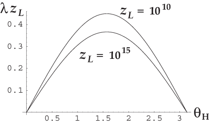
The first term in (23) dominates over the second. With given $z_{L}$, $c_{1}$ is fixed so as to reproduce the observed $m_{t}\sim 172\,$GeV at $\theta_{H}=\hbox{${1\over 2}$}\pi$. See Table I. With these parameters fixed, the $\theta_{H}$-dependence of $m_{t}$ is determined numerically, which is depicted in Fig. 1 for $z_{L}=10^{10}$ and $10^{15}$. The curves fit well with

with an error of $2.0\%\sim 4.0\%$. The top mass $m_{t}=\lambda k$ vanishes at $\theta_{H}=0$ as the chiral symmetry is restored. The effective potential $V_{\rm eff}(\theta_{H})$ is evaluated from the $\theta_{H}$-dependence of the mass spectrum. It was found that the contribution from the top quark dominates over those from gauge fields and other fermions. $V_{\rm eff}$ is minimized at $\theta_{H}=\pm\hbox{${1\over 2}$}\pi$.

To be definite, let us take $\mu_{j},\tilde{\mu}>0$ given by

which, a posteriori, leads to the value $m_{b}/m_{t}\sim 4.2/172$ for $c_{1}=c_{2}$. With the value $\lambda$ for the top quark, $\lambda S_{R}/[(\mu_{2}^{2}/2k)C_{L}]$ in the matrix $K$ in (S0.EGx4), for instance, is $O(10^{-15})$ so that the equation (S0.EGx4) is well approximated by

It follows that

The coefficient $a_{B+t}$ is determined so as to have canonical normalization for the kinetic term of $t_{L}(x)$. Note that $\lambda$ depends on $\theta_{H}$.

In the $Q_{\rm EM}=-\frac{1}{3}$ sector (the bottom sector) $b$, $D$, $X$, $b^{\prime}$, $\hat{D}_{R}$ and $\hat{X}_{R}$ mix with each other. As in the top sector, the bottom quark component $b(x)$ in four dimensions appears as

The brane fermions are related to the bulk fermions by

The equation corresponding to (S0.EGx4) is obtained by replacing $(U,B,t)$ by $(b,D,X)$ and interchanging $(c_{1},c_{2})$, $(\mu_{1},\mu_{3})$ and $(\mu_{2},\tilde{\mu})$. In the same approximation as in the top case the bottom mass and the coefficients $a_{j}$’s are found, for $0<c_{1},c_{2}<\hbox{${1\over 2}$}$, to be

and

With the wave functions of the top and bottom quarks at hand, one can evaluate their Yukawa couplings in two manners. In the Kaluza-Klein approach we insert the wave functions into the five-dimensional Lagrangian density ${\cal L}_{\rm bulk}^{\rm fermion}+{\cal L}^{\rm brane}_{\rm mass}$ and integrate over the fifth dimensional coordinate to obtain four-dimensional Lagrangian. The part $k^{-1}\sum_{j=1}^{2}\overline{\tilde{\Psi}}_{j}(\gamma\partial)_{d=4}\tilde{\Psi}_{j}$ gives the four-dimensional kinetic terms for the top and bottom quarks. The part with the covariant derivative in the fifth coordinate

generates both the masses and Yukawa couplings of the top and bottom quarks. The 4D Higgs field is contained in the gauge potential $A_{z}$. The vev $v$ of $\phi^{4}(x)$ in (2) is related to $\theta_{H}$ by (3) and its fluctuation around $v$ corresponds to the neutral Higgs field $H(x)$. Hence the relevant part of the gauge potential is expressed as

in the original gauge where

In the twisted gauge defined in (8), $\tilde{A}_{z}^{c}=\raise 0.68889pt\hbox{$\langle$}\lower 0.68889pt\hbox{}\tilde{A}_{z}\,\raise 0.68889pt\hbox{$\rangle$}\lower 0.68889pt\hbox{}$ vanishes, $\tilde{A}_{z}(x,z)$ being expanded as in (34) with $\hat{\theta}_{H}$ replaced by $H(x)/f_{H}$.

The Yukawa coupling originates from $g_{A}({\Psi}_{L}^{\dagger}A_{z}{\Psi}_{R}+{\Psi}_{R}^{\dagger}A_{z}{\Psi}_{L})$ or $g_{A}({\tilde{\Psi}}_{L}^{\dagger}\tilde{A}_{z}{\tilde{\Psi}}_{R}+{\tilde{\Psi}}_{R}^{\dagger}\tilde{A}_{z}{\tilde{\Psi}}_{L})$, whereas the mass term comes from $-i{\Psi}_{L}^{\dagger}\big(D_{-}+ig_{A}A_{z}^{c}\big){\Psi}_{R}+i{\Psi}_{R}^{\dagger}\big(D_{+}-ig_{A}A_{z}^{c}\big){\Psi}_{L}$ in the original gauge or $-i{\tilde{\Psi}}_{jL}^{\dagger}D_{-}{\tilde{\Psi}}_{jR}+i{\tilde{\Psi}}_{jR}^{\dagger}D_{+}{\tilde{\Psi}}_{jL}$ in the twisted gauge. The terms involving $D_{\pm}$ are important. With the wave function in (2), (13) and (29) inserted, $\varphi_{H}(z){\tilde{\Psi}}_{jL}^{\dagger}T^{\hat{4}}\tilde{\Psi}_{jR}$ ($\varphi_{H}(z){\tilde{\Psi}}_{jR}^{\dagger}T^{\hat{4}}\tilde{\Psi}_{jL}$) has different $z$-dependence from ${\tilde{\Psi}}_{jL}^{\dagger}D_{-}\tilde{\Psi}_{jR}$ (${\tilde{\Psi}}_{jR}^{\dagger}D_{+}\tilde{\Psi}_{jL}$). After the integration over $z$, the Yukawa coupling is not proportional to the fermion mass in the RS spacetime. We also recall that a large gauge transformation generates $\theta_{H}\rightarrow\theta_{H}+2\pi$ so that the mass spectrum remains invariant under the shift $\theta_{H}\rightarrow\theta_{H}+2\pi$, or equivalently under $H(x)\rightarrow H(x)+2\pi f_{H}$. The mass is a periodic, nonlinear function of $\theta_{H}$. (There is no level-crossing in the RS spacetime.) The nonlinearity in the relation between the Yukawa coupling and mass is confirmed by direct evaluation described below.

Let us define the normalized coefficients $a^{\prime L,R}_{j}$ by

where $N_{C_{L}}^{(j)}=\int_{1}^{z_{L}}dz\,C_{L}(z;\lambda,c_{j})^{2}$ etc.. Then the free part of the Lagrangian for the top quark is found to be

The contributions coming from the brane mass term ${\cal L}^{\rm brane}_{\rm mass}$ turn out $O(10^{-15})$ smaller than $P_{L}$ and $P_{R}$, and can be ignored.

Recall that $D_{-}S_{R}=\lambda C_{L}$ and $D_{+}C_{L}=\lambda S_{R}$, from which it follows that $N_{C_{L}}=N_{S_{R}}+\lambda^{-1}S_{R}C_{L}|_{z=1}$. Hence

The relations (27) and $C_{L}C_{R}-S_{L}S_{R}=1$ have been used in the second equality. The last equality follows from the relation (23) determining the mass spectrum. Let us adopt the normalization $P_{L}=P_{R}=1$ with which the top mass appears as $\lambda k$ in (39) as it should. The coefficients $a^{\prime L}_{j}$ and $a^{\prime R}_{j}$ represent how much portion of each field contains the left- and right-handed top quark, respectively.

Similarly the normalized coefficients $a^{\prime L,R}_{b}$, $a^{\prime L,R}_{D\pm X}$, $a^{\prime L,R}_{b^{\prime}}$ are determined. The numerical values are tabulated in Table II. The numerical values for the dominant terms ($a^{\prime L}_{B\pm t}$, $a^{\prime L,R}_{t^{\prime}}$, $a^{\prime L}_{b}$, $a^{\prime L}_{D\pm X}$, and $a^{\prime R}_{b^{\prime}}$) do not vary very much with $z_{L}$ in the range $10^{10}$ to $10^{15}$. In the $\theta_{H}=0$ limit, the four-dimensional $t_{L}(x)$ and $t_{R}(x)$ are mostly contained in the five-dimensional $t$ and $t^{\prime}$, respectively. At $\theta_{H}=\hbox{${1\over 2}$}\pi$, $t_{L}(x)$ resides in the $(B+t)/\sqrt{2}$ and $t^{\prime}$ components, whereas $t_{R}(x)$ remains in $t^{\prime}$. The four-dimensional $b_{L}(x)$ and $b_{R}(x)$ are mostly contained, for any value of $\theta_{H}$, in the five-dimensional $b$ and $b^{\prime}$, respectively.