跳到论文正文
W Papers独立论文阅读器 arXiv:0812.4589 论文正文 计算阅读时间 · 0%
引用这篇论文根据当前论文元数据生成,正式投稿前建议核对。


License: arXiv.org perpetual non-exclusive license
arXiv:0812.4589v2 [math.GT] 15 Jun 2010

Pseudo-Anosov braids with small entropy and the magic 33-manifold

Eiko Kin Note: The author is partially supported by Grant-in-Aid for Young Scientists (B) (No. 20740031), MEXT, Japan    and Mitsuhiko Takasawa
Abstract

We consider a surface bundle over the circle, the so called magic manifold MM. We determine homology classes whose minimal representatives are genus 00 fiber surfaces for MM, and describe their monodromies by braids. Among those classes whose representatives have nn punctures for each nn, we decide which one realizes the minimal entropy. We show that for each n≥9n\geq 9 (resp. n=3,4,5,7,8n=3,4,5,7,8), there exists a pseudo-Anosov homeomorphism Φn:Dn→Dn\Phi_{n}:D_{n}\rightarrow D_{n} with the smallest known entropy (resp. the smallest entropy) which occurs as the monodromy on an nn-punctured disk fiber for the Dehn filling of MM. A pseudo-Anosov homeomorphism Φ6:D6→D6\Phi_{6}:D_{6}\rightarrow D_{6} with the smallest entropy occurs as the monodromy on a 66-punctured disk fiber for MM.

Keywords: mapping class group, pseudo-Anosov, entropy, hyperbolic volume, magic manifold

Mathematics Subject Classification : Primary 37E30, 57M27, Secondary 57M50

1 Introduction

Let ℳ⁡(Σ)\mathcal{M}(\Sigma) be the mapping class group of an orientable surface Σ=Σg,p\Sigma=\Sigma_{g,p} of genus gg with pp punctures. Assuming that 3​g−3+p≥13g-3+p\geq 1, elements of ℳ⁡(Σ)\mathcal{M}(\Sigma) are classified into three types: periodic, pseudo-Anosov and reducible [29]. There exist two numerical invariants of pseudo-Anosov mapping classes ϕ\phi. One is the entropy ent⁡(ϕ)\mathrm{ent}(\phi) which is the logarithm of the dilatation λ⁡(ϕ)\lambda(\phi). The other is the volume vol⁡(ϕ)\mathrm{vol}(\phi) which comes from the hyperbolization theorem by Thurston [30]. His theorem asserts that ϕ\phi is pseudo-Anosov if and only if its mapping torus

𝕋(ϕ)=Σ×[0,1]/∼,{\mathbb{T}}(\phi)=\Sigma\times[0,1]/\sim,

where ∼\sim identifies (x,1)(x,1) with (f⁡(x),0)(f(x),0) for any representative f∈ϕf\in\phi, is hyperbolic. We denote the volume of 𝕋⁡(ϕ){\mathbb{T}}(\phi) by vol⁡(ϕ)\mathrm{vol}(\phi).

Let ℳpA​(Σ)\mathcal{M}^{\mathrm{pA}}(\Sigma) be the set of pseudo-Anosov elements of ℳ⁡(Σ)\mathcal{M}(\Sigma). Fixing Σ\Sigma, the dilatation λ⁡(ϕ)\lambda(\phi) for ϕ∈ℳpA​(Σ)\phi\in\mathcal{M}^{\mathrm{pA}}(\Sigma) is known to be an algebraic integer with a bounded degree depending only on Σ\Sigma. The set of dilatations λ⁡(ϕ)\lambda(\phi) for ϕ∈ℳpA​(Σ)\phi\in\mathcal{M}^{\mathrm{pA}}(\Sigma) bounded by each constant from above is finite, see [13]. In particular the set

Dil⁡(Σ)={λ⁡(ϕ)>1|ϕ∈ℳpA​(Σ)}\mathrm{Dil}(\Sigma)=\{\lambda(\phi)>1\ |\ \phi\in\mathcal{M}^{\mathrm{pA}}(\Sigma)\}

achieves its infimum λ⁡(Σ)\lambda(\Sigma).

We turn to volume. The set

{v|v​is the volume of a hyperbolic ​3​-manifold}\{v\ |\ v\ \mbox{is\ the\ volume\ of\ a\ hyperbolic\ }3\mbox{-manifold}\}

is a well-ordered closed subset of ℝ{\mathbb{R}} of order type ωω\omega^{\omega} [27]. In particular any subset achieves its infimum. Let vol⁡(Σ)=min⁡{vol⁡(ϕ)|ϕ∈ℳpA​(Σ)}\mathrm{vol}(\Sigma)=\min\{\mathrm{vol}(\phi)\ |\ \phi\in\mathcal{M}^{\mathrm{pA}}(\Sigma)\}. It is of interest to compute λ⁡(Σ)\lambda(\Sigma) (resp. vol⁡(Σ)\mathrm{vol}(\Sigma)) and to determine the mapping class realizing the minimum. Another problem related to the minimal dilatation (resp. minimal volume) are as follows. For a non-negative integer cc, we set

λ⁡(Σ,c)\displaystyle\lambda(\Sigma;c) =\displaystyle= min{λ(ϕ)|ϕ∈ℳp​A(Σ),𝕋(ϕ)has c cusps},\displaystyle\min\{\lambda(\phi)\ |\ \phi\in\mathcal{M}^{\mathrm{p}A}(\Sigma),\ {\mathbb{T}}(\phi)\ \mbox{has\ }c\mbox{\ cusps}\},
vol⁡(Σ,c)\displaystyle\mathrm{vol}(\Sigma;c) =\displaystyle= min{vol(ϕ)|ϕ∈ℳpA(Σ),𝕋(ϕ)has c cusps}.\displaystyle\min\{\mathrm{vol}(\phi)\ |\ \phi\in\mathcal{M}^{\mathrm{pA}}(\Sigma),\ {\mathbb{T}}(\phi)\ \mbox{has\ }c\mbox{\ cusps}\}.

A problem is to compute λ⁡(Σ,c)\lambda(\Sigma;c) (resp. vol⁡(Σ,c)\mathrm{vol}(\Sigma;c)) and to find a mapping class realizing the minimum.

In [15], the authors and S. Kojima obtain experimental results concerning the entropy and volume. In the case the mapping class group ℳ⁡(Dn)\mathcal{M}(D_{n}) of an nn-punctured disk DnD_{n}, they observe that for many pairs (n,c)(n,c), there exists a mapping class simultaneously reaching both λ⁡(Dn,c)\lambda(D_{n};c) and vol⁡(Dn,c)\mathrm{vol}(D_{n};c). Experiments tell us that in case c=3c=3, the mapping tori reaching both minima are homeomorphic to the magic manifold MmagicM_{\mathrm{magic}} which is the exterior of the 33 chain link 𝒞3\mathcal{C}_{3} illustrated in Figure 1. Moreover when c=2c=2, it is observed that there exists a mapping class ϕ\phi realizing both λ⁡(Dn,2)\lambda(D_{n};2) and vol⁡(Dn,2)\mathrm{vol}(D_{n};2) and its mapping torus 𝕋⁡(ϕ){\mathbb{T}}(\phi) is homeomorphic to a Dehn filling of MmagicM_{\mathrm{magic}} along one cusp. This study motivates the present paper which concerns the fibrations in MmagicM_{\mathrm{magic}}. The magic manifold has the smallest known volume among orientable hyperbolic 33-manifolds having 33 cusps. Many manifolds having at most 22 cusps with small volume are obtained from MmagicM_{\mathrm{magic}} by Dehn fillings, see [21]. Also, some important examples for the study of the exceptional Dehn fillings can be obtained from the Dehn fillings of MmagicM_{\mathrm{magic}}, see [9].

Let MM be a hyperbolic 33-manifold with boundary which fibers over the circle. We assume that MM admits infinitely many different fibrations. Thurston introduced the norm function XT:H2​(M,∂M,ℝ)→ℝX_{T}:H_{2}(M,\partial M;{\mathbb{R}})\rightarrow{\mathbb{R}}, and showed that the unit ball UU with respect to XTX_{T} is a compact, convex polyhedron [28]. He described the relation between the function XTX_{T} and fibrations of MM as follows. For each fiber FF of MM, the homology class [F]∈H2​(M,∂M,ℝ)[F]\in H_{2}(M,\partial M;{\mathbb{R}}) lies in the open cone i​n​t​(CΔ)int(C_{\Delta}) with the origin over a top dimensional face Δ\Delta of ∂U\partial U. Conversely for any integral class a∈i​n​t​(CΔ)a\in int(C_{\Delta}), there exists a fiber FF of MM representing aa. Using this description of the fibers, the entropy function ent⁡(⋅):i​n​t​(CΔ)→ℝ\mathrm{ent}(\cdot):int(C_{\Delta})\rightarrow{\mathbb{R}} can be defined as follows. For each primitive integral class a∈i​n​t​(CΔ)a\in int(C_{\Delta}), the monodromy Φa:Fa→Fa\Phi_{a}:F_{a}\rightarrow F_{a} on a connected surface FaF_{a} representing aa is pseudo-Anosov, and one defines the entropy of aa by ent⁡(a)=log⁡(λ⁡(Φa))\mathrm{ent}(a)=\log(\lambda(\Phi_{a})). Fried proves that this function defined on primitive integral classes admits a unique continuous extension to a homogeneous function on i​n​t​(CΔ)int(C_{\Delta}) [6].

One sees that ℳ⁡(Dn)\mathcal{M}(D_{n}) is isomorphic to the subgroup of ℳ⁡(Σ0,n+1)\mathcal{M}(\Sigma_{0,n+1}) consisting of the elements which fix the puncture of Σ0,n+1\Sigma_{0,n+1}. By using the natural surjective homomorphism Γ:Bn→ℳ⁡(Dn)\Gamma:B_{n}\rightarrow\mathcal{M}(D_{n}) from the nn-braid group BnB_{n} to ℳ⁡(Dn)\mathcal{M}(D_{n}), one represents each element of ℳ⁡(Dn)\mathcal{M}(D_{n}) by an nn-braid. A braid bb is called pseudo-Anosov if Γ⁡(b)\Gamma(b) is a pseudo-Anosov mapping class. If this is the case, the dilatation λ⁡(b)\lambda(b) of bb is defined by the dilatation of Γ⁡(b)\Gamma(b). Let Tm,pT_{m,p} be the following mm-braid for m≥3m\geq 3 and p≥1p\geq 1 which is a main example in this paper.

Tm,p=(σ12σ2σ3⋯σm−1)pσm−1−2.T_{m,p}=(\sigma_{1}^{2}\sigma_{2}\sigma_{3}\cdots\sigma_{m-1})^{p}\sigma_{m-1}^{-2}.

For example, T6,2=(σ12​σ2​σ3​σ4​σ5)2​σ5−2=σ12​σ2​σ3​σ4​σ5​σ12​σ2​σ3​σ4​σ5−1T_{6,2}=(\sigma_{1}^{2}\sigma_{2}\sigma_{3}\sigma_{4}\sigma_{5})^{2}\sigma_{5}^{-2}=\sigma_{1}^{2}\sigma_{2}\sigma_{3}\sigma_{4}\sigma_{5}\sigma_{1}^{2}\sigma_{2}\sigma_{3}\sigma_{4}\sigma_{5}^{-1} (Figure 8(left)). The braid Tm,pT_{m,p} is a horseshoe braid if gcd⁡(p,m−1)=1\gcd(p,m-1)=1 and 1<p≤m−121<p\leq\frac{m-1}{2} (Proposition 4.14). If gcd⁡(m−1,p)=1\gcd(m-1,p)=1, then the mapping torus 𝕋⁡(Γ⁡(Tm,p)){\mathbb{T}}(\Gamma(T_{m,p})) is homeomorphic to MmagicM_{\mathrm{magic}} (Corollary 3.28). Otherwise Γ⁡(Tm,p)\Gamma(T_{m,p}) is reducible. We set

ℳmagicn={ϕ∈ℳ⁡(Σ0,n)|𝕋⁡(ϕ)​is homeomorphic to ​Mmagic}.\mathcal{M}_{\mathrm{magic}}^{n}=\{\phi\in\mathcal{M}(\Sigma_{0,n})\ |\ {\mathbb{T}}(\phi)\ \mbox{is\ homeomorphic\ to\ }M_{\mathrm{magic}}\}.

Let us define an integral polynomial

f(x,y,z)​(t)=tx+y−z−tx−ty−tx−z−ty−z+1.f_{(x,y,z)}(t)=t^{x+y-z}-t^{x}-t^{y}-t^{x-z}-t^{y-z}+1.

The following, our main theorem, states that for all nn but 66 and 88, the minimum among the dilatations of ϕ∈ℳmagicn\phi\in\mathcal{M}_{\mathrm{magic}}^{n} is realized by Γ⁡(Tn−1,p)\Gamma(T_{n-1,p}) for some p=p⁡(n)p=p(n) and it is computed as the largest real root of one of the polynomials f(x,y,z)​(t)f_{(x,y,z)}(t).

Theorem 1.1.

For each n≥4n\geq 4, the minimum among the dilatations of ϕ∈ℳmagicn\phi\in\mathcal{M}_{\mathrm{magic}}^{n} is realized by:

(1)

Γ⁡(T2​k,2)\Gamma(T_{2k,2}) in case n=2​k+1n=2k+1 for k≥2k\geq 2. The dilatation λ⁡(T2​k,2)\lambda(T_{2k,2}) equals the largest real root of

f(k−1,k,0)​(t)=t2​k−1−2​(tk−1+tk)+1.f_{(k-1,k,0)}(t)=t^{2k-1}-2(t^{k-1}+t^{k})+1.
(2-i)

Γ⁡(σ1​σ22​σ3​σ4)\Gamma(\sigma_{1}\sigma_{2}^{2}\sigma_{3}\sigma_{4}) in case n=6n=6. The dilatation λ⁡(σ1​σ22​σ3​σ4)≈2.08102\lambda(\sigma_{1}\sigma_{2}^{2}\sigma_{3}\sigma_{4})\approx 2.08102 equals the largest real root of

f(3,2,1)​(t)=t4−t3−2​t3−t+1.f_{(3,2,1)}(t)=t^{4}-t^{3}-2t^{3}-t+1.
(2-ii)

Γ⁡(T4​k+1,2​k−1)\Gamma(T_{4k+1,2k-1}) in case n=4​k+2n=4k+2 for k≥2k\geq 2. The dilatation λ⁡(T4​k+1,2​k−1)\lambda(T_{4k+1,2k-1}) equals the largest real root of

f(2​k+1,2​k−1,0)​(t)=t4​k−2​(t2​k−1+t2​k+1)+1.f_{(2k+1,2k-1,0)}(t)=t^{4k}-2(t^{2k-1}+t^{2k+1})+1.
(3a-i)

Γ⁡(T3,1)\Gamma(T_{3,1}) in case n=4n=4. The dilatation λ⁡(T3,1)≈3.73205\lambda(T_{3,1})\approx 3.73205 equals the largest real root of

f(1,1,0)​(t)=t2−4​t+1.f_{(1,1,0)}(t)=t^{2}-4t+1.
(3a-ii)

Γ⁡(T8​k+3,2​k+1)\Gamma(T_{8k+3,2k+1}) in case n=8​k+4n=8k+4 for k≥1k\geq 1. The dilatation λ⁡(T8​k+3,2​k+1)\lambda(T_{8k+3,2k+1}) equals the largest real root of

f(4​k−1,4​k+3,0)​(t)=t8​k+2−2​(t4​k−1+t4​k+3)+1.f_{(4k-1,4k+3,0)}(t)=t^{8k+2}-2(t^{4k-1}+t^{4k+3})+1.
(3b-i)

Γ⁡(b)\Gamma(b) in case n=8n=8, where

b=σ1−1​σ2−1​σ3−1​σ4−1​σ5−1​σ6−1​σ1−1​σ2−1​σ3−1​σ4−1​σ1−1​σ2−1​σ3−1∈B7.b=\sigma_{1}^{-1}\sigma_{2}^{-1}\sigma_{3}^{-1}\sigma_{4}^{-1}\sigma_{5}^{-1}\sigma_{6}^{-1}\sigma_{1}^{-1}\sigma_{2}^{-1}\sigma_{3}^{-1}\sigma_{4}^{-1}\sigma_{1}^{-1}\sigma_{2}^{-1}\sigma_{3}^{-1}\in B_{7}.

The dilatation λ⁡(b)≈1.72208\lambda(b)\approx 1.72208 equals the largest real root of

f(5,3,2)​(t)=t6−t5−2​t3−t+1.f_{(5,3,2)}(t)=t^{6}-t^{5}-2t^{3}-t+1.
(3b-ii)

Γ⁡(T8​k+7,2​k+1)\Gamma(T_{8k+7,2k+1}) in case n=8​(k+1)n=8(k+1) for k≥1k\geq 1. The dilatation λ⁡(T8​k+7,2​k+1)\lambda(T_{8k+7,2k+1}) equals the largest real root of

f(4​k+5,4​k+1,0)​(t)=t8​k+6−2​(t4​k+1+t4​k+5)+1.f_{(4k+5,4k+1,0)}(t)=t^{8k+6}-2(t^{4k+1}+t^{4k+5})+1.

Moreover the above mapping class realizing the minimal dilatation among elements of ℳmagicn\mathcal{M}_{\mathrm{magic}}^{n} is unique up to conjugacy.

Refer to caption
Figure 1: 33 chain link 𝒞3\mathcal{C}_{3}.

Forgetting the 1st strand of Tm,pT_{m,p}, one obtains the (m−1)(m-1)-braid, call it Tm,p′T^{\prime}_{m,p}. For example, T6,2′=σ1​σ2​σ3​σ4​σ1​σ2​σ3​σ4−1T_{6,2}^{\prime}=\sigma_{1}\sigma_{2}\sigma_{3}\sigma_{4}\sigma_{1}\sigma_{2}\sigma_{3}\sigma_{4}^{-1}. The families of braids {Tm,p′}\{T^{\prime}_{m,p}\} and {Tm,p}\{T_{m,p}\} contain examples of ℓ\ell strands (ℓ=3,4,⋯,8\ell=3,4,\cdots,8) with the smallest dilatation. (See Section 4.1.) Hironaka-Kin (resp. Venzke) found candidates with the smallest dilatation λ⁡(Dn)\lambda(D_{n}) for nn odd (resp. nn even), see [12] (resp. [31]). All the braids in Theorem 1.1(1)(2-ii)(3a-ii)(3b-ii) relate to those examples. The braid T2​k,2′T_{2k,2}^{\prime} (with odd strands) is conjugate to the braid σ(k)\sigma_{(k)} with the smallest known dilatation found by Hironaka-Kin. (See Theorem 1.1(1).) For the braid Tm,p′T^{\prime}_{m,p} (with even strands) obtained from Tm,pT_{m,p} in (2-ii), (3a-ii) or (3b-ii) of Theorem 1.1, the mapping class Γ⁡(Tm,p′)\Gamma(T^{\prime}_{m,p}) is conjugate to the one given by Venzke. (See Section 4.1.)

Work of Farb-Leininger-Margalit [4] together with a result in [12] implies that there exists a complete, noncompact, finite volume, hyperbolic 33-manifold M′M^{\prime} with the following property: there exist Dehn fillings of M′M^{\prime} giving an infinite sequence of fiberings over S1S^{1}, with fibers DniD_{n_{i}} having nin_{i} punctures with ni→∞n_{i}\to\infty, and with the monodromy Φi:Dni→Dni\Phi_{i}:D_{n_{i}}\rightarrow D_{n_{i}} so that λ⁡(Dni)=λ⁡(Φi)\lambda(D_{n_{i}})=\lambda(\Phi_{i}). The magic manifold is a potential example which could satisfy this property.

In [1, 11, 17], one can find pseudo-Anosovs on closed surfaces Σg\Sigma_{g} of genus gg with small dilatation which occur as monodromies on fibers for Dehn fillings of MmagicM_{\mathrm{magic}}. Using those pseudo-Anosovs, Hironaka [11], Aaber-Dunfield [1], and the authors [17] independently proved that

limg→∞supg​log⁡λ⁡(Σg)≤log⁡(3+52).\displaystyle\lim_{g\to\infty}\sup g\log\lambda(\Sigma_{g})\leq\log(\tfrac{3+\sqrt{5}}{2}).

This paper is organized as follows. Section 2 reviews basic facts. Section 3 contains the proof of Theorem 1.1. For the proof, we first compute the Teichmüler polynomial, introduced by McMullen [24], which determines the entropy function for MmagicM_{\mathrm{magic}} (Theorem 3.3). Then we find all the homology classes whose representatives are genus 00 fiber surfaces (Corollary 3.10). We study the asymptotic behaviors of the normalized entropy function ent¯​(⋅)=XT​(⋅)​ent​(⋅)\overline{\mathrm{ent}}(\cdot)=X_{T}(\cdot)\mathrm{ent}(\cdot) (Theorem 3.11). This tells us which class realizes the minimal dilatation among homology classes whose representatives are genus 00 fiber surfaces with nn punctures (Proposition 3.12). We finally describe the monodromies for these fiber surfaces by using braids (Propositions 3.29 and 3.32). In Section 4, we discuss pseudo-Anosov braids with small dilatation. We also find a relation between the horseshoe map and the braids Tm,pT_{m,p} (Proposition 4.14).

Acknowledgments: We would like to thank Shigeki Akiyama and Takuya Sakasai who showed us the proof of Proposition 3.8. We would like to thank Sadayoshi Kojima and Makoto Sakuma for a great deal of encouragement. We also would like to thank the referees for valuable comments and suggestions.

2 Notation and basic facts

2.1 Mapping class group

The mapping class group ℳ⁡(Σ)\mathcal{M}(\Sigma) is the group of isotopy classes of orientation preserving homeomorphisms of Σ\Sigma, where the group operation is induced by composition of homeomorphisms. An element of the mapping class group is called a mapping class.

A homeomorphism Φ:Σ→Σ\Phi:\Sigma\rightarrow\Sigma is pseudo-Anosov if there exists a constant λ=λ⁡(Φ)>1\lambda=\lambda(\Phi)>1 called the dilatation of Φ\Phi and there exists a pair of transverse measured foliations ℱs\mathcal{F}^{s} and ℱu\mathcal{F}^{u} such that

Φ⁡(ℱs)=1λ​ℱs​and​Φ​(ℱu)=λ​ℱu.\Phi(\mathcal{F}^{s})=\tfrac{1}{\lambda}\mathcal{F}^{s}\ \mbox{and}\ \Phi(\mathcal{F}^{u})=\lambda\mathcal{F}^{u}.

In this case the mapping class ϕ=[Φ]\phi=[\Phi] is called pseudo-Anosov. We define the dilatation of ϕ\phi, denoted by λ⁡(ϕ)\lambda(\phi), to be the dilatation of Φ\Phi.

The (topological) entropy ent⁡(f)\mathrm{ent}(f) is a measure of the complexity of a continuous self-map ff on a compact manifold, see [32]. For a pseudo-Anosov homeomorphism Φ:Σ→Σ\Phi:\Sigma\rightarrow\Sigma, the equality

ent⁡(Φ)=log⁡(λ⁡(Φ))\mathrm{ent}(\Phi)=\log(\lambda(\Phi))

holds and ent⁡(Φ)\mathrm{ent}(\Phi) attains the minimal entropy among all homeomorphisms which are isotopic to Φ\Phi, see [5, Exposé 10]. We denote by ent⁡(ϕ)\mathrm{ent}(\phi) this characteristic number. Using the Euler characteristic χ⁡(Σ)\chi(\Sigma), we define the normalized entropy and normalized dilatation of ϕ\phi by ent¯​(ϕ)=|χ⁡(Σ)|​ent​(ϕ)\overline{\mathrm{ent}}(\phi)=|\chi(\Sigma)|\mathrm{ent}(\phi) and λ¯​(ϕ)=|χ⁡(Σ)|​λ​(ϕ)\overline{\lambda}(\phi)=|\chi(\Sigma)|\lambda(\phi).

We recall the surjective homomorphism

Γ:Bn→ℳ⁡(Dn)\Gamma:B_{n}\rightarrow\mathcal{M}(D_{n})

which sends the Artin generator σi\sigma_{i} for i∈{1,⋯,n−1}i\in\{1,\cdots,n-1\} (see Figure 2(left)) to t^i\hat{t}_{i}, where t^i\hat{t}_{i} is the mapping class which represents the positive half twist about the arc from the iith puncture to the (i+1)(i+1)st puncture. The kernel of Γ\Gamma is the center of BnB_{n} which is generated by the full twist (σ1σ2⋯σn−1)n(\sigma_{1}\sigma_{2}\cdots\sigma_{n-1})^{n}. By replacing the boundary of DnD_{n} with the (n+1)(n+1)st puncture, the injective homomorphism from ℳ⁡(Dn)\mathcal{M}(D_{n}) to ℳ⁡(Σ0,n+1)\mathcal{M}(\Sigma_{0,n+1}) is induced. In the rest of the paper we regard an element of ℳ⁡(Dn)\mathcal{M}(D_{n}) as an element of ℳ⁡(Σ0,n+1)\mathcal{M}(\Sigma_{0,n+1}).

We say that a braid b∈Bnb\in B_{n} is pseudo-Anosov if Γ⁡(b)∈ℳ⁡(Dn)\Gamma(b)\in\mathcal{M}(D_{n}) is pseudo-Anosov. Is the case, vol⁡(Γ⁡(b))\mathrm{vol}(\Gamma(b)) equals the hyperbolic volume of the exterior of the link b¯\overline{b} in S3S^{3}, where b¯\overline{b} is a union of the closed braid of bb and the braid axis. Our convention of the orientation of b¯\overline{b} is given by Figure 2(right).

Refer to caption
Figure 2: (left) generator σi\sigma_{i}. (right) braid b→b\rightarrow braided link b¯\overline{b}.

2.2 Roots of polynomials

Let f⁡(t)f(t) be an integral polynomial of degree dd. The reciprocal of f⁡(t)f(t) is f∗​(t)=td​f​(1/t)f_{*}(t)=t^{d}f(1/t). We denote by λ⁡(f)\lambda(f), the maximal absolute value of the roots of f⁡(t)f(t).

Let R⁡(t)R(t) be a monic integral polynomial and let S⁡(t)S(t) be an integral polynomial. We set

Qn,±​(t)=tn​R​(t)±S⁡(t)Q_{n,\pm}(t)=t^{n}R(t)\pm S(t)

for each integer n≥1n\geq 1. In case S​(t)=R∗​(t)S(t)=R_{*}(t), we call Qn,±​(t)=tn​R​(t)±R∗​(t)Q_{n,\pm}(t)=t^{n}R(t)\pm R_{*}(t) the Salem-Boyd polynomial associated to R⁡(t)R(t).

Lemma 2.1.

Let Qn,±​(t)=tn​R​(t)±S⁡(t)Q_{n,\pm}(t)=t^{n}R(t)\pm S(t). Suppose that R⁡(t)R(t) has a root outside the unit circle. Then, the roots of Qn,±​(t)Q_{n,\pm}(t) outside the unit circle converge to those of R⁡(t)R(t) counting multiplicity as nn goes to ∞\infty. In particular,

λ⁡(R)=limn→∞λ⁡(Qn,±).\lambda(R)=\lim_{n\to\infty}\lambda(Q_{n,\pm}).

The proof of Lemma 2.1 can be found in [16, Lemma 2.5].

2.3 Hyperbolic surface bundle over the circle

Let MM be an irreducible, atoroidal and oriented 33-manifold with boundary ∂M\partial M (possibly ∂M=∅\partial M=\emptyset). Thurston discovered a norm function XT:H2​(M,∂M,ℝ)→ℝX_{T}:H_{2}(M,\partial M;{\mathbb{R}})\rightarrow{\mathbb{R}} (see [28]). In case MM is a surface bundle over the circle, he described a relation between XTX_{T} and fibrations of MM which we record as Theorem 2.2 below.

2.3.1 Thurston norm

The norm function XT:H2​(M,∂M,ℝ)→ℝX_{T}:H_{2}(M,\partial M;{\mathbb{R}})\rightarrow{\mathbb{R}} has the property that for any integral class a∈H2​(M,∂M,ℝ)a\in H_{2}(M,\partial M;{\mathbb{R}}),

XT​(a)=minF⁡{−χ⁡(F)},X_{T}(a)=\min_{F}\{-\chi(F)\},

where the minimum is taken over all oriented surface FF embedded in MM, satisfying a=[F]a=[F], with no components of non-negative Euler characteristic. The surface FF which realizes this minimum is called a minimal representative of aa. For a rational class a∈H2​(M,∂M,ℝ)a\in H_{2}(M,\partial M;{\mathbb{R}}), take a rational number rr so that r​ara is an integral class. Then XT​(a)X_{T}(a) is defined to be

XT​(a)=1|r|​XT​(r​a).X_{T}(a)=\tfrac{1}{|r|}X_{T}(ra).

The function XTX_{T} defined on rational classes admits a unique continuous extension to H2​(M,∂M,ℝ)H_{2}(M,\partial M;{\mathbb{R}}) which is linear on the ray though the origin. The unit ball U={a∈H2​(M,∂M,ℝ)|XT​(a)≤1}U=\{a\in H_{2}(M,\partial M;{\mathbb{R}})\ |\ X_{T}(a)\leq 1\} is a compact, convex polyhedron [28].

The following notations are needed to describe how fibrations of MM are related to the Thurston norm.

  • •

    A top dimensional face in the boundary ∂U\partial U of the unit ball UU is denoted by Δ\Delta, and its open face is denoted by i​n​t​(Δ)int(\Delta).

  • •

    The open cone with the origin over Δ\Delta is denoted by i​n​t​(CΔ)int(C_{\Delta}).

  • •

    The set of integral classes of i​n​t​(CΔ)int(C_{\Delta}) is denoted by i​n​t​(CΔ​(ℤ))int(C_{\Delta}(\mathbb{Z})), and the set of rational classes of i​n​t​(CΔ)int(C_{\Delta}) is denoted by i​n​t​(CΔ​(ℚ))int(C_{\Delta}(\mathbb{Q})).

Theorem 2.2 ([28]).

Suppose that MM is a surface bundle over the circle and let FF be a fiber. Then there exists a top dimensional face Δ\Delta satisfying the following.

(1)

[F]∈i​n​t​(CΔ​(ℤ))[F]\in int(C_{\Delta}(\mathbb{Z})).

(2)

For any a∈i​n​t​(CΔ​(ℤ))a\in int(C_{\Delta}(\mathbb{Z})), a minimal representative EE of aa is a fiber of fibrations of MM.

The face Δ\Delta in Theorem 2.2 is called the fiber face. For the fiber face Δ\Delta, it follows that a∈i​n​t​(CΔ​(ℤ))a\in int(C_{\Delta}(\mathbb{Z})) is a primitive integral class if and only if a minimal representative EE of aa is connected.

It is known that if a0∈H2​(M,∂M,ℤ)a_{0}\in H_{2}(M,\partial M;{\mathbb{Z}}) has a representative FF which is a fiber of the fibration of MM, then any incompressible surface which represents a0a_{0} is isotopic to the fiber FF, see [28]. In particular FF is a minimal representative of a0a_{0}. Thus a minimal representative of a0a_{0} is unique up to isotopy.

2.3.2 Entropy function

Suppose that MM is a hyperbolic surface bundle over the circle. We fix a fiber face Δ\Delta for MM. The entropy function ent⁡(⋅):i​n​t​(CΔ​(ℚ))→ℝ\mathrm{ent}(\cdot):int(C_{\Delta}({\mathbb{Q}}))\rightarrow{\mathbb{R}} introduced by Fried in [6] is defined as follows. The minimal representative FaF_{a} for a∈i​n​t​(CΔ​(ℤ))a\in int(C_{\Delta}({\mathbb{Z}})) is a fiber of fibrations of MM. Let Φa:Fa→Fa\Phi_{a}:F_{a}\rightarrow F_{a} be the monodromy. Since MM is a hyperbolic manifold, the mapping class ϕa=[Φa]\phi_{a}=[\Phi_{a}] must be pseudo-Anosov. The entropy ent⁡(a)\mathrm{ent}(a) and dilatation λ⁡(a)\lambda(a) are defined as the entropy and dilatation of ϕa\phi_{a}, respectively. For a rational number rr and an integral class aa, the entropy ent⁡(r​a)\mathrm{ent}(ra) is defined by 1|r|​ent​(a).\frac{1}{|r|}\mathrm{ent}(a). Notice that XT​(⋅)​ent​(⋅):i​n​t​(CΔ​(ℚ))→ℝX_{T}(\cdot)\mathrm{ent}(\cdot):int(C_{\Delta}({\mathbb{Q}}))\rightarrow{\mathbb{R}} is constant on each ray through the origin. We call XT​(a)​ent​(a)X_{T}(a)\mathrm{ent}(a) and XT​(a)​λ​(a)X_{T}(a)\lambda(a) the normalized entropy and normalized dilatation of aa.

We recall an important property of the entropy function proved by Matsumoto and independently McMullen.

Theorem 2.3 ([22, 24]).

The function 1ent⁡(⋅):i​n​t​(CΔ​(ℚ))→ℝ\tfrac{1}{\mathrm{ent}(\cdot)}:int(C_{\Delta}({\mathbb{Q}}))\rightarrow{\mathbb{R}} is strictly concave.

By Theorem 2.3, the function ent⁡(⋅)\mathrm{ent}(\cdot) on i​n​t​(CΔ​(ℚ))int(C_{\Delta}({\mathbb{Q}})) admits a unique continuous extension to ent⁡(⋅):i​n​t​(CΔ)→ℝ\mathrm{ent}(\cdot):int(C_{\Delta})\rightarrow{\mathbb{R}}.

Since ent⁡(a)\mathrm{ent}(a) goes to ∞\infty as aa goes to a point on the boundary ∂Δ\partial\Delta (see [6]), Theorem 2.3 implies the normalized entropy function

ent¯​(⋅)=XT​(⋅)​ent​(⋅):i​n​t​(CΔ)→ℝ\overline{\mathrm{ent}}(\cdot)=X_{T}(\cdot)\mathrm{ent}(\cdot):int(C_{\Delta})\rightarrow{\mathbb{R}}

has the minimum at a unique ray through the origin. In other words ent⁡(⋅)\mathrm{ent}(\cdot) has the minimum at a unique point of i​n​t​(Δ)int(\Delta). The following question was posed by McMullen [24, p 542].

Problem 2.4.

On which ray does it attain the minimal normalized entropy with respect to the fiber face? Is the minimum always attained at a rational class of i​n​t​(Δ)int(\Delta)?

We solve this problem for the magic manifold in Section 3.2.

3 Magic manifold

3.1 Fiber face

Let 𝙻\mathtt{L} be one of the four lines in S3S^{3} depicted in Figure 3(1),(2),(3) and (4). For each 𝙻\mathtt{L}, there exist an integer nn and a periodic map f:(S3,𝒞3)→(S3,𝒞3)f:(S^{3},{\mathcal{C}}_{3})\rightarrow(S^{3},{\mathcal{C}}_{3}) such that ff is a 2​π/n2\pi/n rotation with respect to 𝙻\mathtt{L}. Such symmetry of 𝒞3{\mathcal{C}}_{3} reflects the shape of the Thurston unit ball. Let KαK_{\alpha}, KβK_{\beta} and KγK_{\gamma} be the components of 𝒞3\mathcal{C}_{3} such that KαK_{\alpha} (resp. KβK_{\beta}, KγK_{\gamma}) bounds the oriented twice-punctured disk FαF_{\alpha} (resp. FβF_{\beta}, FγF_{\gamma}) in MmagicM_{\mathrm{magic}} whose normal direction is indicated as in Figure 4(right). Those oriented surfaces induce the orientation of 𝒞3\mathcal{C}_{3}. Let α=[Fα]\alpha=[F_{\alpha}], β=[Fβ]\beta=[F_{\beta}], and γ=[Fγ]\gamma=[F_{\gamma}]. In [28], Thurston computes the unit ball UU which is the the parallelepiped with vertices ±α=(±1,0,0)\pm\alpha=(\pm 1,0,0), ±β=(0,±1,0)\pm\beta=(0,\pm 1,0), ±γ=(0,0,±1)\pm\gamma=(0,0,\pm 1), ±(α+β+γ)\pm(\alpha+\beta+\gamma), see Figure 4(left). The set {α,β,γ}\{\alpha,\beta,\gamma\} is a basis of H2​(Mmagic,∂Mmagic,ℤ)H_{2}(M_{\mathrm{magic}},\partial M_{\mathrm{magic}};{\mathbb{Z}}).

Refer to caption
Figure 3: axis 𝙻\mathtt{L} for periodic map
Refer to caption
Figure 4: (left) Thurston unit ball. (right) FαF_{\alpha}, FβF_{\beta}, FγF_{\gamma}. (arrows indicate the normal direction of oriented surfaces.)

The magic manifold is a surface bundle over the circle as we will see it later. The symmetry of 𝒞3{\mathcal{C}}_{3} tells us that every top dimensional face is a fiber face. We (arbitrarily) pick the shaded fiber face Δ\Delta as in Figure 5(left) with vertices α=(1,0,0)\alpha=(1,0,0), α+β+γ=(1,1,1)\alpha+\beta+\gamma=(1,1,1), β=(0,1,0)\beta=(0,1,0) and −γ=(0,0,−1)-\gamma=(0,0,-1). The open face i​n​t​(Δ)int(\Delta) is written by

int(Δ)={xα+yβ+zγ|x+y−z=1,x>0,y>0,x>z,y>z}.int(\Delta)=\{x\alpha+y\beta+z\gamma\ |\ x+y-z=1,\ x>0,\ y>0,\ x>z,\ y>z\}. (3.1)

For x​α+y​β+z​γ∈i​n​t​(CΔ)x\alpha+y\beta+z\gamma\in int(C_{\Delta}) (not necessarily primitive),

XT​(x​α+y​β+z​γ)=x+y−z.X_{T}(x\alpha+y\beta+z\gamma)=x+y-z.
Refer to caption
Figure 5: (left) fiber face Δ\Delta. (center) Δ1⊂Δ\Delta_{1}\subset\Delta. (right) CΔ1⊂i​n​t​(CΔ)C_{\Delta_{1}}\subset int(C_{\Delta}).

Let 𝒩⁡(L)\mathcal{N}(L) be the regular neighborhood of a link LL in S3S^{3}. We denote the tori ∂𝒩⁡(Kα)\partial\mathcal{N}(K_{\alpha}), ∂𝒩⁡(Kβ)\partial\mathcal{N}(K_{\beta}), ∂𝒩⁡(Kγ)\partial\mathcal{N}(K_{\gamma}) by TαT_{\alpha}, TβT_{\beta}, TγT_{\gamma} respectively. Let x​α+y​β+z​γx\alpha+y\beta+z\gamma be a primitive integral class in i​n​t​(CΔ)int(C_{\Delta}). We denote by Fx​α+y​β+z​γF_{x\alpha+y\beta+z\gamma} or F(x,y,z)F_{(x,y,z)}, the minimal representative of x​α+y​β+z​γx\alpha+y\beta+z\gamma. Let us set

∂αF(x,y,z)=∂F(x,y,z)∩Tα\partial_{\alpha}F_{(x,y,z)}=\partial F_{(x,y,z)}\cap T_{\alpha}

which consists of the parallel simple closed curves on TαT_{\alpha}. We define the subsets ∂βF(x,y,z)\partial_{\beta}F_{(x,y,z)}, ∂γF(x,y,z)⊂∂F(x,y,z)\partial_{\gamma}F_{(x,y,z)}\subset\partial F_{(x,y,z)} in the same manner. We denote by Φ(x,y,z):F(x,y,z)→F(x,y,z)\Phi_{(x,y,z)}:F_{(x,y,z)}\rightarrow F_{(x,y,z)}, the monodromy on a fiber F(x,y,z)F_{(x,y,z)}. It is clear that Φ(x,y,z)\Phi_{(x,y,z)} permutes elements of each of the sets ∂αF(x,y,z)\partial_{\alpha}F_{(x,y,z)}, ∂βF(x,y,z)\partial_{\beta}F_{(x,y,z)} and ∂γF(x,y,z)\partial_{\gamma}F_{(x,y,z)} cyclically. Let ℱ(x,y,z)\mathcal{F}_{(x,y,z)} be the stable foliation for the pseudo-Anosov Φ(x,y,z)\Phi_{(x,y,z)}.

Lemma 3.1.

Let x​α+y​β+z​γ∈i​n​t​(CΔ)x\alpha+y\beta+z\gamma\in int(C_{\Delta}) be a primitive integral class. The number of the boundary components ♯⁡(∂F(x,y,z))\sharp(\partial F_{(x,y,z)}) is equal to the sum of the three greatest common divisors

gcd⁡(x,y+z)+gcd⁡(y,z+x)+gcd⁡(z,x+y),\gcd(x,y+z)+\gcd(y,z+x)+\gcd(z,x+y),

where gcd⁡(0,w)\gcd(0,w) is defined by |w||w|. More precisely

(1)

♯⁡(∂αF(x,y,z))=gcd⁡(x,y+z)\sharp(\partial_{\alpha}F_{(x,y,z)})=\gcd(x,y+z),

(2)

♯⁡(∂βF(x,y,z))=gcd⁡(y,z+x)\sharp(\partial_{\beta}F_{(x,y,z)})=\gcd(y,z+x),

(3)

♯⁡(∂γF(x,y,z))=gcd⁡(z,x+y)\sharp(\partial_{\gamma}F_{(x,y,z)})=\gcd(z,x+y).

Proof. We prove (1). The proof of (2),(3) is similar. We have the meridian and longitude basis {mα,ℓα}\{m_{\alpha},\ell_{\alpha}\} for TαT_{\alpha}. Similarly we have the bases {mβ,ℓβ}\{m_{\beta},\ell_{\beta}\} for TβT_{\beta} and {mγ,ℓγ}\{m_{\gamma},\ell_{\gamma}\} for TγT_{\gamma}. We consider the long exact sequence of the homology groups of the pair (Mmagic,∂Mmagic)(M_{\mathrm{magic}},\partial M_{\mathrm{magic}}). The boundary map is given by

∂∗:H2​(Mmagic,∂Mmagic,ℝ)\displaystyle\partial_{*}:H_{2}(M_{\mathrm{magic}},\partial M_{\mathrm{magic}};{\mathbb{R}}) →\displaystyle\rightarrow H1​(∂Mmagic,ℝ),\displaystyle H_{1}(\partial M_{\mathrm{magic}};{\mathbb{R}}),
α\displaystyle\alpha ↦\displaystyle\mapsto ℓα−mβ−mγ,\displaystyle\ell_{\alpha}-m_{\beta}-m_{\gamma},
β\displaystyle\beta ↦\displaystyle\mapsto ℓβ−mγ−mα,\displaystyle\ell_{\beta}-m_{\gamma}-m_{\alpha},
γ\displaystyle\gamma ↦\displaystyle\mapsto ℓγ−mα−mβ.\displaystyle\ell_{\gamma}-m_{\alpha}-m_{\beta}.

Hence

∂∗(x​α+y​β+z​γ)=x​ℓα−(y+z)​mα+y​ℓβ−(z+x)​mβ+z​ℓγ−(x+y)​mγ.\partial_{*}(x\alpha+y\beta+z\gamma)=x\ell_{\alpha}-(y+z)m_{\alpha}+y\ell_{\beta}-(z+x)m_{\beta}+z\ell_{\gamma}-(x+y)m_{\gamma}. (3.2)

Since F(x,y,z)F_{(x,y,z)} is the minimal representative, the set ∂αF(x,y,z)\partial_{\alpha}F_{(x,y,z)} is a union of oriented parallel simple closed curves on TαT_{\alpha} whose homology class equals x​ℓα−(y+z)​mα∈H1​(Tα,ℝ)x\ell_{\alpha}-(y+z)m_{\alpha}\in H_{1}(T_{\alpha};{\mathbb{R}}), see (3.2). Thus the number of the components of ∂αF(x,y,z)\partial_{\alpha}F_{(x,y,z)} equals gcd⁡(x,y+z)\gcd(x,y+z). □\Box

In Section 4.1, we will use the following to see λ⁡(Tm,p′)\lambda(T_{m,p}^{\prime}) is equal to λ⁡(Tm,p)\lambda(T_{m,p}).

Lemma 3.2 ([17]).

Let x​α+y​β+z​γx\alpha+y\beta+z\gamma be as in Lemma 3.1. The stable foliation ℱ(x,y,z)\mathcal{F}_{(x,y,z)} has

(1)

xgcd⁡(x,y+z)\tfrac{x}{\gcd(x,y+z)} prongs at each element of ∂αF(x,y,z)\partial_{\alpha}F_{(x,y,z)},

(2)

ygcd⁡(y,x+z)\tfrac{y}{\gcd(y,x+z)} prongs at each element of ∂βF(x,y,z)\partial_{\beta}F_{(x,y,z)},

(3)

x+y−2​zgcd⁡(z,x+y)\tfrac{x+y-2z}{\gcd(z,x+y)} prongs at each element of ∂γF(x,y,z)\partial_{\gamma}F_{(x,y,z)}, and

(4)

no singularities in the interior of F(x,y,z)F_{(x,y,z)}.

3.2 Teichmüler polynomial

We compute the Teichmüler polynomial P=PΔP=P_{\Delta} with respect to Δ\Delta. For background, see [24].

A fiber F=F(1,1,0)F=F_{(1,1,0)} is homeomorphic to a sphere with 44 boundary components. We now see that the monodromy Φ=Φ(1,1,0)\Phi=\Phi_{(1,1,0)} on FF is represented by the 33-braid b=σ2​σ1−1​σ2b=\sigma_{2}\sigma_{1}^{-1}\sigma_{2}. A homeomorphism H:S3∖𝒩⁡(𝒞3)→S3∖𝒩⁡(b¯)H:S^{3}\setminus\mathcal{N}(\mathcal{C}_{3})\rightarrow S^{3}\setminus\mathcal{N}(\overline{b}) is given as follows. The link illustrated in Figure 6(left) is isotopic to 𝒞3\mathcal{C}_{3}. We consider the exterior S3∖𝒞3S^{3}\setminus\mathcal{C}_{3} and we open the twice-punctured disk FαF_{\alpha} bounded by KαK_{\alpha}. Let Fα′F^{\prime}_{\alpha} and Fα′′F^{\prime\prime}_{\alpha} be the resulting twice-punctured disks obtained from FαF_{\alpha}. Reglue Fα′F^{\prime}_{\alpha} and Fα′′F^{\prime\prime}_{\alpha} by twisting one of the disks by 360360 degrees in the clockwise direction. Then we obtain the braided link b¯\overline{b} whose exterior S3∖b¯S^{3}\setminus\overline{b} is homeomorphic to S3∖𝒞3S^{3}\setminus\mathcal{C}_{3}, see Figure 6.

Refer to caption
Figure 6: (left) 𝒞3\mathcal{C}_{3}. (right) b¯\overline{b}. (this figure explains how to obtain HH.)

Let uu be the meridian of the component of b¯\overline{b} which is the braid axis. Let t2t_{2} (resp. t1t_{1}) be the meridian of the component of b¯\overline{b} which is the closure of the second strand of bb (resp. which is the closure of the rest of the strand of bb). By using the argument in [24, Section 11], one sees that the Teichmüler polynomial P⁡(t1,t2,u)P(t_{1},t_{2},u) is given by

P⁡(t1,t2,u)=det(u​I−σ2−1​(t2)​σ1​(t1)​σ2−1​(t1)),P(t_{1},t_{2},u)=\det(uI-\sigma_{2}^{-1}(t_{2})\sigma_{1}(t_{1})\sigma_{2}^{-1}(t_{1})),

where σ1​(t)=(tt01)\sigma_{1}(t)=\left(\begin{array}[]{cc}t&t\\ 0&1\end{array}\right) and σ2−1​(t)=(10t−1t−1)\sigma_{2}^{-1}(t)=\left(\begin{array}[]{cc}1&0\\ t^{-1}&t^{-1}\end{array}\right). (Note that our convention of the sign of braids is different from the one in [24].) Hence

P⁡(t1,t2,u)=1t2−u−t1​u−ut2−ut1​t2+u2.P(t_{1},t_{2},u)=\tfrac{1}{t_{2}}-u-t_{1}u-\tfrac{u}{t_{2}}-\tfrac{u}{t_{1}t_{2}}+u^{2}.

Now we transform this to the polynomial using our basis. Let {α∗,β∗,γ∗}\{\alpha^{*},\beta^{*},\gamma^{*}\} be the dual basis for H1​(Mmagic,ℤ)H_{1}(M_{\mathrm{magic}};{\mathbb{Z}}). We set s1=α∗s_{1}=\alpha^{*}, s2=β∗s_{2}=\beta^{*}, s3=γ∗s_{3}=\gamma^{*}. By the construction of the homeomorphism HH, one observes that t1=s3t_{1}=s_{3}, t2=s1​s2−1​s3−1t_{2}=s_{1}s_{2}^{-1}s_{3}^{-1} and u=s2u=s_{2}. We obtain

P⁡(s1,s2,s3)=−s1−s2+s3+s1​s2−s1​s3−s2​s3.P(s_{1},s_{2},s_{3})=-s_{1}-s_{2}+s_{3}+s_{1}s_{2}-s_{1}s_{3}-s_{2}s_{3}.
Theorem 3.3.

The dilatation of x​α+y​β+z​γ∈i​n​t​(CΔ​(ℤ))x\alpha+y\beta+z\gamma\in int(C_{\Delta}(\mathbb{Z})) is the largest real root of

P⁡(s1=tx,s2=ty,s3=tz)=−tx−ty+tz+tx+y−tx+z−ty+z.P(s_{1}=t^{x},s_{2}=t^{y},s_{3}=t^{z})=-t^{x}-t^{y}+t^{z}+t^{x+y}-t^{x+z}-t^{y+z}.

In particular, the dilatation of x​α+y​β∈i​n​t​(CΔ​(ℤ))x\alpha+y\beta\in int(C_{\Delta}(\mathbb{Z})) is the largest real root of tx+y−2​(tx+ty)+1.t^{x+y}-2(t^{x}+t^{y})+1.

Proof. We identify H2​(Mmagic,∂Mmagic)H_{2}(M_{\mathrm{magic}},\partial M_{\mathrm{magic}}) with H1​(Mmagic,∂Mmagic)H^{1}(M_{\mathrm{magic}},\partial M_{\mathrm{magic}}). By [24, Section 1], the dilatation of a=x​α+y​β+z​γa=x\alpha+y\beta+z\gamma is equal to the largest real root of

P⁡(s1=ta⁡(α∗),s2=ta⁡(β∗),s3=ta⁡(γ∗))=P⁡(tx,ty,tz)\displaystyle P(s_{1}=t^{a(\alpha^{*})},s_{2}=t^{a(\beta^{*})},s_{3}=t^{a(\gamma^{*})})=P(t^{x},t^{y},t^{z})
=\displaystyle= −tx−ty+tz+tx+y−tx+z−ty+z.\displaystyle-t^{x}-t^{y}+t^{z}+t^{x+y}-t^{x+z}-t^{y+z}.

This completes the proof. □\Box

Since

P⁡(tx,ty,tz)=tz​(tx+y−z−tx−ty−tx−z−ty−z+1),P(t^{x},t^{y},t^{z})=t^{z}(t^{x+y-z}-t^{x}-t^{y}-t^{x-z}-t^{y-z}+1),

the dilatation of x​α+y​β+z​γx\alpha+y\beta+z\gamma is the largest real root of

f(x,y,z)​(t)=tx+y−z−tx−ty−tx−z−ty−z+1.f_{(x,y,z)}(t)=t^{x+y-z}-t^{x}-t^{y}-t^{x-z}-t^{y-z}+1.
Remark 3.4.

Oertel obtained similar polynomial with respect to each fiber face as the Teichmüler polynomial, see [25].

Remark 3.5.

For x≥y>0x\geq y>0 and z>0z>0,

f(x,y,−z)​(t)=f(x+z,y+z,z)​(t)=tx+y+z−tx+z−ty+z−tx−ty+1.f_{(x,y,-z)}(t)=f_{(x+z,y+z,z)}(t)=t^{x+y+z}-t^{x+z}-t^{y+z}-t^{x}-t^{y}+1.

Thus,

λ⁡(x​α+y​β−z​γ)=λ⁡((x+z)​α+(y+z)​β+z​γ).\lambda(x\alpha+y\beta-z\gamma)=\lambda((x+z)\alpha+(y+z)\beta+z\gamma).
Theorem 3.6.

The homology class α+β\alpha+\beta realizes the minimal normalized entropy with respect to Δ\Delta, i.e, the ray through α+β\alpha+\beta attains the minimum of ent¯​(⋅)=XT​(⋅)​ent​(⋅):i​n​t​(CΔ)→ℝ\overline{\mathrm{ent}}(\cdot)=X_{T}(\cdot)\mathrm{ent}(\cdot):int(C_{\Delta})\rightarrow{\mathbb{R}}.

Proof. Clearly x​α+y​β+z​γx\alpha+y\beta+z\gamma is in i​n​t​(CΔ)int(C_{\Delta}) if and only if y​α+x​β+z​γy\alpha+x\beta+z\gamma is in i​n​t​(CΔ)int(C_{\Delta}). The equality ent¯​(x​α+y​β+z​γ)=ent¯​(y​α+x​β+z​γ)\overline{\mathrm{ent}}(x\alpha+y\beta+z\gamma)=\overline{\mathrm{ent}}(y\alpha+x\beta+z\gamma) holds, since these classes have the same entropy and the same Thurston norm. Thus if the minimum of ent¯\overline{\mathrm{ent}} is realized by the ray though x​α+y​β+z​γx\alpha+y\beta+z\gamma, then xx must equal yy.

On the other hand, x​α+x​β+γx\alpha+x\beta+\gamma and (x−1)​α+(x−1)​β−γ(x-1)\alpha+(x-1)\beta-\gamma have the same Thurston norm 2​x−12x-1 if x>1x>1. By Remark 3.5, they have the same entropy. Thus,

ent¯​(x​α+x​β+γ)=ent¯​((x−1)​α+(x−1)​β−γ).\overline{\mathrm{ent}}(x\alpha+x\beta+\gamma)=\overline{\mathrm{ent}}((x-1)\alpha+(x-1)\beta-\gamma).

Since ent¯\overline{\mathrm{ent}} is constant on each ray, we have

ent¯​(x​α+x​β+γ)\displaystyle\overline{\mathrm{ent}}(x\alpha+x\beta+\gamma) =\displaystyle= ent¯​(α+β+x−1​γ),\displaystyle\overline{\mathrm{ent}}(\alpha+\beta+x^{-1}\gamma),
ent¯​((x−1)​α+(x−1)​β−γ)\displaystyle\overline{\mathrm{ent}}((x-1)\alpha+(x-1)\beta-\gamma) =\displaystyle= ent¯​(α+β−(x−1)−1​γ).\displaystyle\overline{\mathrm{ent}}(\alpha+\beta-(x-1)^{-1}\gamma).

The minimal ray does not pass through both α+β+x−1​γ\alpha+\beta+x^{-1}\gamma and α+β−(x−1)−1​γ\alpha+\beta-(x-1)^{-1}\gamma, because the minimum is realized by a unique ray. Since x(>1)x(>1) is arbitrary, the desired ray must pass through α+β\alpha+\beta. □\Box

3.3 Fiber surface of genus 00

Let x​α+y​β+z​γ​i​n​t​(CΔ)x\alpha+y\beta+z\gamma int(C_{\Delta}) be an integral homology class. Recall that F(x,y,z)F_{(x,y,z)} is connected if and only if x​α+y​β+z​γx\alpha+y\beta+z\gamma is primitive. Since {α,β,γ}\{\alpha,\beta,\gamma\} is a basis of H2​(Mmagic,∂Mmagic,ℤ)H_{2}(M_{\mathrm{magic}},\partial M_{\mathrm{magic}};{\mathbb{Z}}), we see that x​α+y​β+z​γx\alpha+y\beta+z\gamma is primitive if and only if gcd⁡(x,y,z)=1\gcd(x,y,z)=1, where gcd⁡(x,y,0)\gcd(x,y,0) is defined to be gcd⁡(x,y)\gcd(x,y). The topological type of F(x,y,z)F_{(x,y,z)} can be determined by Lemma 3.1. In this section, we find all the homology classes whose minimal representatives are connected and of genus 00.

By (3.1), if x≥yx\geq y, then x​α+y​β+z​γx\alpha+y\beta+z\gamma is in i​n​t​(CΔ)int(C_{\Delta}) if and only if x≥y>0x\geq y>0 and y>zy>z. In this section, we consider those classes for simplicity.

Lemma 3.7.

Let x,y,z∈ℤx,y,z\in{\mathbb{Z}}. Suppose that x≥y>0x\geq y>0, y>zy>z and gcd⁡(x,y,z)=1\gcd(x,y,z)=1. Then

gcd⁡(x,y+z)+gcd⁡(y,z+x)+gcd⁡(z,x+y)−x−y+z−2≤0.\gcd(x,y+z)+\gcd(y,z+x)+\gcd(z,x+y)-x-y+z-2\leq 0. (3.3)

If (x,y,z)(x,y,z) satisfies the equality in (3.3), then z≥0z\geq 0.

Proof. Note that

−χ⁡(F(x,y,z))=−(2−2​g−♯⁡(∂F(x,y,z)))=x+y−z,-\chi(F_{(x,y,z)})=-(2-2g-\sharp(\partial F_{(x,y,z)}))=x+y-z,

where gg denotes the genus of F(x,y,z)F_{(x,y,z)}. Hence

g=x+y−z+2−♯⁡(∂F(x,y,z))2≥0.g=\tfrac{x+y-z+2-\sharp(\partial F_{(x,y,z)})}{2}\geq 0. (3.4)

By substituting ♯⁡(∂F(x,y,z))=gcd⁡(x,y+z)+gcd⁡(y,x+z)+gcd⁡(z,x+y)\sharp(\partial F_{(x,y,z)})=\gcd(x,y+z)+\gcd(y,x+z)+\gcd(z,x+y) for (3.4), we have the desired inequality. Suppose that x≥y>0>z=−z′x\geq y>0>z=-z^{\prime} (z′>0)(z^{\prime}>0). Then

gcd⁡(x,y−z′)+gcd⁡(y,−z′+x)+gcd⁡(−z′,x+y)−x−y−z′−2\displaystyle\gcd(x,y-z^{\prime})+\gcd(y,-z^{\prime}+x)+\gcd(-z^{\prime},x+y)-x-y-z^{\prime}-2
≤\displaystyle\leq x+y+z′−x−y−z′−2\displaystyle x+y+z^{\prime}-x-y-z^{\prime}-2
=\displaystyle= −2.\displaystyle-2.

This completes the proof. □\Box

Proposition 3.8.

Let x,y,z∈ℤx,y,z\in{\mathbb{Z}}. Suppose that x≥y>z≥0x\geq y>z\geq 0 and gcd⁡(x,y,z)=1\gcd(x,y,z)=1. Then the equality of (3.3) holds for (x,y,z)(x,y,z) if and only if (x,y,z)(x,y,z) is either

(1)

z=0z=0 and gcd⁡(x,y)=1\gcd(x,y)=1,

(2)

(x,y,z)=(n+1,n,n−1)(x,y,z)=(n+1,n,n-1) for n≢0(mod3)n\not\equiv 0\pmod{3} and n≥2n\geq 2, or

(3)

(x,y,z)=(2​n+1,n+1,n)(x,y,z)=(2n+1,n+1,n) for n≥1n\geq 1.

The following proof was shown to the authors by Shigeki Akiyama.

Proof. The equality of (3.3) holds for (x,y,0)(x,y,0) if and only if gcd⁡(x,y)=1\gcd(x,y)=1, and hence we may suppose that x≥y>z>0x\geq y>z>0 by Lemma 3.7. It is easy to see that if (x,y,z)(x,y,z) is of either type (2) or type (3), then it satisfies the equality of (3.3). To prove the “only if” part, we first show:

Claim 3.9.

Let x,y,z∈ℕx,y,z\in{\mathbb{N}}. Suppose that gcd⁡(x,y,z)=1\gcd(x,y,z)=1. Then

{gcd⁡(N,x),gcd⁡(N,y),gcd⁡(N,z)}\{\gcd(N,x),\gcd(N,y),\gcd(N,z)\}

is pairwise coprime, where N=x+y+zN=x+y+z.

Proof of Claim 3.9. We set gcd⁡(gcd⁡(N,x),gcd⁡(N,y))=k\gcd(\gcd(N,x),\gcd(N,y))=k. Then kk is a divisor of three integers N,xN,x and yy. It is also a divisor of z(=N−x−y)z(=N-x-y). Since gcd⁡(x,y,z)=1\gcd(x,y,z)=1, the integer kk must be 11. This completes the proof the claim.

Notice that the inequality of (3.3) is equivalent to the inequality

N−gcd⁡(N,x)−gcd⁡(N,y)−gcd⁡(N,z)≥2​z−2.N-\gcd(N,x)-\gcd(N,y)-\gcd(N,z)\geq 2z-2. (3.5)

For all N≤79N\leq 79, one can check that the statement of Proposition 3.8 is valid. We may suppose that N≥80N\geq 80. Since x>N3x>\frac{N}{3} and z<N3z<\frac{N}{3}, we have x≥N+13x\geq\frac{N+1}{3} and z≤N−13z\leq\frac{N-1}{3}. Hence x≥27x\geq 27. Let p,qp,q and rr be natural numbers so that p>q>rp>q>r and

{p,q,r}={gcd⁡(N,x),gcd⁡(N,y),gcd⁡(N,z)}.\{p,q,r\}=\{\gcd(N,x),\gcd(N,y),\gcd(N,z)\}.

By Claim 3.9, {p,q,r}\{p,q,r\} is pairwise coprime, and p,qp,q and rr are divisors of NN. Therefore p​q​r≤Npqr\leq N. This shows that

N−p−q−rN≥p​q​r−p−q−rp​q​r=1−1q​r−1p​(1q+1r).\tfrac{N-p-q-r}{N}\geq\tfrac{pqr-p-q-r}{pqr}=1-\tfrac{1}{qr}-\tfrac{1}{p}(\tfrac{1}{q}+\tfrac{1}{r}). (3.6)

If r≥2r\geq 2, then q≥3q\geq 3 and p≥5p\geq 5. Hence

N−p−q−r≥N⁡(1−1q​r−1p​(1q+1r))=56​N​(1−1p)≥23​N>2​z.\displaystyle N-p-q-r\geq N(1-\tfrac{1}{qr}-\tfrac{1}{p}(\tfrac{1}{q}+\tfrac{1}{r}))=\tfrac{5}{6}N(1-\tfrac{1}{p})\geq\tfrac{2}{3}N>2z.

Thus, no (x,y,z)(x,y,z) satisfies the equality of (3.5) in this case.

We may suppose that r=1r=1. If q≥4q\geq 4, then

N−p−q−rN≥34−54​p\tfrac{N-p-q-r}{N}\geq\tfrac{3}{4}-\tfrac{5}{4p}

by (3.6). Since z≤N−13z\leq\frac{N-1}{3}, we obtain

N−p−q−r−2​z+2≥N⁡(34−54​p)−2​N−83=83+N⁡(p−15)12​p.N-p-q-r-2z+2\geq N(\tfrac{3}{4}-\tfrac{5}{4p})-\tfrac{2N-8}{3}=\tfrac{8}{3}+\tfrac{N(p-15)}{12p}.

If p>15p>15, then 83+N⁡(p−15)12​p>0\frac{8}{3}+\frac{N(p-15)}{12p}>0, which implies that no (x,y,z)(x,y,z) satisfies the equality of (3.5) in this case. If p≤14p\leq 14, then q≤13q\leq 13. We have N−2​z=x+y−z>x>26=−1+14+13N-2z=x+y-z>x>26=-1+14+13. Thus

N−p−q−1≥N−14−13−1>2​z−2,N-p-q-1\geq N-14-13-1>2z-2,

which implies that no (x,y,z)(x,y,z) satisfies the equality of (3.5) in this case.

We may suppose that q≤3q\leq 3. It is enough to consider the equality of (3.5) in case (q,r)=(3,1),(2,1)(q,r)=(3,1),(2,1) and (1,1)(1,1). Take w∈{x,y,z}w\in\{x,y,z\} so that p=gcd⁡(N,w)p=\gcd(N,w).

(1)

Case (q,r)=(2,1)(q,r)=(2,1) or (3,1)(3,1).

Then N−gcd⁡(N,w)−2−1=2​z−2N-\gcd(N,w)-2-1=2z-2 or N−gcd⁡(N,w)−3−1=2​z−2N-\gcd(N,w)-3-1=2z-2. We set gcd⁡(N,w)=Nk\gcd(N,w)=\frac{N}{k} (k>1)(k>1). Then N⁡(1−1k)≤2​(N−1)3+2N(1-\frac{1}{k})\leq\frac{2(N-1)}{3}+2. Since we assume that N≥80>16N\geq 80>16, kk must be 22 or 33.

(i)

Case k=2k=2.

Then x=N2x=\frac{N}{2}. If (q,r)=(2,1)(q,r)=(2,1), then (x,y,z)=(N2,N+24,N−24)(x,y,z)=(\frac{N}{2},\frac{N+2}{4},\frac{N-2}{4}). We set n=N−24n=\frac{N-2}{4}. We obtain (x,y,z)=(2​n+1,n+1,n)(x,y,z)=(2n+1,n+1,n), and such (x,y,z)(x,y,z) satisfies the equality (3.5). If (q,r)=(3,1)(q,r)=(3,1), then (x,y,z)=(N2,N+44,N−44)(x,y,z)=(\frac{N}{2},\frac{N+4}{4},\frac{N-4}{4}). In this case, gcd⁡(N,N±44)=gcd⁡(4,N±44)\gcd(N,\frac{N\pm 4}{4})=\gcd(4,\frac{N\pm 4}{4}), which is a divisor of 44. This does not occur since (q,r)=(3,1)(q,r)=(3,1).

(ii)

Case k=3k=3.

If (q,r)=(2,1)(q,r)=(2,1), then z=N3−12z=\frac{N}{3}-\frac{1}{2}, which can not be an integer. Let (q,r)=(3,1)(q,r)=(3,1). Then z=N3−1z=\frac{N}{3}-1. Since gcd⁡(N,w)=N3\gcd(N,w)=\frac{N}{3}, we see that w=N3w=\frac{N}{3} or 2​N3\frac{2N}{3}. If w=2​N3w=\frac{2N}{3}, then (x,y,z)=(2​N3,1,N3−1)(x,y,z)=(\frac{2N}{3},1,\frac{N}{3}-1). This is a contradiction since y>zy>z. If w=N3w=\frac{N}{3}, then (x,y,z)=(N3+1,N3,N3−1)(x,y,z)=(\frac{N}{3}+1,\frac{N}{3},\frac{N}{3}-1). We set n=N3n=\frac{N}{3}. Then (x,y,z)=(n+1,n,n−1)(x,y,z)=(n+1,n,n-1). If n≡0(mod3)n\equiv 0\pmod{3}, then gcd⁡(3​n,n±1)=1\gcd(3n,n\pm 1)=1, which is a contradiction since (q,r)=(3,1)(q,r)=(3,1). Otherwise, such (x,y,z)(x,y,z) satisfies the equality of (3.5).

(2)

Case (q,r)=(1,1)(q,r)=(1,1).

Then N−gcd⁡(N,w)−1−1=2​z−2N-\gcd(N,w)-1-1=2z-2. We have N−gcd⁡(N,w)=2​z<2​N3N-\gcd(N,w)=2z<\frac{2N}{3}. This implies that gcd⁡(N,w)=N2\gcd(N,w)=\frac{N}{2}. Thus, (x,y,z)=(N2,N4,N4)(x,y,z)=(\frac{N}{2},\frac{N}{4},\frac{N}{4}), which does not occur since y>zy>z.

This completes the proof of Proposition 3.8. □\Box

By Proposition 3.8 and Lemma 3.1, we immediately obtain the following which characterizes integral homology classes in i​n​t​(CΔ)int(C_{\Delta}) whose minimal representatives are spheres with punctures.

Corollary 3.10.

Let x​α+y​β+z​γ∈i​n​t​(CΔ)x\alpha+y\beta+z\gamma\in int(C_{\Delta}) be an integral homology class. Suppose that x≥yx\geq y and gcd⁡(x,y,z)=1\gcd(x,y,z)=1. Then the genus of F(x,y,z)F_{(x,y,z)} is 00 if and only if (x,y,z)(x,y,z) satisfies either

(1)

z=0z=0 and gcd⁡(x,y)=1\gcd(x,y)=1,

(2)

(x,y,z)=(n+1,n,n−1)(x,y,z)=(n+1,n,n-1) for n≢0(mod3)n\not\equiv 0\pmod{3} and n≥2n\geq 2, or

(3)

(x,y,z)=(2​n+1,n+1,n)(x,y,z)=(2n+1,n+1,n) for n≥1n\geq 1.

In case (1),

♯⁡(∂αF(x,y,z))=♯⁡(∂βF(x,y,z))=1​and​♯​(∂γF(x,y,z))=x+y.\sharp(\partial_{\alpha}F_{(x,y,z)})=\sharp(\partial_{\beta}F_{(x,y,z)})=1\ \mbox{and}\ \sharp(\partial_{\gamma}F_{(x,y,z)})=x+y.

In case (2),

{♯⁡(∂αF(x,y,z)),♯⁡(∂γF(x,y,z))}={1,3}​and​♯​(∂βF(x,y,z))=n.\{\sharp(\partial_{\alpha}F_{(x,y,z)}),\sharp(\partial_{\gamma}F_{(x,y,z)})\}=\{1,3\}\ \mbox{and}\ \sharp(\partial_{\beta}F_{(x,y,z)})=n.

In case (3),

♯⁡(∂αF(x,y,z))=2​n+1​and​{♯⁡(∂βF(x,y,z)),♯⁡(∂γF(x,y,z))}={1,2}.\sharp(\partial_{\alpha}F_{(x,y,z)})=2n+1\ \mbox{and}\ \{\sharp(\partial_{\beta}F_{(x,y,z)}),\sharp(\partial_{\gamma}F_{(x,y,z)})\}=\{1,2\}.

Corollary 3.10 implies that each mapping class ϕ(x,y,z)=[Φ(x,y,z)]\phi_{(x,y,z)}=[\Phi_{(x,y,z)}] can be described by a braid since Φ(x,y,z)\Phi_{(x,y,z)} fixes one boundary component of F(x,y,z)F_{(x,y,z)}.

Theorem 3.11.
(1)

limn,m→∞ent¯​(n​α+m​β)=2​log⁡(2+3)\displaystyle\lim_{n,m\to\infty}\overline{\mathrm{ent}}(n\alpha+m\beta)=2\log(2+\sqrt{3}) if limn,m→∞nm=1\displaystyle\lim_{n,m\to\infty}\tfrac{n}{m}=1.

(2)

limn→∞ent¯​((n+1)​α+n​β+(n−1)​γ)=∞\displaystyle\lim_{n\to\infty}\overline{\mathrm{ent}}((n+1)\alpha+n\beta+(n-1)\gamma)=\infty.

(3)

limn→∞ent¯​((2​n+1)​α+(n+1)​β+n​γ)=∞\displaystyle\lim_{n\to\infty}\overline{\mathrm{ent}}((2n+1)\alpha+(n+1)\beta+n\gamma)=\infty.

Proof. (1) We see that ent¯​(n​α+m​β)\overline{\mathrm{ent}}(n\alpha+m\beta) goes to ent¯​(α+β)\overline{\mathrm{ent}}(\alpha+\beta) as m,nm,n go to ∞\infty with the condition limn,m→∞nm=1\displaystyle\lim_{n,m\to\infty}\tfrac{n}{m}=1. By Theorem 3.3, ent¯​(α+β)=2​log⁡(2+3)\overline{\mathrm{ent}}(\alpha+\beta)=2\log(2+\sqrt{3}).

(2) We see that

limn→∞ent¯​((n+1)​α+n​β+(n−1)​γn)=ent¯​(α+β+γ)=∞\lim_{n\to\infty}\overline{\mathrm{ent}}(\tfrac{(n+1)\alpha+n\beta+(n-1)\gamma}{n})=\overline{\mathrm{ent}}(\alpha+\beta+\gamma)=\infty

since α+β+γ∈∂Δ\alpha+\beta+\gamma\in\partial\Delta. The proof of (3) is similar to the proof of (2). □\Box

3.4 Proposition 3.12

Let ℋn\mathcal{H}_{n} be the set of homology classes x​α+y​β+z​γ∈i​n​t​(CΔ​(ℤ))x\alpha+y\beta+z\gamma\in int(C_{\Delta}(\mathbb{Z})), x≥yx\geq y such that their minimal representatives are nn-punctured spheres. By Corollary 3.10, one can determine elements of ℋn\mathcal{H}_{n}. This section is devoted to prove:

Proposition 3.12.

The homology class which reaches the minimal dilatation among elements of ℋn\mathcal{H}_{n} is as follows.

(1)

k​α+(k−1)​βk\alpha+(k-1)\beta in case n=2​k+1n=2k+1 for k≥2k\geq 2.

(2)

3​α+2​β+γ3\alpha+2\beta+\gamma in case n=6n=6 and (2​k+1)​α+(2​k−1)​β(2k+1)\alpha+(2k-1)\beta in case n=4​k+2n=4k+2 for k≥2k\geq 2.

(3a)

α+β\alpha+\beta in case n=4n=4 and (4​k+3)​α+(4​k−1)​β(4k+3)\alpha+(4k-1)\beta in case n=8​k+4n=8k+4 for k≥1k\geq 1.

(3b)

5​α+3​β+2​γ5\alpha+3\beta+2\gamma in case n=8n=8 and (4​k+5)​α+(4​k+1)​β(4k+5)\alpha+(4k+1)\beta in case n=8​k+8n=8k+8 for k≥1k\geq 1.

Lemma 3.13.

Let m>n>0m>n>0.

(1)

ent¯​((m+1)​α+m​β+(m−1)​γ)>ent¯​((n+1)​α+n​β+(n−1)​γ)\overline{\mathrm{ent}}((m+1)\alpha+m\beta+(m-1)\gamma)>\overline{\mathrm{ent}}((n+1)\alpha+n\beta+(n-1)\gamma).

(2)

ent¯​((2​m+1)​α+(m+1)​β+m​γ)>ent¯​((2​n+1)​α+(n+1)​β+n​γ)\overline{\mathrm{ent}}((2m+1)\alpha+(m+1)\beta+m\gamma)>\overline{\mathrm{ent}}((2n+1)\alpha+(n+1)\beta+n\gamma).

Proof. Let us consider homology classes x​α+y​β+z​γx\alpha+y\beta+z\gamma with (x,y,z)=(n+1n+2,nn+2,n−1n+2)(x,y,z)=(\frac{n+1}{n+2},\frac{n}{n+2},\frac{n-1}{n+2}) for each n>0n>0. These classes are in the open face i​n​t​(Δ)int(\Delta) and pass through the line x=13​t+1x=\frac{1}{3}t+1, y=23​t+1y=\frac{2}{3}t+1, z=t+1z=t+1. Note that

ent¯​((n+1)​α+n​β+(n−1)​γ)=ent⁡((n+1n+2)​α+(nn+2)​β+(n−1n+2)​γ),\overline{\mathrm{ent}}((n+1)\alpha+n\beta+(n-1)\gamma)=\mathrm{ent}((\tfrac{n+1}{n+2})\alpha+(\tfrac{n}{n+2})\beta+(\tfrac{n-1}{n+2})\gamma),

and it goes to ∞\infty as nn goes to ∞\infty by Proposition 3.11(2). We have

13​e​n​t​(2​α+β+0​γ)≈12.887>14​e​n​t​(3​α+2​β+γ)≈12.931.\tfrac{1}{3\mathrm{ent}(2\alpha+\beta+0\gamma)}\approx\tfrac{1}{2.887}>\tfrac{1}{4\mathrm{ent}(3\alpha+2\beta+\gamma)}\approx\tfrac{1}{2.931}.

Since 1ent⁡(⋅):i​n​t​(CΔ​(ℚ))→ℝ\frac{1}{\mathrm{ent}(\cdot)}:int(C_{\Delta}({\mathbb{Q}}))\rightarrow{\mathbb{R}} is a strictly concave function, we have for all m>n≥3m>n\geq 3,

14​e​n​t​(3​α+2​β+γ)>1(n+2)​ent​((n+1)​α+n​β+(n−1)​γ)>1(m+2)​ent​((m+1)​α+m​β+(m−1)​γ).\tfrac{1}{4\mathrm{ent}(3\alpha+2\beta+\gamma)}>\tfrac{1}{(n+2)\mathrm{ent}((n+1)\alpha+n\beta+(n-1)\gamma)}>\tfrac{1}{(m+2)\mathrm{ent}((m+1)\alpha+m\beta+(m-1)\gamma)}.

This implies (1). The proof of (2) is similar. □\Box

We set

  • •

    Δ1={xα+yβ|x+y=1,x>0,y>0}⊂int(Δ)\Delta_{1}=\{x\alpha+y\beta\ |\ x+y=1,\ x>0,\ y>0\}\subset int(\Delta) (see Figure 5(center)).

  • •

    CΔ1={xα+yβ|x>0,y>0}C_{\Delta_{1}}=\{x\alpha+y\beta\ |\ x>0,\ y>0\} (see Figure 5(right)).

  • •

    CΔ1​(ℤ)={a|a∈CΔ1​is an integral class}C_{\Delta_{1}}(\mathbb{Z})=\{a\ |\ a\in C_{\Delta_{1}}\ \mbox{is an integral class}\}.

  • •

    CΔ1​(ℚ)={a|a∈CΔ1​is a rational class}C_{\Delta_{1}}(\mathbb{Q})=\{a\ |\ a\in C_{\Delta_{1}}\ \mbox{is a rational class}\}.

Lemma 3.14.
(1)

For x,y∈ℕx,y\in{\mathbb{N}} such that gcd⁡(x,y)=1\gcd(x,y)=1, the monodromy for x​α+y​βx\alpha+y\beta is conjugate to the inverse of the monodromy for y​α+x​βy\alpha+x\beta.

(2)

For x,y>0x,y>0, we have ent⁡(x​α+y​β)=ent⁡(y​α+x​β)\mathrm{ent}(x\alpha+y\beta)=\mathrm{ent}(y\alpha+x\beta).

Proof. The existence of a π\pi rotation f:(S3,𝒞3)→(S3,𝒞3)f:(S^{3},{\mathcal{C}}_{3})\rightarrow(S^{3},{\mathcal{C}}_{3}) with respect to the line 𝙻\mathtt{L} of Figure 3(2) implies that the monodromy for x​α+y​βx\alpha+y\beta is conjugate to the one for −y​α−x​β-y\alpha-x\beta. This implies (1). The claim (2) is immediate from the expression for f(x,y,z)​(t)f_{(x,y,z)}(t). □\Box

Fixing n∈ℕn\in{\mathbb{N}}, we set

  • •

    Δn={xα+yβ|x>0,y>0,x+y=n}⊂CΔ1\Delta_{n}=\{x\alpha+y\beta\ |\ x>0,\ y>0,\ x+y=n\}\subset C_{\Delta_{1}}.

  • •

    Δn(ℕ)={xα+yβ∈Δn|x,y∈ℕ,gcd(x,y)=1}\Delta_{n}(\mathbb{N})=\{x\alpha+y\beta\in\Delta_{n}\ |\ x,y\in{\mathbb{N}},\ \gcd(x,y)=1\}.

Lemma 3.15.

ent⁡(n​α+n​β2)=min⁡{ent⁡(a)|a∈Δn}\mathrm{ent}\big(\frac{n\alpha+n\beta}{2}\big)=\min\{\mathrm{ent}(a)\ |\ a\in\Delta_{n}\} for each n∈ℕn\in{\mathbb{N}}.

Proof. Recall that the restriction of 1ent⁡(⋅)\frac{1}{\mathrm{ent}(\cdot)} on Δn\Delta_{n} is strictly concave. Note that ent⁡(a)→∞\mathrm{ent}(a)\to\infty as a→n​αa\to n\alpha or n​βn\beta. Thus ent⁡(⋅)|Δn:Δn→ℝ\mathrm{ent}(\cdot)|_{\Delta_{n}}:\Delta_{n}\rightarrow{\mathbb{R}} has the unique minimum. By Lemma 3.14(2), n​α+n​β2\frac{n\alpha+n\beta}{2} attains the minimum. □\Box

Lemma 3.16.

For m≥3m\geq 3, min⁡{ent⁡(a)|a∈Δm−1​(ℕ)}\min\{\mathrm{ent}(a)\ |\ a\in\Delta_{m-1}(\mathbb{N})\} is realized by:

(1)

(k−1)​α+k​β(k-1)\alpha+k\beta and k​α+(k−1)​βk\alpha+(k-1)\beta in case m=2​km=2k.

(2)

(2​k−1)​α+(2​k+1)​β(2k-1)\alpha+(2k+1)\beta and (2​k+1)​α+(2​k−1)​β(2k+1)\alpha+(2k-1)\beta in case m=4​k+1m=4k+1.

(3a)

α+β\alpha+\beta in case m=3m=3, and (4​k−1)​α+(4​k+3)​β(4k-1)\alpha+(4k+3)\beta and (4​k+3)​α+(4​k−1)​β(4k+3)\alpha+(4k-1)\beta in case m=8​k+3m=8k+3 for k≥1k\geq 1.

(3b)

(4​k+1)​α+(4​k+5)​β(4k+1)\alpha+(4k+5)\beta and (4​k+5)​α+(4​k+1)​β(4k+5)\alpha+(4k+1)\beta in case m=8​k+7m=8k+7.

Proof. The concavity of 1ent⁡(⋅)|Δn:Δn→ℝ\frac{1}{\mathrm{ent}(\cdot)}|_{\Delta_{n}}:\Delta_{n}\rightarrow{\mathbb{R}} and Lemma 3.15 tell us that if |x−y|<|x′−y′||x-y|<|x^{\prime}-y^{\prime}| for x​α+y​βx\alpha+y\beta, x′​α+y′​β∈Δnx^{\prime}\alpha+y^{\prime}\beta\in\Delta_{n}, then

ent⁡(x​α+y​β)<ent⁡(x′​α+y′​β).\mathrm{ent}(x\alpha+y\beta)<\mathrm{ent}(x^{\prime}\alpha+y^{\prime}\beta). (3.7)

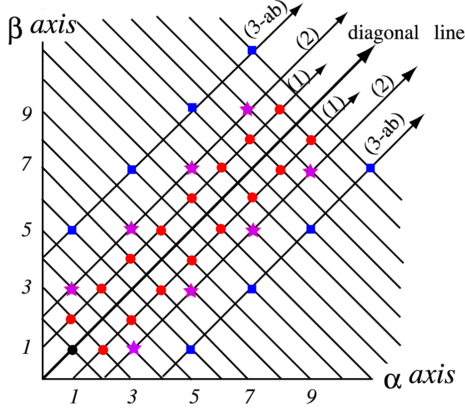
This implies that the minimal entropy among elements of Δm−1​(ℕ)\Delta_{m-1}(\mathbb{N}) is realized by (k−1)​α+k​β(k-1)\alpha+k\beta or k​α+(k−1)​βk\alpha+(k-1)\beta if m=2​km=2k. (See Figure 7.) The proof for other cases can be shown in a similar way. □\Box
Refer to caption
Figure 7: the first quadrant of α​β\alpha\beta plane. homology classes in (1) (resp. (2), (3a, 3b) of Prop. 3.29) lie on the lines →(1)\xrightarrow{\hskip 5.69054pt(1)} (resp. →(2)\xrightarrow{\hskip 5.69054pt(2)} and →(3−a​b)\xrightarrow{\hskip 5.69054pt(3-ab)}).
Lemma 3.17.

For k′>k>0k^{\prime}>k>0, we have the following.

(1)

ent¯​(k​α+(k+c)​β)>ent¯​(k′​α+(k′+c)​β)\overline{\mathrm{ent}}(k\alpha+(k+c)\beta)>\overline{\mathrm{ent}}(k^{\prime}\alpha+(k^{\prime}+c)\beta).

(2)

ent⁡(k​α+(k+c)​β)>ent⁡(k′​α+(k′+c)​β).\mathrm{ent}(k\alpha+(k+c)\beta)>\mathrm{ent}(k^{\prime}\alpha+(k^{\prime}+c)\beta).

Proof. For any k>0k>0, we have

ent¯​(k​α+(k+c)​β2​k+c)=ent⁡(k​α+(k+c)​β2​k+c)=(2​k+c)​ent​(k​α+(k+c)​β).\overline{\mathrm{ent}}(\tfrac{k\alpha+(k+c)\beta}{2k+c})=\mathrm{ent}(\tfrac{k\alpha+(k+c)\beta}{2k+c})=(2k+c)\mathrm{ent}(k\alpha+(k+c)\beta).

If 0<k<k′0<k<k^{\prime}, then c2​k+c>c2​k′+c\frac{c}{2k+c}>\frac{c}{2k^{\prime}+c}. By (3.7), we see that

ent⁡(k​α+(k+c)​β2​k+c)>ent⁡(k′​α+(k′+c)​β2​k′+c).\mathrm{ent}(\tfrac{k\alpha+(k+c)\beta}{2k+c})>\mathrm{ent}(\tfrac{k^{\prime}\alpha+(k^{\prime}+c)\beta}{2k^{\prime}+c}).

This implies (1). By (1),

ent⁡(k​α+(k+c)​β2​k+c)=(2​k+c)​ent​(k​α+(k+c)​β)\displaystyle\mathrm{ent}(\tfrac{k\alpha+(k+c)\beta}{2k+c})=(2k+c)\mathrm{ent}(k\alpha+(k+c)\beta)
>\displaystyle> ent⁡(k′​α+(k′+c)​β2​k′+c)=(2​k′+c)​ent​(k′​α+(k′+c)​β)\displaystyle\mathrm{ent}(\tfrac{k^{\prime}\alpha+(k^{\prime}+c)\beta}{2k^{\prime}+c})=(2k^{\prime}+c)\mathrm{ent}(k^{\prime}\alpha+(k^{\prime}+c)\beta)
>\displaystyle> (2​k+c)​ent​(k′​α+(k′+c)​β).\displaystyle(2k+c)\mathrm{ent}(k^{\prime}\alpha+(k^{\prime}+c)\beta).

Thus, ent⁡(k​α+(k+c)​β)>ent⁡(k′​α+(k′+c)​β)\mathrm{ent}(k\alpha+(k+c)\beta)>\mathrm{ent}(k^{\prime}\alpha+(k^{\prime}+c)\beta). This completes the proof of (2). □\Box

Proof of Proposition 3.12. (1) We consider the case n=2​k+1n=2k+1. For k=2k=2, we see that ℋ5={2​α+β}\mathcal{H}_{5}=\{2\alpha+\beta\}. If k≠2k\neq 2 and 2​k≡0(mod3)2k\equiv 0\pmod{3}, ℋ2​k+1\mathcal{H}_{2k+1} is the set of homology classes of type (1) of Corollary 3.10, that is

ℋ2​k+1={xα+yβ|xα+yβ∈Δ2​k−1(ℕ),x≥y}.\mathcal{H}_{2k+1}=\{x\alpha+y\beta\ |\ x\alpha+y\beta\in\Delta_{2k-1}(\mathbb{N}),\ x\geq y\}.

In this case, k​α+(k−1)​βk\alpha+(k-1)\beta reaches the minimal entropy among elements of ℋ2​k+1\mathcal{H}_{2k+1} by Lemma 3.16(1). Otherwise (i.e, 2​k≢0(mod3)2k\not\equiv 0\pmod{3}), ℋ2​k+1\mathcal{H}_{2k+1} is the union of homology classes of type (1) and (2) of Corollary 3.10:

{(2k−2)α+(2k−3)β+(2k−4)γ}∪{xα+yβ|xα+yβ∈Δ2​k−1(ℕ),x≥y}.\{(2k-2)\alpha+(2k-3)\beta+(2k-4)\gamma\}\cup\{x\alpha+y\beta\ |\ x\alpha+y\beta\in\Delta_{2k-1}(\mathbb{N}),\ x\geq y\}.

One needs to compare the entropy for (2​k−2)​α+(2​k−3)​β+(2​k−4)​γ(2k-2)\alpha+(2k-3)\beta+(2k-4)\gamma with the one for k​α+(k−1)​βk\alpha+(k-1)\beta. In case k=4k=4,

λ⁡(4​α+3​β)≈1.46557<λ⁡(6​α+5​β+4​γ)≈1.72208.\lambda(4\alpha+3\beta)\approx 1.46557<\lambda(6\alpha+5\beta+4\gamma)\approx 1.72208.

By Lemmas 3.17 and 3.13, for k>4k>4, we have

(2​k−1)​ent​(k​α+(k−1)​β)\displaystyle(2k-1)\mathrm{ent}(k\alpha+(k-1)\beta)
≤\displaystyle\leq 7​e​n​t​(4​α+3​β)\displaystyle 7\mathrm{ent}(4\alpha+3\beta)
<\displaystyle< 7​e​n​t​(6​α+5​β+4​γ)\displaystyle 7\mathrm{ent}(6\alpha+5\beta+4\gamma)
<\displaystyle< (2​k−1)​ent​((2​k−2)​α+(2​k−3)​β+(2​k−4)​γ).\displaystyle(2k-1)\mathrm{ent}((2k-2)\alpha+(2k-3)\beta+(2k-4)\gamma).

Thus, ent⁡(k​α+(k−1)​β)<ent⁡((2​k−2)​α+(2​k−3)​β+(2​k−4)​γ)\mathrm{ent}(k\alpha+(k-1)\beta)<\mathrm{ent}((2k-2)\alpha+(2k-3)\beta+(2k-4)\gamma). This completes the proof.

(2) Let us consider the case n=4​k+2n=4k+2. For k=1k=1, ℋ6={3​α+β,3​α+2​β+γ}\mathcal{H}_{6}=\{3\alpha+\beta,3\alpha+2\beta+\gamma\}. We have

λ⁡(3​α+2​β+γ)≈2.08102<λ⁡(3​α+β)≈2.29663.\lambda(3\alpha+2\beta+\gamma)\approx 2.08102<\lambda(3\alpha+\beta)\approx 2.29663.

For k=2k=2, ℋ10={7​α+4​β+3​γ,5​α+3​β,7​α+β}\mathcal{H}_{10}=\{7\alpha+4\beta+3\gamma,5\alpha+3\beta,7\alpha+\beta\}. We have inequalities

λ⁡(5​α+3​β)≈1.41345<λ⁡(7​α+4​β+3​γ)≈1.55603​and​λ​(5​α+3​β)<λ⁡(7​α+β).\lambda(5\alpha+3\beta)\approx 1.41345<\lambda(7\alpha+4\beta+3\gamma)\approx 1.55603\ \mbox{and}\ \lambda(5\alpha+3\beta)<\lambda(7\alpha+\beta).

For k=3k=3, ℋ14={11​α+6​β+5​γ,7​α+5​β,11​α+β,11​α+10​β+9​γ}\mathcal{H}_{14}=\{11\alpha+6\beta+5\gamma,7\alpha+5\beta,11\alpha+\beta,11\alpha+10\beta+9\gamma\}. We have λ⁡(7​α+5​β)<λ⁡(11​α+β)\lambda(7\alpha+5\beta)<\lambda(11\alpha+\beta) by Lemma 3.16(2) and

λ⁡(7​α+5​β)≈1.25141\displaystyle\lambda(7\alpha+5\beta)\approx 1.25141 <\displaystyle< λ⁡(11​α+6​β+5​γ)≈1.39241\displaystyle\lambda(11\alpha+6\beta+5\gamma)\approx 1.39241
<\displaystyle< λ⁡(11​α+10​β+9​γ)≈1.62913.\displaystyle\lambda(11\alpha+10\beta+9\gamma)\approx 1.62913.

By using the same arguments as in the case n=2​k+1n=2k+1, we have for all k>3k>3, (4​k)​ent​((2​k+1)​α+(2​k−1)​β)<12​ent​(7​α+5​β)(4k)\mathrm{ent}((2k+1)\alpha+(2k-1)\beta)<12\mathrm{ent}(7\alpha+5\beta) and

12​e​n​t​(11​α+6​β+5​γ)\displaystyle 12\mathrm{ent}(11\alpha+6\beta+5\gamma) <\displaystyle< (4​k)​ent​((4​k−1)​α+2​k​β+(2​k−1)​γ),\displaystyle(4k)\mathrm{ent}((4k-1)\alpha+2k\beta+(2k-1)\gamma),
12​e​n​t​(11​α+10​β+9​γ)\displaystyle 12\mathrm{ent}(11\alpha+10\beta+9\gamma) <\displaystyle< (4​k)​ent​((4​k−1)​α+(4​k−2)​β+(4​k−3)​γ).\displaystyle(4k)\mathrm{ent}((4k-1)\alpha+(4k-2)\beta+(4k-3)\gamma).

Thus, for all k≥2k\geq 2, (2​k+1)​α+(2​k−1)​β(2k+1)\alpha+(2k-1)\beta, which realizes the minimal entropy among elements of Δ4​k​(ℕ)\Delta_{4k}(\mathbb{N}), reaches the minimal entropy among elements of ℋ4​k+2\mathcal{H}_{4k+2}.

(3a) The proof for the case n=8​k+4n=8k+4 is shown in a similar way.

(3b) Let us consider the case n=8​(k+1)n=8(k+1). For k=0k=0, we see that ℋ8={5​α+3​β+2​γ,5​α+β,5​α+4​β+3​γ}\mathcal{H}_{8}=\{5\alpha+3\beta+2\gamma,5\alpha+\beta,5\alpha+4\beta+3\gamma\}, and

λ⁡(5​α+3​β+2​γ)≈1.72208<λ⁡(5​α+4​β+3​γ)≈1.78164<λ⁡(5​α+β)≈2.08102.\lambda(5\alpha+3\beta+2\gamma)\approx 1.72208<\lambda(5\alpha+4\beta+3\gamma)\approx 1.78164<\lambda(5\alpha+\beta)\approx 2.08102.

For k≥1k\geq 1, one can show that (4​k+5)​α+(4​k+1)​β(4k+5)\alpha+(4k+1)\beta reaches the minimal dilatation among elements of ℋ8​k+4\mathcal{H}_{8k+4}. □\Box

3.5 Monodromy

The braid Θ=Θm=(σ12σ2σ3⋯σm−1)m−1=(σ1σ2⋯σm−1)m∈Bm\Theta=\Theta_{m}=(\sigma_{1}^{2}\sigma_{2}\sigma_{3}\cdots\sigma_{m-1})^{m-1}=(\sigma_{1}\sigma_{2}\cdots\sigma_{m-1})^{m}\in B_{m} is the full twist. Hence we have:

Refer to caption
Figure 8: (left) braid T6,2T_{6,2}. (right) braid T5,2T_{5,2}.
Lemma 3.18.

If p≡p′(modm−1)p\equiv p^{\prime}\pmod{m-1}, then there exists an integer kk such that Tm,p=Tm,p′​ΘkT_{m,p}=T_{m,p^{\prime}}\Theta^{k} and Γ⁡(Tm,p)=Γ⁡(Tm,p′)∈ℳ⁡(Dm)\Gamma(T_{m,p})=\Gamma(T_{m,p^{\prime}})\in\mathcal{M}(D_{m}).

Let us consider the braid Tm,pT_{m,p} in case gcd⁡(m−1,p)≠1\gcd(m-1,p)\neq 1. For example, T5,2T_{5,2} is a reducible braid, since a disjoint union of two simple closed curves in D5D_{5} is invariant under Γ⁡(T5,2)\Gamma(T_{5,2}), see Figure 8(right). It is not hard to see the following.

Lemma 3.19.

If gcd⁡(m−1,p)≠1\gcd(m-1,p)\neq 1, then Tm,pT_{m,p} is a reducible braid.

Theorem 3.20.

Suppose that x​α+y​β∈Δm−1​(ℕ)x\alpha+y\beta\in\Delta_{m-1}({\mathbb{N}}) for m≥3m\geq 3. Then there exists p=p⁡(x,y)p=p(x,y) such that the braid Tm,pT_{m,p} is the monodromy on a fiber which is the minimal representative of x​α+y​βx\alpha+y\beta.

The rest of section is devoted to proving Theorem 3.20 and explaining how to compute p=p⁡(x,y)p=p(x,y).

3.5.1 Fiber surface

The aim of this section is to find fibers Fm⁡(q),p⁡(q)F_{m(q),p(q)} for the magic manifold associated to sequences of natural numbers qq whose homology class [Fm⁡(q),p⁡(q)][F_{m(q),p(q)}] is in CΔ1​(ℤ)C_{\Delta_{1}}({\mathbb{Z}}).

Let LL be a link in S3S^{3}. Let E1E_{1} be an oriented disk with punctures which is embedded in the exterior E⁡(L)=S3∖𝒩⁡(L)E(L)=S^{3}\setminus\mathcal{N}(L) of LL and let E2E_{2} be any embedded, oriented surface in E⁡(L)E(L) as in Figure 9(1). The oriented surface E1+E2E_{1}+E_{2}, which depends on the orientation of E1E_{1} and E2E_{2}, is either of type (3) or type (4) in Figure 9. The front (resp. back) of E1+E2E_{1}+E_{2} is dark-colored (resp. light-colored) in the figure.

Suppose that E1+E2E_{1}+E_{2} is of type (3) (resp. (4)). Now, open E⁡(L)E(L) along E1E_{1}, and let E′E^{\prime} and E′′E^{\prime\prime} be the resulting punctured disks obtained from E1E_{1}. Reglue E′E^{\prime} and E′′E^{\prime\prime} by twisting one of the disks by 360×N360\times N degrees in the clockwise (resp. counterclockwise) direction for some N∈ℕN\in{\mathbb{N}}. Then we obtain a new link, call it L′L^{\prime} such that E⁡(L′)≃E⁡(L)E(L^{\prime})\simeq E(L) (i.e, E⁡(L′)E(L^{\prime}) is homeomorphic to E⁡(L)E(L)). Let (E1′,E2′)(E_{1}^{\prime},E_{2}^{\prime}) be the ordered pair of the embedded, oriented surfaces in E⁡(L)E(L) which are obtained from the ordered pair (E1,E2)(E_{1},E_{2}) (see Figure 9(2)). The orientations of E1′E_{1}^{\prime} and E2′E_{2}^{\prime} are induced from E1E_{1} and E2E_{2} respectively.

Lemma 3.21.

Let L,L′L,L^{\prime} be the links, Ei,Ei′E_{i},E^{\prime}_{i} (i=1,2)(i=1,2) be the surfaces as above and let N∈𝐍N\in{\bf N} as above. There exists an orientation preserving homeomorphism f:E⁡(L)→E⁡(L′)f:E(L)\rightarrow E(L^{\prime}) such that

(1)

f⁡(y​E1+x​E2)=r​E1′+x​E2′f(yE_{1}+xE_{2})=rE_{1}^{\prime}+xE_{2}^{\prime} and

(2)

f⁡(E1)=E1′f(E_{1})=E_{1}^{\prime},

where y=x​N+ry=xN+r for x,y∈ℕx,y\in{\mathbb{N}} and 0≤r<x0\leq r<x. In particular,

(1’)

f⁡(N​E1+E2)=E2′f(NE_{1}+E_{2})=E_{2}^{\prime}.

Proof. The construction of L′L^{\prime} implies the existence of a homeomorphism f:E⁡(L)→E⁡(L′)f:E(L)\rightarrow E(L^{\prime}) with the properties (1) and (2). (By using Figure 9(3) and (4), one easily sees that f⁡(E1+E2)=E2′f(E_{1}+E_{2})=E_{2}^{\prime} and f⁡(E1)=E1′f(E_{1})=E_{1}^{\prime}. One can generalize the first equality to the claim (1).) □\Box

Note that by Lemma 3.21, ([E1′],[E2′])=([E1],[N​E1+E2])([E_{1}^{\prime}],[E_{2}^{\prime}])=([E_{1}],[NE_{1}+E_{2}]).

Refer to caption
Figure 9: (1) E1E_{1}, E2↪E⁡(L)E_{2}\hookrightarrow E(L). (2) E1′E_{1}^{\prime}, E2′↪E⁡(L′)E_{2}^{\prime}\hookrightarrow E(L^{\prime}) (in case N=2N=2 in Lemma 3.21). (3) and (4) E1+E2↪E⁡(L)E_{1}+E_{2}\hookrightarrow E(L).

Let us consider the exterior of the braided link E⁡(T¯m,p)E(\overline{T}_{m,p}). Now, we shall define two oriented surfaces F^m,p\widehat{F}_{m,p}, Fm,p↪E⁡(T¯m,p)F_{m,p}\hookrightarrow E(\overline{T}_{m,p}) whose orientations are induced by the oriented link T¯m,p\overline{T}_{m,p}. (Recall that the orientation of T¯m,p\overline{T}_{m,p} is given as in Figure 2(right).) The oriented surface Fm,pF_{m,p} is an mm-punctured disk which is bounded by the braid axis of Tm,pT_{m,p}, see Figure 10(left). Clearly, Fm,pF_{m,p} is a fiber for E⁡(T¯m,p)E(\overline{T}_{m,p}) with the monodromy Tm,pT_{m,p}. The oriented surface F^m,p\widehat{F}_{m,p} is a (p+1)(p+1)-punctured disk which is bounded by Km,pK_{m,p}, where Km,pK_{m,p} is the knot which is the closing the 11st strand of Tm,pT_{m,p}, see Figure 10(right).

Refer to caption
Figure 10: Fm,pF_{m,p}, F^m,p↪E⁡(T¯m,p)\widehat{F}_{m,p}\hookrightarrow E(\overline{T}_{m,p}) in case (m,p)=(5,1)(m,p)=(5,1). (one sees that F^5,1\widehat{F}_{5,1} is a twice-punctured disk.)

Given m,p∈ℕm,p\in{\mathbb{N}} and (k,ℓ)∈ℕ×ℕ(k,\ell)\in{\mathbb{N}}\times{\mathbb{N}}, the following construction enables us to see another fiber Fm′,p′↪E⁡(T¯m,p)F_{m^{\prime},p^{\prime}}\hookrightarrow E(\overline{T}_{m,p}) with the monodromy Tm′,p′T_{m^{\prime},p^{\prime}}.

(Construction of fibers.)

Step 1. Apply Lemma 3.21 for the link T¯m,p\overline{T}_{m,p}, the ordered pair (E1,E2)=(Fm,p,F^m,p)(E_{1},E_{2})=(F_{m,p},\widehat{F}_{m,p}) and N=kN=k. (Note that Fm,pF_{m,p} is a disk with punctures and hence one can apply Lemma 3.21.) Then we obtain the ordered pair of embedded surfaces in E⁡(T¯m,p)E(\overline{T}_{m,p});

(Fm,k⁡(m−1)+p,F^m,k⁡(m−1)+p)=(Fm,p,k​Fm,p+F^m,p).(F_{m,k(m-1)+p},\widehat{F}_{m,k(m-1)+p})=(F_{m,p},kF_{m,p}+\widehat{F}_{m,p}).

(Notice that Θk=(σ12σ2σ3⋯σm−1)k⁡(m−1)\Theta^{k}=(\sigma_{1}^{2}\sigma_{2}\sigma_{3}\cdots\sigma_{m-1})^{k(m-1)}.)

Step 2. Apply Lemma 3.21 for the link T¯m,k⁡(m−1)+p\overline{T}_{m,k(m-1)+p}, the ordered pair (E1,E2)=(F^m,k⁡(m−1)+p,Fm,k⁡(m−1)+p)(E_{1},E_{2})=(\widehat{F}_{m,k(m-1)+p},F_{m,k(m-1)+p}) and N=ℓN=\ell. (Note that F^m,k⁡(m−1)+p\widehat{F}_{m,k(m-1)+p} is a disk with punctures and hence one can apply the lemma.) Then it turns out that the new link L′=L′​(T¯m,k⁡(m−1)+p)L^{\prime}=L^{\prime}(\overline{T}_{m,k(m-1)+p}) is isotopic to T¯m′,p′\overline{T}_{m^{\prime},p^{\prime}}, and we obtain the ordered pair of embedded surfaces in E⁡(T¯m,p)E(\overline{T}_{m,p});

(F^m′,p′,Fm′,p′)=(F^m,k⁡(m−1)+p,ℓ​F^m,k⁡(m−1)+p+Fm,k⁡(m−1)+p),(\widehat{F}_{m^{\prime},p^{\prime}},F_{m^{\prime},p^{\prime}})=(\widehat{F}_{m,k(m-1)+p},\ell\widehat{F}_{m,k(m-1)+p}+F_{m,k(m-1)+p}), (3.8)

where

m′\displaystyle m^{\prime} =\displaystyle= ℓ⁡(k⁡(m−1)+p)+m,\displaystyle\ell(k(m-1)+p)+m,
p′\displaystyle p^{\prime} =\displaystyle= k⁡(m−1)+p.\displaystyle k(m-1)+p.

Thus we have another fiber Fm′,p′F_{m^{\prime},p^{\prime}} for E⁡(T¯m,p)E(\overline{T}_{m,p}) with the monodromy Tm′​p′T_{m^{\prime}p^{\prime}}. (End of the construction.)

We sometimes denote m′m^{\prime} and p′p^{\prime} by m′​(m,p,k,ℓ)m^{\prime}(m,p,k,\ell) and p′​(m,p,k,ℓ)p^{\prime}(m,p,k,\ell).

For example, in case Tm,p=T5,1T_{m,p}=T_{5,1} and (k,ℓ)=(1,2)(k,\ell)=(1,2), we have Tm′,p′=T15,5T_{m^{\prime},p^{\prime}}=T_{15,5}, see Figure 13(2),(3),(4). ((3) explains Step 1 and (4) explains Step 2.)

By using Lemma 3.21, it is easy to see the following.

Proposition 3.22.

Let x,y∈ℕx,y\in{\mathbb{N}}. Suppose that 0<x<y0<x<y and y≢0(modx)y\not\equiv 0\pmod{x}. Take k,ℓ,r1,r2k,\ell,r_{1},r_{2} such that

y\displaystyle y =\displaystyle= xk+r1(0<r1<x,k∈ℕ),\displaystyle xk+r_{1}\ (0<r_{1}<x,\ k\in{\mathbb{N}}),
x\displaystyle x =\displaystyle= r1ℓ+r2(0≤r2<r1,ℓ∈ℕ).\displaystyle r_{1}\ell+r_{2}\ (0\leq r_{2}<r_{1},\ \ell\in{\mathbb{N}}).

We apply the construction of a fiber for a given m,p∈ℕm,p\in{\mathbb{N}} and such a pair (k,ℓ)(k,\ell). Then there exists an orientation preserving homeomorphism f:E⁡(T¯m,p)→E⁡(T¯m′,p′)f:E(\overline{T}_{m,p})\rightarrow E(\overline{T}_{m^{\prime},p^{\prime}}) such that

f⁡(x​F^m,p+y​Fm,p)=r2​F^m′,p′+r1​Fm′,p′.f(x\widehat{F}_{m,p}+yF_{m,p})=r_{2}\widehat{F}_{m^{\prime},p^{\prime}}+r_{1}F_{m^{\prime},p^{\prime}}.

Let q=(q1,q2,⋯,qt)q=(q_{1},q_{2},\cdots,q_{t}) be a sequence of natural numbers. The number tt in the sequence, denoted by |q||q|, is called the length of qq. For q=(k1,ℓ1,⋯,kj,ℓj)q=(k_{1},\ell_{1},\cdots,k_{j},\ell_{j}) with even length, let q|i=(k1,ℓ1,⋯,ki,ℓi)q|_{i}=(k_{1},\ell_{1},\cdots,k_{i},\ell_{i}) for i≤ji\leq j. For q=(ℓ0,k1,ℓ1,⋯,kj,ℓj)q=(\ell_{0},k_{1},\ell_{1},\cdots,k_{j},\ell_{j}) with odd length, let q|i=(ℓ0,k1,ℓ1,⋯,ki,ℓi)q|_{i}=(\ell_{0},k_{1},\ell_{1},\cdots,k_{i},\ell_{i}) for i≤ji\leq j. Note that q=q|jq=q|_{j}.

We will define a fiber Fm⁡(q),p⁡(q)F_{m(q),p(q)} for E⁡(𝒞3)E({\mathcal{C}}_{3}) with the monodromy Tm⁡(q),p⁡(q)T_{m(q),p(q)} associated to qq such that its homology class [Fm⁡(q),p⁡(q)][F_{m(q),p(q)}] is in CΔ1​(ℤ)C_{\Delta_{1}}({\mathbb{Z}}). To do so, we define a fiber Fm⁡(q|i),p⁡(q|i)F_{m(q|_{i}),p(q|_{i})} for E⁡(𝒞3)E({\mathcal{C}}_{3}) with the monodromy Tm⁡(q|i),p⁡(q|i)T_{m(q|_{i}),p(q|_{i})} inductively as follows. Another oriented diagram of 𝒞3{\mathcal{C}}_{3} is given in Figure 11(left). The oriented twice-punctured disk EαE_{\alpha} (resp. EβE_{\beta}) bounded by KαK_{\alpha} (KβK_{\beta}), whose orientation is induced by 𝒞3\mathcal{C}_{3} is a representative of α\alpha (resp. β\beta), see Figure 11(center, right). We first consider a sequence qq with even length.

Case 1 (even). Suppose that q=(k1,ℓ1)q=(k_{1},\ell_{1}). First, apply Lemma 3.21 for L=𝒞3L={\mathcal{C}}_{3}, the ordered pair (E1,E2)=(Eβ,Eα)(E_{1},E_{2})=(E_{\beta},E_{\alpha}) and N=k1N=k_{1}. Let (Eβ,k1​Eβ+Eα)(E_{\beta},k_{1}E_{\beta}+E_{\alpha}) be the ordered pair of embedded surface in E⁡(𝒞3)≃E⁡(L′)E(\mathcal{C}_{3})\simeq E(L^{\prime}) induced from (Eβ,Eα)(E_{\beta},E_{\alpha}). Second, apply Lemma 3.21 for L′L^{\prime}, the ordered pair (k1​Eβ+Eα,Eβ)(k_{1}E_{\beta}+E_{\alpha},E_{\beta}) and N=ℓ1N=\ell_{1}. Then we have the ordered pair of embedded surfaces

(k1​Eβ+Eα,ℓ1​(k1​Eβ+Eα)+Eβ)(k_{1}E_{\beta}+E_{\alpha},\ell_{1}(k_{1}E_{\beta}+E_{\alpha})+E_{\beta}) (3.9)

in E⁡(𝒞3)≃E⁡(L′′)E(\mathcal{C}_{3})\simeq E(L^{\prime\prime}), where L′′=(L′)′L^{\prime\prime}=(L^{\prime})^{\prime}. We see that L′′L^{\prime\prime} is a braided link of Tm⁡(q),p⁡(q)=T(k1+1)​ℓ1+2,k1+1T_{m(q),p(q)}=T_{(k_{1}+1)\ell_{1}+2,k_{1}+1}, and

(F^m⁡(q),p⁡(q),Fm⁡(q),p⁡(q))=(k1​Eβ+Eα,ℓ1​(k1​Eβ+Eα)+Eβ)(\widehat{F}_{m(q),p(q)},F_{m(q),p(q)})=(k_{1}E_{\beta}+E_{\alpha},\ell_{1}(k_{1}E_{\beta}+E_{\alpha})+E_{\beta}) (3.10)

by (3.9). Therefore Fm⁡(q),p⁡(q)F_{m(q),p(q)} is a fiber for E⁡(𝒞3)E({\mathcal{C}}_{3}) with the monodromy Tm⁡(q),p⁡(q)T_{m(q),p(q)}, and by (3.10),

[Fm⁡(q),p⁡(q)]=ℓ1​α+(ℓ1​k1+1)​β∈CΔ1​(ℤ)\left[F_{m(q),p(q)}\right]=\ell_{1}\alpha+(\ell_{1}k_{1}+1)\beta\in C_{\Delta_{1}}(\mathbb{Z})

since α=[Eα]\alpha=[E_{\alpha}] and β=[Eβ]\beta=[E_{\beta}]. For example in case q=(1,1)q=(1,1), we have Tm⁡(q),p⁡(q)=T4,2T_{m(q),p(q)}=T_{4,2}, see Figure 12.

Suppose that q=(k1,ℓ1,⋯,kj,ℓj)q=(k_{1},\ell_{1},\cdots,k_{j},\ell_{j}), j>1j>1. For i=1i=1, we have defined a fiber Fm⁡(q|1),p⁡(q|1)F_{m(q|_{1}),p(q|_{1})} for E⁡(𝒞3)E({\mathcal{C}}_{3}) with the monodromy Tm⁡(q|1),p⁡(q|1)T_{m(q|_{1}),p(q|_{1})} as above. Suppose that we have a fiber Fm⁡(q|i),p⁡(q|i)F_{m(q|_{i}),p(q|_{i})} for E⁡(𝒞3)≃E⁡(T¯m⁡(q|i),p⁡(q|i))E({\mathcal{C}}_{3})\simeq E(\overline{T}_{m(q|_{i}),p(q|_{i})}) with the monodromy Tm⁡(q|i),p⁡(q|i)T_{m(q|_{i}),p(q|_{i})}. Apply the construction of a fiber for T¯m⁡(q|i),p⁡(q|i)\overline{T}_{m(q|_{i}),p(q|_{i})} and the pair (ki+1,ℓi+1)(k_{i+1},\ell_{i+1}). Then we have the ordered pair of embedded surfaces (F^m⁡(q|i+1),p⁡(q|i+1),Fm⁡(q|i+1),p⁡(q|i+1))(\widehat{F}_{m(q|_{i+1}),p(q|_{i+1})},\ F_{m(q|_{i+1}),p(q|_{i+1})}) in E⁡(𝒞3)E({\mathcal{C}}_{3}) (given in Step 2 in the construction) which is defined by

(F^m⁡(q|i+1),p⁡(q|i+1),Fm⁡(q|i+1),p⁡(q|i+1))=(F^m′,p′,Fm′,p′),\displaystyle(\widehat{F}_{m(q|_{i+1}),p(q|_{i+1})},F_{m(q|_{i+1}),p(q|_{i+1})})=(\widehat{F}_{m^{\prime},p^{\prime}},F_{m^{\prime},p^{\prime}}),

where m′=m′​(m⁡(q|i),p⁡(q|i),ki+1,ℓi+1)m^{\prime}=m^{\prime}(m(q|_{i}),p(q|_{i}),k_{i+1},\ell_{i+1}), p′=p′​(m⁡(q|i),p⁡(q|i),ki+1,ℓi+1)p^{\prime}=p^{\prime}(m(q|_{i}),p(q|_{i}),k_{i+1},\ell_{i+1}), see (3.8). The surface Fm⁡(q|i+1),p⁡(q|i+1)F_{m(q|_{i+1}),p(q|_{i+1})} is a fiber for E⁡(𝒞3)E({\mathcal{C}}_{3}) with the monodromy Tm⁡(q|i+1),p⁡(q|i+1)T_{m(q|_{i+1}),p(q|_{i+1})}. By induction, it is shown that [Fm⁡(q|i+1),p⁡(q|i+1)]∈CΔ1​(ℤ)\left[F_{m(q|_{i+1}),p(q|_{i+1})}\right]\in C_{\Delta_{1}}(\mathbb{Z}).

Next, let us consider a sequence qq with odd length.

Case 2 (odd). Suppose that q=(ℓ0)q=(\ell_{0}). Applying Lemma 3.21 for L=𝒞3L={\mathcal{C}}_{3}, the ordered pair (E1,E2)=(Eα,Eβ)(E_{1},E_{2})=(E_{\alpha},E_{\beta}) (not (E1,E2)=(Eβ,Eα)(E_{1},E_{2})=(E_{\beta},E_{\alpha}) as in Case 1 (even)) and N=ℓ0N=\ell_{0}, we obtain the ordered pair of embedded surfaces (Eα,ℓ0​Eα+Eβ)(E_{\alpha},\ell_{0}E_{\alpha}+E_{\beta}) in E⁡(𝒞3)≃E⁡(L′)E(\mathcal{C}_{3})\simeq E(L^{\prime}). We see that L′L^{\prime} is a braided link of Tm⁡(q),p⁡(q)=Tℓ0+2,1T_{m(q),p(q)}=T_{\ell_{0}+2,1}. We have

(F^m⁡(q),p⁡(q),Fm⁡(q),p⁡(q))=(Eα,ℓ0​Eα+Eβ).(\widehat{F}_{m(q),p(q)},F_{m(q),p(q)})=(E_{\alpha},\ell_{0}E_{\alpha}+E_{\beta}).

Therefore Fm⁡(q),p⁡(q)F_{m(q),p(q)} is a fiber for E⁡(𝒞3)E({\mathcal{C}}_{3}) with the monodromy Tm⁡(q),p⁡(q)T_{m(q),p(q)}, and

[Fm⁡(q),p⁡(q)]=ℓ0​α+β∈CΔ1​(ℤ).\left[F_{m(q),p(q)}\right]=\ell_{0}\alpha+\beta\in C_{\Delta_{1}}(\mathbb{Z}).

In case ℓ0=3\ell_{0}=3, see Figure 13(2).

Suppose that q=(ℓ0,k1,ℓ1,⋯,kj,ℓj)q=(\ell_{0},k_{1},\ell_{1},\cdots,k_{j},\ell_{j}), 2​j+1>12j+1>1. For i=0i=0, we have defined a fiber Fm⁡(q|0),p⁡(q|0)F_{m(q|_{0}),p(q|_{0})} for E⁡(𝒞3)≃E⁡(T¯m⁡(0),p⁡(0))E({\mathcal{C}}_{3})\simeq E(\overline{T}_{m(0),p(0)}) with the monodromy Tm⁡(q|0),p⁡(q|0)T_{m(q|_{0}),p(q|_{0})} as above. For i≥1i\geq 1, in the same manner as Case 1 (even), a fiber Fm⁡(q|i),p⁡(q|i)F_{m(q|_{i}),p(q|_{i})} for E⁡(𝒞3)E({\mathcal{C}}_{3}) with the monodromy Tm⁡(q|i),p⁡(q|i)T_{m(q|_{i}),p(q|_{i})} is given inductively, and we see that [Fm⁡(q),p⁡(q)]∈CΔ1​(ℤ)\left[F_{m(q),p(q)}\right]\in C_{\Delta_{1}}(\mathbb{Z}). In case q=(3,1,2)q=(3,1,2), see Figure 13.

Refer to caption
Figure 11: (left) 𝒞3\mathcal{C}_{3}. (center), (right) EαE_{\alpha}, Eβ↪E⁡(𝒞3)E_{\beta}\hookrightarrow E(\mathcal{C}_{3}).
Refer to caption
Figure 12: fiber F4,2F_{4,2} with monodromy T4,2T_{4,2} associated to (1,1)(1,1). (2) and (3) describe the first and second part of Case 1 (even) respectively.
Refer to caption
Figure 13: construction of fiber F15,5F_{15,5} associated to (3,1,2)(3,1,2). (1) 𝒞3\mathcal{C}_{3}. (2) T¯5,1\overline{T}_{5,1}. (fiber F5,1F_{5,1} associated to q=(3)q=(3).) (3) T¯5,5\overline{T}_{5,5}. (4) T¯15,5\overline{T}_{15,5}.

3.5.2 Continued fraction

Let us consider a continued fraction with length jj

w1+1w2​+​1w3​+⋯+​1wj−1​+​1wj​:=w1+1w2+1w3+⋯1wj−1+1wjw_{1}+\frac{1}{w_{2}}{\genfrac{}{}{0.0pt}{}{}{+}}\frac{1}{w_{3}}{\genfrac{}{}{0.0pt}{}{}{+ \cdots+}}\frac{1}{w_{j-1}}{\genfrac{}{}{0.0pt}{}{}{+}}\frac{1}{w_{j}}{\genfrac{}{}{0.0pt}{}{}{}}:=w_{1}+\cfrac{1}{w_{2}+\cfrac{1}{w_{3}+\cdots\cfrac{1}{w_{j-1}+\cfrac{1}{w_{j}}}}}

for wi∈ℕw_{i}\in{\mathbb{N}}. We define [w1,w2,⋯,wj]∈ℕ\left[w_{1},w_{2},\cdots,w_{j}\right]\in{\mathbb{N}} inductively as follows.

[w1]\displaystyle\left[w_{1}\right] =\displaystyle= w1,\displaystyle w_{1},
[w1,w2]\displaystyle\left[w_{1},w_{2}\right] =\displaystyle= w1​w2+1,\displaystyle w_{1}w_{2}+1,
[w1,w2,⋯,wi]\displaystyle\left[w_{1},w_{2},\cdots,w_{i}\right] =\displaystyle= [w1,w2,⋯,wi−1]​wi+[w1,w2,⋯,wi−2].\displaystyle\left[w_{1},w_{2},\cdots,w_{i-1}\right]w_{i}+\left[w_{1},w_{2},\cdots,w_{i-2}\right].

The following is elementary and well-known.

Lemma 3.23.
(1)

w1+1w2​+​1w3​+⋯+​1wj−1​+​1wj​=[w1,w2,⋯,wj][w2,w3,⋯,wj]w_{1}+\frac{1}{w_{2}}{\genfrac{}{}{0.0pt}{}{}{+}}\frac{1}{w_{3}}{\genfrac{}{}{0.0pt}{}{}{+ \cdots+}}\frac{1}{w_{j-1}}{\genfrac{}{}{0.0pt}{}{}{+}}\frac{1}{w_{j}}{\genfrac{}{}{0.0pt}{}{}{}}=\frac{\left[w_{1},w_{2},\cdots,w_{j}\right]}{\left[w_{2},w_{3},\cdots,w_{j}\right]}.

(2)

[w1,w2,⋯,wj]=[wj,wj−1,⋯,w1]\left[w_{1},w_{2},\cdots,w_{j}\right]=\left[w_{j},w_{j-1},\cdots,w_{1}\right].

Definition 3.24.

Suppose that gcd⁡(u,v)=1\gcd(u,v)=1 for u,v∈ℕu,v\in{\mathbb{N}}. We define two sequences of non-negative integers r=(r0,r1,⋯,rj+1)r=(r_{0},r_{1},\cdots,r_{j+1}) and q=(q1,q2,⋯,qj)q=(q_{1},q_{2},\cdots,q_{j}) associated to {u,v}\{u,v\} (according to the Euclidean algorithm). We set r0=max⁡{u,v}r_{0}=\max\{u,v\} and r1=min⁡{u,v}r_{1}=\min\{u,v\}. Write r0=r1​q1+r2r_{0}=r_{1}q_{1}+r_{2} (0≤r2<r10\leq r_{2}<r_{1}).

  • •

    If r2=0r_{2}=0, then r1r_{1} must be 11 since gcd⁡(u,v)=1\gcd(u,v)=1. We set

    r=(r0,r1=1,r2=0)​and​q=(q1).r=(r_{0},r_{1}=1,r_{2}=0)\ \mbox{and}\ q=(q_{1}).
  • •

    Suppose that r2≠0r_{2}\neq 0. We define q2,q3,⋯q_{2},q_{3},\cdots and r3,r4,⋯r_{3},r_{4},\cdots inductively as follows. Let qi>0q_{i}>0 and ri+1≥0r_{i+1}\geq 0 such that ri−1=ri​qi+ri+1r_{i-1}=r_{i}q_{i}+r_{i+1} (0≤ri+1<ri0\leq r_{i+1}<r_{i}). Since r0>⋯>ri>ri+1≥0r_{0}>\cdots>r_{i}>r_{i+1}\geq 0, there exists jj such that rj+1=0r_{j+1}=0. (Then rjr_{j} must be 11 since gcd⁡(u,v)=1\gcd(u,v)=1.) We set

    r=(r0,r1,⋯,rj=1,rj+1=0)​and​q=(q0,⋯,qj).r=(r_{0},r_{1},\cdots,r_{j}=1,r_{j+1}=0)\ \mbox{and}\ q=(q_{0},\cdots,q_{j}).

By using the sequence qq, the fraction max⁡{u,v}min⁡{u,v}\frac{\max\{u,v\}}{\min\{u,v\}} can be expressed by the following two kinds of continued fractions.

max⁡{u,v}min⁡{u,v}\displaystyle\frac{\max\{u,v\}}{\min\{u,v\}} =\displaystyle= q1+1q2​+​1q3​+⋯+​1qj−1​+​1qj​,\displaystyle q_{1}+\frac{1}{q_{2}}{\genfrac{}{}{0.0pt}{}{}{+}}\frac{1}{q_{3}}{\genfrac{}{}{0.0pt}{}{}{+ \cdots+}}\frac{1}{q_{j-1}}{\genfrac{}{}{0.0pt}{}{}{+}}\frac{1}{q_{j}}{\genfrac{}{}{0.0pt}{}{}{}}, (3.11)
max⁡{u,v}min⁡{u,v}\displaystyle\frac{\max\{u,v\}}{\min\{u,v\}} =\displaystyle= q1+1q2​+​1q3​+⋯+​1qj−1​+​1(qj−1)​+​11​\displaystyle q_{1}+\frac{1}{q_{2}}{\genfrac{}{}{0.0pt}{}{}{+}}\frac{1}{q_{3}}{\genfrac{}{}{0.0pt}{}{}{+ \cdots+}}\frac{1}{q_{j-1}}{\genfrac{}{}{0.0pt}{}{}{+}}\frac{1}{(q_{j}-1)}{\genfrac{}{}{0.0pt}{}{}{+}}\frac{1}{1}{\genfrac{}{}{0.0pt}{}{}{}} (3.12)

with length jj and j+1j+1 respectively. We can choose the one with odd/even length among those continued fractions.

Proof of Theorem 3.20. Let x​α+y​β∈Δm−1​(ℕ)x\alpha+y\beta\in\Delta_{m-1}({\mathbb{N}}). (By the definition of Δm−1​(ℕ)\Delta_{m-1}({\mathbb{N}}), xx and yy are relatively prime.) From the continued fractions of max⁡{x,y}min⁡{x,y}\frac{\max\{x,y\}}{\min\{x,y\}} of the forms in (3.11) and (3.12) (constructed by one of the sequence (q1,q2,⋯)=(w1,w2,⋯)(q_{1},q_{2},\cdots)=(w_{1},w_{2},\cdots) in Definition 3.24 associated to {x,y}\{x,y\}), we choose the one with odd length if x>yx>y (resp. even length if x<yx<y):

max⁡{x,y}min⁡{x,y}=w1+1w2​+​1w3​+⋯+​1wj−1​+​1wj​.\frac{\max\{x,y\}}{\min\{x,y\}}=w_{1}+\frac{1}{w_{2}}{\genfrac{}{}{0.0pt}{}{}{+}}\frac{1}{w_{3}}{\genfrac{}{}{0.0pt}{}{}{+ \cdots+}}\frac{1}{w_{j-1}}{\genfrac{}{}{0.0pt}{}{}{+}}\frac{1}{w_{j}}{\genfrac{}{}{0.0pt}{}{}{}}. (3.13)

Now, we take s=(s0,s1,⋯,sj+1)s=(s_{0},s_{1},\cdots,s_{j+1}) which is defined by

s0\displaystyle s_{0} =\displaystyle= max⁡{x,y},\displaystyle\max\{x,y\},
s1\displaystyle s_{1} =\displaystyle= min⁡{x,y},\displaystyle\min\{x,y\},
si+1\displaystyle s_{i+1} =\displaystyle= si−1−si​wi​for ​i≥1.\displaystyle s_{i-1}-s_{i}w_{i}\ \mbox{for\ }i\geq 1.

Notice that sj=1s_{j}=1 and sj+1=0s_{j+1}=0. (If the continued fraction in (3.13) is of type (3.11), then ss equals rr in Definition 3.24.)

Suppose that x<yx<y. (In this case, the continued fraction of (3.13) has even length.) Let us write q=(w1,w2,⋯,wj)=(k1,ℓ1,⋯,kj/2,ℓj/2)q=(w_{1},w_{2},\cdots,w_{j})=(k_{1},\ell_{1},\cdots,k_{j/2},\ell_{j/2}). It is enough to show that a fiber Fm⁡(q),p⁡(q)F_{m(q),p(q)} for E⁡(𝒞3)E(\mathcal{C}_{3}) associated to qq is a representative of x​α+y​βx\alpha+y\beta. (If this is the case, Fm⁡(q),p⁡(q)F_{m(q),p(q)} is the minimal representative of x​α+y​βx\alpha+y\beta since Fm⁡(q),p⁡(q)F_{m(q),p(q)} is a fiber.) By using Proposition 3.22 repeatedly, we have

x​α+y​β\displaystyle x\alpha+y\beta =\displaystyle= [x​Eα+y​Eβ](=[s1​Eα+s0​Eβ])\displaystyle\left[xE_{\alpha}+yE_{\beta}\right](=\left[s_{1}E_{\alpha}+s_{0}E_{\beta}\right])
=\displaystyle= [s3​F^m⁡(q|1),p⁡(q|1)+s2​Fm⁡(q|1),p⁡(q|1)]\displaystyle\left[s_{3}\widehat{F}_{m(q|_{1}),p(q|_{1})}+s_{2}F_{m(q|_{1}),p(q|_{1})}\right]
=\displaystyle= [sj+1​F^m⁡(q|j/2),p⁡(q|j/2)+sj​Fm⁡(q|j/2),p⁡(q|j/2)]\displaystyle\left[s_{j+1}\widehat{F}_{m(q|_{j/2}),p(q|_{j/2})}+s_{j}F_{m(q|_{j/2}),p(q|_{j/2})}\right]
=\displaystyle= [0​F^m⁡(q|j/2),p⁡(q|j/2)+1​Fm⁡(q|j/2),p⁡(q|j/2)]\displaystyle\left[0\widehat{F}_{m(q|_{j/2}),p(q|_{j/2})}+1F_{m(q|_{j/2}),p(q|_{j/2})}\right]
=\displaystyle= [Fm⁡(q),p⁡(q)].\displaystyle\left[F_{m(q),p(q)}\right].

Since the minimal representative of x​α+y​βx\alpha+y\beta is an (x+y+2)(x+y+2)-punctured sphere, m⁡(q)m(q) equals x+y+1(=m)x+y+1(=m).

The proof for the case x>yx>y is similar. □\Box

3.5.3 Computation of p=p⁡(x,y)p=p(x,y) in Theorem 3.20

In this section we give a recipe to compute pp in Theorem 3.20. In Example 3.25, we explain how the number pp is related to the pair (x,y)(x,y).

Recall that Km,pK_{m,p} is the knot obtained by the closing the 11st strand of Tm,pT_{m,p}. Let Km,p♢K_{m,p}^{\diamondsuit} be the knot obtained by the closing the rest of strands, i.e, Km,p♢K_{m,p}^{\diamondsuit} equals the closed braid of Tm,pT_{m,p} with Km,pK_{m,p} removed. For the braided link T¯m,p\overline{T}_{m,p}, we have a pair of natural numbers

(i⁡(F^m,p,Km,p♢),i⁡(Fm,p,Km,p♢))=(p,m−1),(i(\widehat{F}_{m,p},K_{m,p}^{\diamondsuit}),i(F_{m,p},K_{m,p}^{\diamondsuit}))=(p,m-1),

where i⁡(S,K)i(S,K) is the intersection number between the surface SS and the knot KK. For 𝒞3\mathcal{C}_{3}, we have

(i⁡(Eα,Kγ),i⁡(Eβ,Kγ))=(1,1),(i(E_{\alpha},K_{\gamma}),i(E_{\beta},K_{\gamma}))=(1,1),

see Figure 11.

Example 3.25.

By the proof of Theorem 3.20 (see also the argument in Case 2 (odd) in Section 3.5.1 and Figure 13), T15,5T_{15,5} is the monodromy on a fiber which is the minimal representative for 11​α+3​β11\alpha+3\beta. We explain why p=5p=5 is derived from q=(q1,q2,q3)=(3,1,2)q=(q_{1},q_{2},q_{3})=(3,1,2) and r=(r0,r1,r2,r3,r4)=(11,3,2,1,0)r=(r_{0},r_{1},r_{2},r_{3},r_{4})=(11,3,2,1,0) of Definition 3.24 associated to {3,11}\{3,11\}. We have

[11​Eα+3​Eβ]=[2​F^5,1+3​F5,1]=[2​F^5,5+1​F5,5]=[0​F^15,5+1​F15,5].\left[11E_{\alpha}+3E_{\beta}\right]=\left[2\widehat{F}_{5,1}+3F_{5,1}\right]=\left[2\widehat{F}_{5,5}+1F_{5,5}\right]=\left[0\widehat{F}_{15,5}+1F_{15,5}\right].

The following is a simple description of these equalities.

(r0,r1)(r2,r1)(r2,r3)(r4,r3)∥∥∥∥(11,3)→q1=3(2,3)→q2=1(2,1)→q3=2(0,1)\left.\begin{array}[]{ccccccc}(r_{0},r_{1})&&(r_{2},r_{1})&&(r_{2},r_{3})&&(r_{4},r_{3})\\ \parallel&&\parallel&&\parallel&&\parallel\\ (11,3)&\xrightarrow[\ q_{1}=3\ ]{}&(2,3)&\xrightarrow[\ q_{2}=1\ ]{}&(2,1)&\xrightarrow[\ q_{3}=2\ ]{}&(0,1)\end{array}\right. (3.14)

In the process to find the fiber associated to q=(3,1,2)q=(3,1,2), we can find a sequence of pairs of intersection numbers (1,1)(1,1), (1,4)(1,4), (5,4)(5,4), (5,14)(5,14) obtained from 𝒞3\mathcal{C}_{3}, T¯5,1\overline{T}_{5,1}, T¯5,5\overline{T}_{5,5}, T¯15,5\overline{T}_{15,5} respectively which is described from left to right as follows.

(1,1)←q1=3(1,4)←q2=1(5,4)←q3=2(5,14)\left.\begin{array}[]{ccccccc}(1,1)&\xleftarrow[\ q_{1}=3\ ]{}&(1,4)&\xleftarrow[\ q_{2}=1\ ]{}&(5,4)&\xleftarrow[\ q_{3}=2\ ]{}&(5,14)\end{array}\right. (3.15)

Hence we can compute the number p=5p=5 from the sequence q=(3,1,2)q=(3,1,2). To describe the number pp explicitly, we extend the sequence of (3.14) to the left according to the Euclidean algorithm:

(r0,r0+r1)(r0,r1)(r2,r1)(r2,r3)(r4,r3)∥∥∥∥∥(11,14)→q0=1(11,3)→q1=3(2,3)→q2=1(2,1)→q3=2(0,1)\displaystyle\begin{array}[]{ccccccccc}(r_{0},r_{0}+r_{1})&&(r_{0},r_{1})&&(r_{2},r_{1})&&(r_{2},r_{3})&&(r_{4},r_{3})\\ \parallel&&\parallel&&\parallel&&\parallel&&\parallel\\ (11,14)&\xrightarrow[q_{0}=1]{}&(11,3)&\xrightarrow[q_{1}=3]{}&(2,3)&\xrightarrow[q_{2}=1]{}&(2,1)&\xrightarrow[q_{3}=2]{}&(0,1)\end{array}

In the same way, we extend the sequence of (3.15) to the left:

(0,1)←q0=1(1,1)←q1=3(1,4)←q2=1(5,4)←q3=2(5,14)\displaystyle\left.\begin{array}[]{ccccccccc}(0,1)&\xleftarrow[\ q_{0}=1\ ]{}&(1,1)&\xleftarrow[\ q_{1}=3\ ]{}&(1,4)&\xleftarrow[\ q_{2}=1\ ]{}&(5,4)&\xleftarrow[\ q_{3}=2\ ]{}&(5,14)\end{array}\right.

These show that

1411\displaystyle\frac{14}{11} =\displaystyle= 1+13​+​11​+​12​=[1,3,1,2][3,1,2]=[q0,q1,q2,q3][q1,q2,q3],\displaystyle 1+\frac{1}{3}{\genfrac{}{}{0.0pt}{}{}{+}}\frac{1}{1}{\genfrac{}{}{0.0pt}{}{}{+}}\frac{1}{2}{\genfrac{}{}{0.0pt}{}{}{}}=\frac{\left[1,3,1,2\right]}{\left[3,1,2\right]}=\frac{\left[q_{0},q_{1},q_{2},q_{3}\right]}{\left[q_{1},q_{2},q_{3}\right]},
145\displaystyle\frac{14}{5} =\displaystyle= 2+11​+​13​+​11​=[2,1,3,1][1,3,1]=[q3,q2,q1,q0][q2,q1,q0].\displaystyle 2+\frac{1}{1}{\genfrac{}{}{0.0pt}{}{}{+}}\frac{1}{3}{\genfrac{}{}{0.0pt}{}{}{+}}\frac{1}{1}{\genfrac{}{}{0.0pt}{}{}{}}=\frac{\left[2,1,3,1\right]}{\left[1,3,1\right]}=\frac{\left[q_{3},q_{2},q_{1},q_{0}\right]}{\left[q_{2},q_{1},q_{0}\right]}.

Thus the number p(=5)p(=5) in the question equals [q2,q1,q0]\left[q_{2},q_{1},q_{0}\right].

Proposition 3.26.

Let Tm,p⁡(x,y)T_{m,p(x,y)} be the braid as in Theorem 3.20.

(1)

Let max⁡{x,y}min⁡{x,y}=w1+1w2​+​1w3​+⋯+​1wj−1​+​1wj​\frac{\max\{x,y\}}{\min\{x,y\}}=w_{1}+\frac{1}{w_{2}}{\genfrac{}{}{0.0pt}{}{}{+}}\frac{1}{w_{3}}{\genfrac{}{}{0.0pt}{}{}{+ \cdots+}}\frac{1}{w_{j-1}}{\genfrac{}{}{0.0pt}{}{}{+}}\frac{1}{w_{j}}{\genfrac{}{}{0.0pt}{}{}{}} be the continued fraction chosen in (3.13). Then

p=p⁡(x,y)=[wj−1,wj−2,⋯,w1,w0=1].p=p(x,y)=[w_{j-1},w_{j-2},\cdots,w_{1},w_{0}=1].
(2)

p=p⁡(x,y)p=p(x,y) satisfies

p×max⁡{x,y}≡(−1)j(modx+y),p\times\max\{x,y\}\equiv(-1)^{j}\pmod{x+y},

where jj is the length of the continued fraction of max⁡{x,y}min⁡{x,y}\frac{\max\{x,y\}}{\min\{x,y\}} in (1).

Proof. (1) We have

x+ymax⁡{x,y}=w0+1w1​+​1w2​+⋯+​1wj−1​+​1wj​,\frac{x+y}{\max\{x,y\}}=w_{0}+\frac{1}{w_{1}}{\genfrac{}{}{0.0pt}{}{}{+}}\frac{1}{w_{2}}{\genfrac{}{}{0.0pt}{}{}{+ \cdots+}}\frac{1}{w_{j-1}}{\genfrac{}{}{0.0pt}{}{}{+}}\frac{1}{w_{j}}{\genfrac{}{}{0.0pt}{}{}{}},

where w0=1w_{0}=1. It is not hard to show (1) by using the argument in Example 3.25.

(2) By induction, one can show that

(w0110)(w1110)⋯(wj110)\displaystyle\left(\begin{array}[]{cc}w_{0}&1\\ 1&0\end{array}\right)\left(\begin{array}[]{cc}w_{1}&1\\ 1&0\end{array}\right)\cdots\left(\begin{array}[]{cc}w_{j}&1\\ 1&0\end{array}\right)
=\displaystyle= ([w0,w1,⋯,wj][w0,w1,⋯,wj−1][w1,w2,⋯,wj][w1,w2,⋯,wj−1]).\displaystyle\left(\begin{array}[]{cc}\left[w_{0},w_{1},\cdots,w_{j}\right]&\left[w_{0},w_{1},\cdots,w_{j-1}\right]\\ \left[w_{1},w_{2},\cdots,w_{j}\right]&\left[w_{1},w_{2},\cdots,w_{j-1}\right]\end{array}\right).\ \ \ \ \ \ \

Taking the determinant, one has

(−1)j+1\displaystyle(-1)^{j+1} ≡\displaystyle\equiv −[w0,w1,⋯,wj−1]​[w1,w2,⋯,wj](mod[w0,w1,⋯,wj])\displaystyle-\left[w_{0},w_{1},\cdots,w_{j-1}\right]\left[w_{1},w_{2},\cdots,w_{j}\right]\pmod{\left[w_{0},w_{1},\cdots,w_{j}\right]}
≡\displaystyle\equiv −[wj−1,wj−2,⋯,w0]​[w1,w2,⋯,wj](mod[w0,w1,⋯,wj]).\displaystyle-\left[w_{j-1},w_{j-2},\cdots,w_{0}\right]\left[w_{1},w_{2},\cdots,w_{j}\right]\pmod{\left[w_{0},w_{1},\cdots,w_{j}\right]}.

Note that x+y=[w0,w1,⋯,wj]x+y=\left[w_{0},w_{1},\cdots,w_{j}\right], p=[wj−1,wj−2,⋯,w0]p=\left[w_{j-1},w_{j-2},\cdots,w_{0}\right], and max⁡{x,y}=[w1,w2,⋯,wj]\max\{x,y\}=\left[w_{1},w_{2},\cdots,w_{j}\right]. Thus,

(−1)j+1≡−p×max{x,y}(modx+y).(-1)^{j+1}\equiv-p\times\max\{x,y\}\pmod{x+y}.

This implies (2). □\Box

We show the converse of Theorem 3.20.

Theorem 3.27.

Suppose that gcd⁡(p,m−1)=1\gcd(p,m-1)=1 for p≥1p\geq 1 and m≥3m\geq 3. Then there exist x,y∈ℕx,y\in{\mathbb{N}} such that Tm,pT_{m,p} is the monodromy on a fiber which is the minimal representative of x​α+y​β∈Δm−1​(ℕ)x\alpha+y\beta\in\Delta_{m-1}({\mathbb{N}}).

Proof. Let φ:ℕ→ℕ\varphi:{\mathbb{N}}\rightarrow{\mathbb{N}} be the Euler function. The number of braids Tm,pT_{m,p} satisfying 1≤p≤m−11\leq p\leq m-1 and gcd⁡(p,m−1)=1\gcd(p,m-1)=1 equals φ⁡(m−1)\varphi(m-1). Also, the number of elements x​α+y​β∈Δm−1​(ℕ)x\alpha+y\beta\in\Delta_{m-1}(\mathbb{N}) equals φ⁡(m−1)\varphi(m-1). Let x​α+y​βx\alpha+y\beta and x′​α+y′​βx^{\prime}\alpha+y^{\prime}\beta be distinct elements of Δm−1​(ℕ)\Delta_{m-1}(\mathbb{N}). By Theorem 3.20, it is enough to show that p⁡(x,y)≠p⁡(x′,y′)p(x,y)\neq p(x^{\prime},y^{\prime}) since we may assume that 1≤p⁡(x,y),p⁡(x′,y′)≤m−11\leq p(x,y),p(x^{\prime},y^{\prime})\leq m-1 (see Lemma 3.18).

Suppose that (x,y)≠(y′,x′)(x,y)\neq(y^{\prime},x^{\prime}). The concavity of ent⁡(⋅)|Δm−1:Δm−1→ℝ\mathrm{ent}(\cdot)|_{\Delta_{m-1}}:\Delta_{m-1}\rightarrow{\mathbb{R}} and Lemma 3.14 imply that ent⁡(x​α+y​β)≠ent⁡(x′​α+y′​β)\mathrm{ent}(x\alpha+y\beta)\neq\mathrm{ent}(x^{\prime}\alpha+y^{\prime}\beta), and hence Tm,p⁡(x,y)≠Tm,p⁡(x′,y′)T_{m,p(x,y)}\neq T_{m,p(x^{\prime},y^{\prime})} which implies that p⁡(x,y)≠p⁡(x′,y′)p(x,y)\neq p(x^{\prime},y^{\prime}).

Suppose that (x,y)=(y′,x′)(x,y)=(y^{\prime},x^{\prime}). (In this case, ent⁡(x​α+y​β)=ent⁡(x′​α+y′​β)\mathrm{ent}(x\alpha+y\beta)=\mathrm{ent}(x^{\prime}\alpha+y^{\prime}\beta).) By Proposition 3.26(2), we see that

p⁡(x,y)×max⁡{x,y}+p⁡(y,x)×max⁡{x,y}\displaystyle p(x,y)\times\max\{x,y\}+p(y,x)\times\max\{x,y\} (3.20)
=\displaystyle= (p⁡(x,y)+p⁡(y,x))×max⁡{x,y}≡0(modx+y).\displaystyle(p(x,y)+p(y,x))\times\max\{x,y\}\equiv 0\pmod{x+y}.

Since gcd⁡(max⁡{x,y},x+y)=1\gcd(\max\{x,y\},x+y)=1, we have p⁡(x,y)+p⁡(y,x)≡0(modx+y)p(x,y)+p(y,x)\equiv 0\pmod{x+y}. Thus, p⁡(x,y)≢p⁡(y,x)(modx+y)p(x,y)\not\equiv p(y,x)\pmod{x+y} which implies that p⁡(x,y)≠p⁡(y,x)(=p⁡(x′,y′))p(x,y)\neq p(y,x)(=p(x^{\prime},y^{\prime})). This completes the proof. □\Box

Theorem 3.27 immediately gives:

Corollary 3.28.

Suppose that gcd⁡(p,m−1)=1\gcd(p,m-1)=1 for p≥1p\geq 1 and m≥3m\geq 3. Then S3∖T¯m,pS^{3}\setminus\overline{T}_{m,p} is homeomorphic to S3∖𝒞3S^{3}\setminus{\mathcal{C}}_{3}.

Proposition 3.29.

Let m≥3m\geq 3. The following shows homology classes realizing min⁡{ent⁡(a)|a∈Δm−1​(ℕ)}\min\{\mathrm{ent}(a)\ |\ a\in\Delta_{m-1}(\mathbb{N})\} and their monodromies.

(1)

If m=2​km=2k, then (k−1)​α+k​β(k-1)\alpha+k\beta and k​α+(k−1)​βk\alpha+(k-1)\beta realize the minimum and their monodromies are given by T2​k,2T_{2k,2} and T2​k,2​k−3T_{2k,2k-3} respectively.

(2)

If m=4​k+1m=4k+1, then (2​k−1)​α+(2​k+1)​β(2k-1)\alpha+(2k+1)\beta and (2​k+1)​α+(2​k−1)​β(2k+1)\alpha+(2k-1)\beta realize the minimum and their monodromies are given by T4​k+1,2​k+1T_{4k+1,2k+1} and T4​k+1,2​k−1T_{4k+1,2k-1} respectively.

(3a)

If m=3m=3, then α+β\alpha+\beta realize the minimum and its monodromy is given by T3,1T_{3,1}. If m=8​k+3m=8k+3 (k≥1)(k\geq 1), then (4​k−1)​α+(4​k+3)​β(4k-1)\alpha+(4k+3)\beta and (4​k+3)​α+(4​k−1)​β(4k+3)\alpha+(4k-1)\beta realize the minimum and their monodromies are given by T8​k+3,2​k+1T_{8k+3,2k+1} and T8​k+3,6​k+1T_{8k+3,6k+1} respectively.

(3b)

If m=8​k+7m=8k+7, then (4​k+1)​α+(4​k+5)​β(4k+1)\alpha+(4k+5)\beta and (4​k+5)​α+(4​k+1)​β(4k+5)\alpha+(4k+1)\beta realize the minimum and their monodromies are given by T8​k+7,6​k+5T_{8k+7,6k+5} and T8​k+7,2​k+1T_{8k+7,2k+1} respectively.

Proof. We show the claim in case m=2​km=2k. Other cases can be shown in a similar way. By Lemma 3.16, the homology classes a=(k−1)​α+k​βa=(k-1)\alpha+k\beta and a′=k​α+(k−1)​βa^{\prime}=k\alpha+(k-1)\beta realize the minimum. Let us consider the monodromies Tm,p⁡(k−1,k)T_{m,p(k-1,k)} and Tm,p⁡(k,k−1)T_{m,p(k,k-1)}. Let (x,y)=(k−1,k)(x,y)=(k-1,k). Since x<yx<y, the continued fraction which is chosen in (3.13) is yx=w1+1w2\frac{y}{x}=w_{1}+\frac{1}{w_{2}}, where w1=1w_{1}=1 and w2=k−1w_{2}=k-1. By Proposition 3.26(1), p⁡(k−1,k)=[w1,w0]=[1,1]=2p(k-1,k)=\left[w_{1},w_{0}\right]=\left[1,1\right]=2. By (3.20),

p⁡(k−1,k)+p⁡(k,k−1)≡0(mod2​k−1).p(k-1,k)+p(k,k-1)\equiv 0\pmod{2k-1}.

Hence p⁡(k,k−1)=2​k−3p(k,k-1)=2k-3. By Lemma 3.14(1), T2​k,2T_{2k,2} or T2​k,2​k−3T_{2k,2k-3} gives the monodromy for aa and a′a^{\prime}. □\Box

3.6 Proof of Theorem 1.1

In Propositions 3.12 and 3.29, we have proved Theorem 1.1 except n=6,8n=6,8. To complete the proof, we shall describe monodromies for two homology classes 3​α+2​β+γ3\alpha+2\beta+\gamma and 5​α+3​β+2​γ5\alpha+3\beta+2\gamma in Proposition 3.32.

Lemma 3.30.
(1)

The 55-braided link σ1​σ22​σ3​σ4¯\overline{\sigma_{1}\sigma_{2}^{2}\sigma_{3}\sigma_{4}} and the 44-braided link T¯4,2\overline{T}_{4,2} are isotopic to the (−2,4,6)(-2,4,6)-pretzel link.

(2)

The braided link b¯\overline{b} for the 77-braid bb as in Theorem 1.1(3b-i) is isotopic to the 55-braided link σ1​σ22​σ3​σ4​Θ5−1¯\overline{\sigma_{1}\sigma_{2}^{2}\sigma_{3}\sigma_{4}\Theta_{5}^{-1}}.

Proof. (1) This is an easy exercise and we leave the proof for the readers. (Note: T4,2T_{4,2} is conjugate to the 44-braid σ12​σ2​σ3​σ12\sigma_{1}^{2}\sigma_{2}\sigma_{3}\sigma_{1}^{2}, and it might be easier to see σ12​σ2​σ3​σ12¯\overline{\sigma_{1}^{2}\sigma_{2}\sigma_{3}\sigma_{1}^{2}} is isotopic to the (−2,4,6)(-2,4,6)-pretzel link.)

(2) Let β\beta be an nn-braid. By deforming the axis of β\beta, the braided link β¯\overline{\beta} can be represented by the closed braid β′^\widehat{\beta^{\prime}} of β′∈Bn+2\beta^{\prime}\in B_{n+2}, where β′=σn+1ε1βσnε2σn−1ε2⋯σ1ε2σ1ε2σ2ε2⋯σnε2\beta^{\prime}=\sigma_{n+1}^{\varepsilon_{1}}\beta\sigma_{n}^{\varepsilon_{2}}\sigma_{n-1}^{\varepsilon_{2}}\cdots\sigma_{1}^{\varepsilon_{2}}\sigma_{1}^{\varepsilon_{2}}\sigma_{2}^{\varepsilon_{2}}\cdots\sigma_{n}^{\varepsilon_{2}} (ε1,ε2∈{−1,1})(\varepsilon_{1},\varepsilon_{2}\in\{-1,1\}), see Figure 14. By using this method, σ1​σ22​σ3​σ4​Θ5−1¯\overline{\sigma_{1}\sigma_{2}^{2}\sigma_{3}\sigma_{4}\Theta_{5}^{-1}} is represented by the closed 77-braid a′^\widehat{a^{\prime}}, where

a′=σ6−1​(σ1​σ22​σ3​σ4​Θ5−1)​σ5−1​σ4−1​σ3−1​σ2−1​σ1−1​σ1−1​σ2−1​σ3−1​σ4−1​σ5−1.a^{\prime}=\sigma_{6}^{-1}(\sigma_{1}\sigma_{2}^{2}\sigma_{3}\sigma_{4}\Theta_{5}^{-1})\sigma_{5}^{-1}\sigma_{4}^{-1}\sigma_{3}^{-1}\sigma_{2}^{-1}\sigma_{1}^{-1}\sigma_{1}^{-1}\sigma_{2}^{-1}\sigma_{3}^{-1}\sigma_{4}^{-1}\sigma_{5}^{-1}.

On the other hand, the braided link b¯\overline{b} (Figure 15(left)) can be represented by a closed 66-braid as in Figure 15(center) whose link type equals a closed 77-braid as in Figure 15(right). Namely, b¯\overline{b} is isotopic to the closure of the 77-braid b′b^{\prime}:

b′=6¯​1¯​2¯​3¯​4¯​1¯​2¯​3¯​1¯​2¯​5¯4​4¯​3¯​5¯​4¯​3¯​2¯​1¯​1¯​2¯​3¯​4¯​5¯,b^{\prime}=\underline{6}\ \underline{1}\ \underline{2}\ \underline{3}\ \underline{4}\ \underline{1}\ \underline{2}\ \underline{3}\ \underline{1}\ \underline{2}\ \underline{5}^{4}\ \underline{4}\ \underline{3}\ \underline{5}\ \underline{4}\ \underline{3}\ \underline{2}\ \underline{1}\ \underline{1}\ \underline{2}\ \underline{3}\ \underline{4}\ \underline{5},

where ii stands for σi−1\sigma_{i}^{-1}. We see that a′a^{\prime} is conjugate to b′b^{\prime}, since the super summit set for a′a^{\prime} is equal to the one for b′b^{\prime}. (The super summit set is a complete conjugacy invariant, see [3].) In fact, the super summit set consists of 44 elements Θ7−1​1234321543654321\Theta_{7}^{-1}1234321543654321, Θ7−1​1213432543654321\Theta_{7}^{-1}1213432543654321, Θ7−1​1232145432654321\Theta_{7}^{-1}1232145432654321 and Θ7−1​1232143254654321\Theta_{7}^{-1}1232143254654321, where ii stands for σi\sigma_{i}. (One can use the computer program “Braiding” by González-Meneses for a computation of the super summit set [8].) Thus, the link types of b¯\overline{b} and σ1​σ22​σ3​σ4​Θ5−1¯\overline{\sigma_{1}\sigma_{2}^{2}\sigma_{3}\sigma_{4}\Theta_{5}^{-1}} are the same. This completes the proof. □\Box
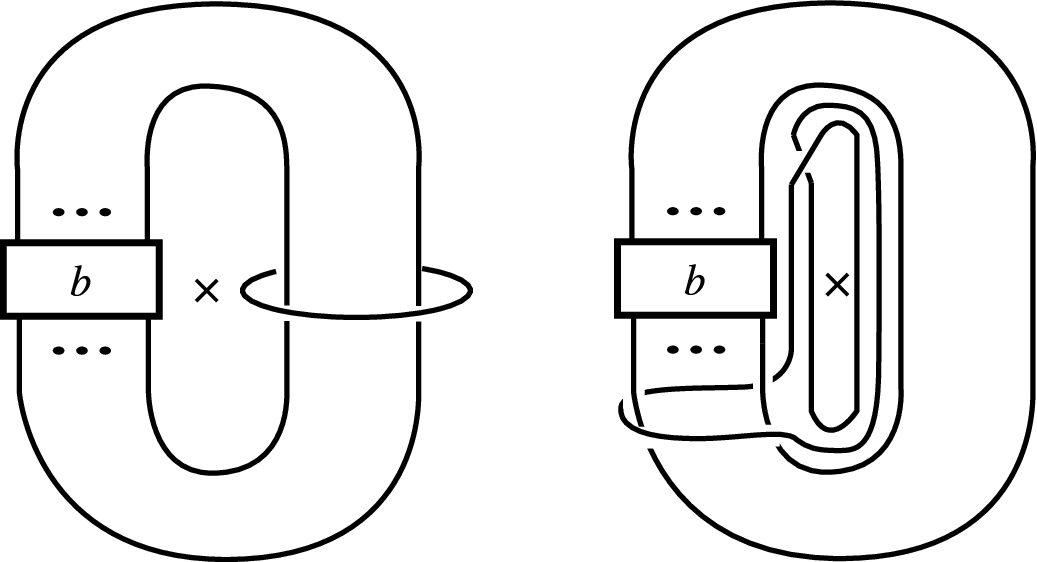
Refer to caption
Figure 14: (left) braided link β¯\overline{\beta}. (right) closed braid representing β¯\overline{\beta}.
Refer to caption
Figure 15: (left) braided link b¯\overline{b}. (center) closed 66-braid representing b¯\overline{b}. (right) closed 77-braid b′^\widehat{b^{\prime}} representing b¯\overline{b}.

Lemma 3.30 together with Corollary 3.28 implies:

Corollary 3.31.

(1)

S3∖σ1​σ22​σ3​σ4¯S^{3}\setminus\overline{\sigma_{1}\sigma_{2}^{2}\sigma_{3}\sigma_{4}} is homeomorphic to S3∖𝒞3S^{3}\setminus\mathcal{C}_{3}.

(2)

S3∖b¯S^{3}\setminus\overline{b} is homeomorphic to S3∖𝒞3S^{3}\setminus\mathcal{C}_{3}.

Proposition 3.32.

(1)

Γ⁡(σ1​σ22​σ3​σ4)\Gamma(\sigma_{1}\sigma_{2}^{2}\sigma_{3}\sigma_{4}) is the monodromy on a fiber which represents 3​α+2​β+γ3\alpha+2\beta+\gamma.

(2)

Γ⁡(b)\Gamma(b) is the monodromy on a fiber which represents 5​α+3​β+2​γ5\alpha+3\beta+2\gamma.

Proof. (1) We see that ℋ6={3​α+2​β+γ,3​α+β}\mathcal{H}_{6}=\{3\alpha+2\beta+\gamma,3\alpha+\beta\}, see the proof of Proposition 3.12. By Corollary 3.10, the monodromy for 3​α+β3\alpha+\beta permutes 44 punctures cyclically and fixes two 11 punctures. On the other hand, the monodromy for 3​α+2​β+γ3\alpha+2\beta+\gamma permutes 33 punctures cyclically, and the mapping class Γ⁡(σ1​σ22​σ3​σ4)\Gamma(\sigma_{1}\sigma_{2}^{2}\sigma_{3}\sigma_{4}) permutes 33 punctures cyclically. By Corollary 3.31(1), we complete the proof.

(2) We see that ℋ8={5​α+β,5​α+3​β+2​γ,5​α+4​β+3​γ}\mathcal{H}_{8}=\{5\alpha+\beta,5\alpha+3\beta+2\gamma,5\alpha+4\beta+3\gamma\}. The mapping class Γ⁡(b)\Gamma(b) permutes 55 punctures cyclically, 22 punctures cyclically and fixes the other 11 puncture. Among elements of ℋ8\mathcal{H}_{8}, 5​α+3​β+2​γ5\alpha+3\beta+2\gamma is the only class whose monodromy permutes 22 punctures cyclically. By Corollary 3.31(2), we complete the proof. □\Box

4 Further discussion

4.1 Pseudo-Anosov braids with small dilatation

We consider the braids Tm,p′T_{m,p}^{\prime} defined in the introduction. The braid Tm,p′T_{m,p}^{\prime} may not be pseudo-Anosov, even though Tm,pT_{m,p} is so if gcd⁡(p,m−1)=1\gcd(p,m-1)=1 (Corollary 3.28). The inequality λ⁡(Tm,p′)≤λ⁡(Tm,p)\lambda(T_{m,p}^{\prime})\leq\lambda(T_{m,p}) holds in case Tm,p′T_{m,p}^{\prime} is pseudo-Anosov. The following, which is clear by the definition of pseudo-Anosovs, says when the equality holds.

Lemma 4.1.

Suppose that gcd⁡(p,m−1)=1\gcd(p,m-1)=1. Let Φm,p\Phi_{m,p} be the pseudo-Anosov homeomorphism which represents Γ⁡(Tm,p)∈ℳ⁡(Dm)\Gamma(T_{m,p})\in\mathcal{M}(D_{m}). Corresponding to the 11st strand of Tm,pT_{m,p}, there exists a puncture, say am,pa_{m,p}, which is fixed by Φm,p\Phi_{m,p}. Suppose that the invariant foliation associated to Φm,p\Phi_{m,p} has no 11-pronged singularity at am,pa_{m,p}. Then Tm,p′T_{m,p}^{\prime} is pseudo-Anosov such that

λ⁡(Tm,p′)=λ⁡(Tm,p).\lambda(T_{m,p}^{\prime})=\lambda(T_{m,p}).

The families of braids {Tm,p′}\{T^{\prime}_{m,p}\} and {Tm,p}\{T_{m,p}\} contain examples with minimal dilatation. The following braids realize the minimal dilatation.

  • •

    T4,1′=σ1​σ2−1∈B3T_{4,1}^{\prime}=\sigma_{1}\sigma_{2}^{-1}\in B_{3}, see Matsuoka [23].

  • •

    T5,1′=σ1​σ2​σ3−1∈B4T_{5,1}^{\prime}=\sigma_{1}\sigma_{2}\sigma_{3}^{-1}\in B_{4}, see Ko-Los-Song [18] and Ham-Song [10].

  • •

    T6,2′∼σ1​σ2​σ3​σ4​σ1​σ2∈B5T_{6,2}^{\prime}\sim\sigma_{1}\sigma_{2}\sigma_{3}\sigma_{4}\sigma_{1}\sigma_{2}\in B_{5}, see Ham-Song [10].

  • •

    T6,3∼(σ2​σ1​σ2​σ1​(σ1​σ2​σ3​σ4​σ5)2)−1​Θ∈B6T_{6,3}\sim(\sigma_{2}\sigma_{1}\sigma_{2}\sigma_{1}(\sigma_{1}\sigma_{2}\sigma_{3}\sigma_{4}\sigma_{5})^{2})^{-1}\Theta\in B_{6}, see Lanneau-Thiffeault [19].

  • •

    T8,2′∼σ4−2​(σ1​σ2​σ3​σ4​σ5​σ6)2∈B7T_{8,2}^{\prime}\sim\sigma_{4}^{-2}(\sigma_{1}\sigma_{2}\sigma_{3}\sigma_{4}\sigma_{5}\sigma_{6})^{2}\in B_{7}, see Lanneau-Thiffeault [19].

  • •

    T9,5′∼σ2−1​σ1−1​(σ1​σ2​σ3​σ4​σ5​σ6​σ7)5∈B8T_{9,5}^{\prime}\sim\sigma_{2}^{-1}\sigma_{1}^{-1}(\sigma_{1}\sigma_{2}\sigma_{3}\sigma_{4}\sigma_{5}\sigma_{6}\sigma_{7})^{5}\in B_{8}, see Lanneau-Thiffeault [19].

Here b∼b′b\sim b^{\prime} means that bb is conjugate to b′b^{\prime}.

All the braids in Proposition 3.29 have been studied from the view point of their dilatations. Hironaka-Kin studied a family of braids

σ(k)=σ1σ2⋯σ2​k−2σ1σ2⋯σ2​k−4∈B2​k−1(k≥3)\sigma_{(k)}=\sigma_{1}\sigma_{2}\cdots\sigma_{2k-2}\sigma_{1}\sigma_{2}\cdots\sigma_{2k-4}\in B_{2k-1}\hskip 5.69054pt(k\geq 3)

with odd strands [12]. It is easy to see that σ(k)∼T2​k,2′\sigma_{(k)}\sim T_{2k,2}^{\prime} (cf. Proposition 3.29(1)). Each braid σ(k)∈B2​k−1\sigma_{(k)}\in B_{2k-1} has the smallest known dilatation. Venzke found a family of braids {ψn}\{\psi_{n}\} with small dilatation [31].

ψn\displaystyle\psi_{n} =\displaystyle= Ln2​σ1−1​σ2−1if​n=2​k−1​(k≥3),\displaystyle L_{n}^{2}\sigma_{1}^{-1}\sigma_{2}^{-1}\hskip 42.67912pt\mbox{if}\ n=2k-1\ (k\geq 3),
ψn\displaystyle\psi_{n} =\displaystyle= Ln2​k+1​σ1−1​σ2−1if​n=4​k​(k≥2),\displaystyle L_{n}^{2k+1}\sigma_{1}^{-1}\sigma_{2}^{-1}\hskip 28.45274pt\mbox{if}\ n=4k\ (k\geq 2),
ψn\displaystyle\psi_{n} =\displaystyle= Ln2​k+1​σ1−1​σ2−1if​n=8​k+2​(k≥1),\displaystyle L_{n}^{2k+1}\sigma_{1}^{-1}\sigma_{2}^{-1}\hskip 28.45274pt\mbox{if}\ n=8k+2\ (k\geq 1),
ψn\displaystyle\psi_{n} =\displaystyle= Ln6​k+5​σ1−1​σ2−1if​n=8​k+6​(k≥1),\displaystyle L_{n}^{6k+5}\sigma_{1}^{-1}\sigma_{2}^{-1}\hskip 28.45274pt\mbox{if}\ n=8k+6\ (k\geq 1),
ψ6\displaystyle\psi_{6} =\displaystyle= σ5​σ4​σ3​σ2​σ1​σ5​σ4​σ3​σ5​σ4,\displaystyle\sigma_{5}\sigma_{4}\sigma_{3}\sigma_{2}\sigma_{1}\sigma_{5}\sigma_{4}\sigma_{3}\sigma_{5}\sigma_{4},

where Ln=σn−1σn−2⋯σ1∈BnL_{n}=\sigma_{n-1}\sigma_{n-2}\cdots\sigma_{1}\in B_{n}. It is not hard to see that ψ2​k−1∼T2​k,2′\psi_{2k-1}\sim T_{2k,2}^{\prime}, ψ4​k∼T4​k+1,2​k+1′\psi_{4k}\sim T_{4k+1,2k+1}^{\prime}, ψ8​k+2∼T8​k+3,2​k+1′\psi_{8k+2}\sim T_{8k+3,2k+1}^{\prime}, ψ8​k+6∼T8​k+7,6​k+5′\psi_{8k+6}\sim T_{8k+7,6k+5}^{\prime}, and ψ6∼T6,2\psi_{6}\sim T_{6,2} (cf. Proposition 3.29(2)(3a)(3b)). By using Lemma 3.2 and Proposition 3.29 together with Lemma 4.1, we verify that

λ⁡(ψ2​k−1)\displaystyle\lambda(\psi_{2k-1}) =\displaystyle= λ⁡(T2​k,2′)=λ⁡(T2​k,2),\displaystyle\lambda(T^{\prime}_{2k,2})=\lambda(T_{2k,2}),
λ⁡(ψ4​k)\displaystyle\lambda(\psi_{4k}) =\displaystyle= λ⁡(T4​k+1,2​k+1′)=λ⁡(T4​k+1,2​k+1),\displaystyle\lambda(T^{\prime}_{4k+1,2k+1})=\lambda(T_{4k+1,2k+1}),
λ⁡(ψ8​k+2)\displaystyle\lambda(\psi_{8k+2}) =\displaystyle= λ⁡(T8​k+3,2​k+1′)=λ⁡(T8​k+3,2​k+1),\displaystyle\lambda(T^{\prime}_{8k+3,2k+1})=\lambda(T_{8k+3,2k+1}),
λ⁡(ψ8​k+6)\displaystyle\lambda(\psi_{8k+6}) =\displaystyle= λ⁡(T8​k+7,6​k+5′)=λ⁡(T8​k+7,6​k+5).\displaystyle\lambda(T^{\prime}_{8k+7,6k+5})=\lambda(T_{8k+7,6k+5}).

Let T(m)∈BmT_{(m)}\in B_{m} be either of the two braids realizing the minimum in Proposition 3.29. For example, T(2​k)=T2​k,2T_{(2k)}=T_{2k,2} or T2​k,2​k−3T_{2k,2k-3}. Let T(m)′∈Bm−1T_{(m)}^{\prime}\in B_{m-1} be the braid obtained from T(m)T_{(m)} by forgetting the 11st strand of T(m)T_{(m)}. By using Lemmas 4.1, 3.2 and Proposition 3.29, one has λ⁡(T(m))=λ⁡(T(m)′)\lambda(T_{(m)})=\lambda(T_{(m)}^{\prime}). By Theorem 3.3 and Proposition 3.29, we have the following.

Corollary 4.2.
(1)

λ⁡(T(2​k)′)\lambda(T^{\prime}_{(2k)}) equals the largest real root of

f(k−1,k,0)​(t)=t2​k−1−2​(tk−1+tk)+1.f_{(k-1,k,0)}(t)=t^{2k-1}-2(t^{k-1}+t^{k})+1.
(2)

λ⁡(T(4​k+1)′)\lambda(T^{\prime}_{(4k+1)}) equals the largest real root of

f(2​k−1,2​k+1,0)​(t)=t4​k−2​(t2​k−1+t2​k+1)+1.f_{(2k-1,2k+1,0)}(t)=t^{4k}-2(t^{2k-1}+t^{2k+1})+1.
(3a)

λ⁡(T(8​k+3)′)\lambda(T^{\prime}_{(8k+3)}) equals the largest real root of

f(4​k−1,4​k+3,0)​(t)=t8​k+2−2​(t4​k−1+t4​k+3)+1.f_{(4k-1,4k+3,0)}(t)=t^{8k+2}-2(t^{4k-1}+t^{4k+3})+1.
(3b)

λ⁡(T(8​k+7)′)\lambda(T^{\prime}_{(8k+7)}) equals the largest real root of

f(4​k+1,4​k+5,0)​(t)=t8​k+6−2​(t4​k+1+t4​k+5)+1.f_{(4k+1,4k+5,0)}(t)=t^{8k+6}-2(t^{4k+1}+t^{4k+5})+1.

We now discuss the monotonicity of the dilatation of braids T(m)T_{(m)}. The following proposition is a corollary of Lemma 3.17 and Proposition 3.29.

Proposition 4.3.
(1)

λ⁡(T(2​k))>λ⁡(T(2​(k+1)))\lambda(T_{(2k)})>\lambda(T_{(2(k+1))}).

(2)

λ⁡(T(4​k+1))>λ⁡(T(4​(k+1)+1))\lambda(T_{(4k+1)})>\lambda(T_{(4(k+1)+1)}).

(3a)

λ⁡(T(8​k+3))>λ⁡(T(8​(k+1)+3))\lambda(T_{(8k+3)})>\lambda(T_{(8(k+1)+3)}).

(3b)

λ⁡(T(8​k+7))>λ⁡(T(8​(k+1)+7))\lambda(T_{(8k+7)})>\lambda(T_{(8(k+1)+7)}).

One can prove the following by using the argument in the proof of Lemma 3.17.

Lemma 4.4.

λ⁡(T(2​k−1))>λ⁡(T(2​k))\lambda(T_{(2k-1)})>\lambda(T_{(2k)}).

In contrast to Lemma 4.4, it is not true that λ⁡(T(2​k))>λ⁡(T(2​k+1))\lambda(T_{(2k)})>\lambda(T_{(2k+1)}) for all kk. For example,

λ⁡(T(6))\displaystyle\lambda(T_{(6)}) <\displaystyle< λ⁡(T(7)),\displaystyle\lambda(T_{(7)}),
λ⁡(T(10))\displaystyle\lambda(T_{(10)}) <\displaystyle< λ⁡(T(11)).\displaystyle\lambda(T_{(11)}).

See the computation of λ⁡(T(m))\lambda(T_{(m)}) and ent⁡(T(m)){\mathrm{ent}}(T_{(m)}) in the following table. We shall show λ⁡(T(2​k))>λ⁡(T(2​k+1))\lambda(T_{(2k)})>\lambda(T_{(2k+1)}) is true for other cases in the next.

mm T(m)T_{(m)} λ⁡(T(m))\lambda(T_{(m)}) ent⁡(T(m)){\mathrm{ent}}(T_{(m)})
33 T3,1T_{3,1} 3.732053.73205 1.316961.31696
44 T4,2T_{4,2} or T4,1T_{4,1} 2.618032.61803 0.9624240.962424
55 T5,3T_{5,3} or T5,1T_{5,1} 2.296632.29663 0.8314430.831443
66 T6,2T_{6,2} or T6,3T_{6,3} 1.722081.72208 0.5435350.543535
77 T7,1T_{7,1} or T7,5T_{7,5} 2.081022.08102 0.7328580.732858
88 T8,2T_{8,2} or T8,5T_{8,5} 1.465571.46557 0.3822450.382245
99 T9,5T_{9,5} or T9,3T_{9,3} 1.413451.41345 0.3460310.346031
1010 T10,2T_{10,2} or T10,7T_{10,7} 1.343721.34372 0.2954420.295442
1111 T11,3T_{11,3} or T11,7T_{11,7} 1.352931.35293 0.3022710.302271
1212 T12,2T_{12,2} or T12,9T_{12,9} 1.272481.27248 0.2409650.240965
1313 T13,7T_{13,7} or T13,5T_{13,5} 1.251411.25141 0.2242730.224273
1414 T14,2T_{14,2} or T14,11T_{14,11} 1.225721.22572 0.2035260.203526
1515 T15,3T_{15,3} or T15,11T_{15,11} 1.222571.22257 0.2009580.200958
1616 T16,2T_{16,2} or T16,13T_{16,13} 1.192671.19267 0.1761910.176191
1717 T17,9T_{17,9} or T17,7T_{17,7} 1.181291.18129 0.1666090.166609
1818 T18,2T_{18,2} or T18,15T_{18,15} 1.168061.16806 0.1553450.155345
1919 T19,5T_{19,5} or T19,13T_{19,13} 1.164321.16432 0.1521360.152136
2020 T20,2T_{20,2} or T20,17T_{20,17} 1.149031.14903 0.138920.13892
2121 T21,11T_{21,11} or T21,9T_{21,9} 1.141921.14192 0.1327080.132708
2222 T22,2T_{22,2} or T22,19T_{22,19} 1.133881.13388 0.1256410.125641
2323 T23,5T_{23,5} or T23,17T_{23,17} 1.130711.13071 0.1228450.122845
2424 T24,2T_{24,2} or T24,21T_{24,21} 1.121521.12152 0.1146830.114683
2525 T25,13T_{25,13} or T25,11T_{25,11} 1.116651.11665 0.110330.11033
2626 T26,2T_{26,2} or T26,23T_{26,23} 1.111251.11125 0.1054850.105485
2727 T27,7T_{27,7} or T27,19T_{27,19} 1.108691.10869 0.1031760.103176
2828 T28,2T_{28,2} or T28,25T_{28,25} 1.102581.10258 0.09765430.0976543
2929 T29,15T_{29,15} or T29,13T_{29,13} 1.099041.09904 0.09443540.0944354
3030 T30,2T_{30,2} or T30,27T_{30,27} 1.095171.09517 0.09090690.0909069
3131 T31,7T_{31,7} or T31,23T_{31,23} 1.093091.09309 0.08900740.0890074
3232 T32,2T_{32,2} or T32,29T_{32,29} 1.088751.08875 0.08503230.0850323
3333 T33,17T_{33,17} or T33,15T_{33,15} 1.086061.08606 0.08255540.0825554
3434 T34,2T_{34,2} or T34,31T_{34,31} 1.083151.08315 0.07987140.0798714
3535 T35,9T_{35,9} or T35,25T_{35,25} 1.081441.08144 0.07829580.0782958
3636 T36,2T_{36,2} or T36,33T_{36,33} 1.078211.07821 0.07530150.0753015
3737 T37,19T_{37,19} or T37,17T_{37,17} 1.076091.07609 0.07333660.0733366
3838 T38,2T_{38,2} or T38,35T_{38,35} 1.073821.07382 0.07122650.0712265
3939 T39,9T_{39,9} or T39,29T_{39,29} 1.072411.07241 0.06990470.0699047
Lemma 4.5.

λ⁡(T(2​k))>λ⁡(T(2​k+1))\lambda(T_{(2k)})>\lambda(T_{(2k+1)}) for all k≥2k\geq 2 but k=3,5k=3,5.

The following is used for the proof of Lemma 4.5.

Lemma 4.6.

Let x′>x>1x^{\prime}>x>1 and let y′y^{\prime} be the positive number such that

XT​(x′​α+y′​β)(=x′+y′)=XT​(x​α+(x−1)​β)+1(=2​x).X_{T}(x^{\prime}\alpha+y^{\prime}\beta)(=x^{\prime}+y^{\prime})=X_{T}(x\alpha+(x-1)\beta)+1(=2x).

If λ⁡(x′​α+y′​β)<λ⁡(x​α+(x−1)​β)\lambda(x^{\prime}\alpha+y^{\prime}\beta)<\lambda(x\alpha+(x-1)\beta), then

λ⁡((x′+12)​α+(y′+12)​β)<λ⁡((x+12)​α+(x−12)​β).\lambda((x^{\prime}+\tfrac{1}{2})\alpha+(y^{\prime}+\tfrac{1}{2})\beta)<\lambda((x+\tfrac{1}{2})\alpha+(x-\tfrac{1}{2})\beta).

Proof. One can show the claim by using the same argument as in [17, Proposition 4.17]. □\Box

Proof of Lemma 4.5. One has λ⁡(3​α+β)<λ⁡(2​α+β)\lambda(3\alpha+\beta)<\lambda(2\alpha+\beta). This together with Lemma 4.6 implies that

λ⁡((2​k+1)​α+(2​k−1)​β)<λ⁡(2​k​α+(2​k−1)​β)​for all​k≥1.\lambda((2k+1)\alpha+(2k-1)\beta)<\lambda(2k\alpha+(2k-1)\beta)\hskip 5.69054pt\mbox{for\ all}\ k\geq 1.

One has another inequality λ⁡(9​α+5​β)<λ⁡(7​α+6​β)\lambda(9\alpha+5\beta)<\lambda(7\alpha+6\beta). Hence by Lemma 4.6, for all k≥2k\geq 2, one has

λ⁡((4​k+3)​α+(4​k−1)​β)\displaystyle\lambda((4k+3)\alpha+(4k-1)\beta) <\displaystyle< λ⁡((4​k+1)​α+4​k​β),\displaystyle\lambda((4k+1)\alpha+4k\beta),
λ⁡((4​k+5)​α+(4​k+1)​β)\displaystyle\lambda((4k+5)\alpha+(4k+1)\beta) <\displaystyle< λ⁡((4​k+3)​α+(4​k+2)​β).\displaystyle\lambda((4k+3)\alpha+(4k+2)\beta).

This together with Proposition 3.29 completes the proof. □\Box

As a corollary of Lemmas 4.4 and  4.5 together with the equality λ⁡(T(m))=λ⁡(T(m)′)\lambda(T_{(m)})=\lambda(T_{(m)}^{\prime}), one has:

Proposition 4.7.

(1)

λ⁡(T(2​k−1))>λ⁡(T(2​k)′)\lambda(T_{(2k-1)})>\lambda(T^{\prime}_{(2k)}) for all k≥2k\geq 2.

(2)

λ⁡(T(6))<λ⁡(T(7)′)\lambda(T_{(6)})<\lambda(T_{(7)}^{\prime}) and λ⁡(T(10))<λ⁡(T(11)′)\lambda(T_{(10)})<\lambda(T_{(11)}^{\prime}). For all k≥2k\geq 2 but k=3,5k=3,5, λ⁡(T(2​k))>λ⁡(T(2​k+1)′)\lambda(T_{(2k)})>\lambda(T^{\prime}_{(2k+1)}).

In particular, T(10)∈B10T_{(10)}\in B_{10} has smaller dilatation than the Venzke’s conjectural minimum λ⁡(ψ10)(=λ⁡(T(11)′))\lambda(\psi_{10})(=\lambda(T_{(11)}^{\prime})).

We turn to the asymptotic behavior of the normalized entropy of the braid T(m)T_{(m)}. By Theorem 3.11(1) and Proposition 3.29, we obtain the following.

Corollary 4.8.

The normalized entropy of T(m)T_{(m)} goes to the minimal normalized entropy with respect to Δ\Delta as mm goes to ∞\infty, i.e,

limm→∞ent¯​(T(m))=ent¯​(α+β)=2​log⁡(2+3).\lim_{m\to\infty}\overline{\mathrm{ent}}(T_{(m)})=\overline{\mathrm{ent}}(\alpha+\beta)=2\log(2+\sqrt{3}).

Finally, we propose a conjecture on the minimal dilatation of braids of ℓ\ell strands for ℓ≥9\ell\geq 9.

Conjecture 4.9.

(1)

The braid T(2​k)′T^{\prime}_{(2k)} realizes the minimal dilatation among (2​k−1)(2k-1)-braids for all k≥5k\geq 5.

(2)

The braid T(10)T_{(10)} realizes the minimal dilatation among 1010-braids. The braid T(2​k+1)′T^{\prime}_{(2k+1)} realizes the minimal dilatation among 2​k2k-braids for all k≥6k\geq 6.

4.2 Asymptotic behavior of entropy function

We consider asymptotic behaviors of the entropy function for a family of homology classes in Proposition 3.8.

Theorem 4.10.

Let x​α+y​β∈CΔ1x\alpha+y\beta\in C_{\Delta_{1}}.

(1)

limx,y→∞ent⁡(x​α+y​β)=0\displaystyle\lim_{x,y\to\infty}\mathrm{ent}(x\alpha+y\beta)=0.

(2)

limy→∞ent⁡(x​α+y​β)=log⁡2x.\displaystyle\lim_{y\to\infty}\mathrm{ent}(x\alpha+y\beta)=\tfrac{\log 2}{x}.

Of course, limx→∞ent⁡(x​α+y​β)=log⁡2y\displaystyle\lim_{x\to\infty}\mathrm{ent}(x\alpha+y\beta)=\tfrac{\log 2}{y} by symmetry.

Proof. (1) We may suppose that x≤yx\leq y. By [20, Theorem 3.5], we have an inequality

ent⁡(a+b)≤min⁡{ent⁡(a),ent⁡(b)}\mathrm{ent}(a+b)\leq\min\{\mathrm{ent}(a),\mathrm{ent}(b)\}

for a,b∈i​n​t​(CΔ)a,b\in int(C_{\Delta}). Hence for all ε>0\varepsilon>0 so that x−ε>0x-\varepsilon>0 and for all δ>0\delta>0,

ent⁡(x​α+(x+δ)​β)≤min⁡{ent⁡((x−ε)​α+x​β),ent⁡(ε​α+δ​β)}.\mathrm{ent}(x\alpha+(x+\delta)\beta)\leq\min\{\mathrm{ent}((x-\varepsilon)\alpha+x\beta),\mathrm{ent}(\varepsilon\alpha+\delta\beta)\}.

Notice that ent⁡(ε​α+δ​β)\mathrm{ent}(\varepsilon\alpha+\delta\beta) goes to ∞\infty as ε\varepsilon goes to 00. If one takes ε>0\varepsilon>0 sufficiently small, then one may assume that

ent⁡(x​α+(x+δ)​β)≤ent⁡((x−ε)​α+x​β).\mathrm{ent}(x\alpha+(x+\delta)\beta)\leq\mathrm{ent}((x-\varepsilon)\alpha+x\beta).

Since ent⁡(⋅)\mathrm{ent}(\cdot) is continuous, we have ent⁡(x​α+(x+δ)​β)≤ent⁡(x​α+x​β)\mathrm{ent}(x\alpha+(x+\delta)\beta)\leq\mathrm{ent}(x\alpha+x\beta). Thus,

limx→∞ent⁡(x​α+(x+δ)​β)≤limx→∞ent⁡(x​α+x​β)=limx→∞1x​ent​(α+β)=0.\lim_{x\to\infty}\mathrm{ent}(x\alpha+(x+\delta)\beta)\leq\lim_{x\to\infty}\mathrm{ent}(x\alpha+x\beta)=\lim_{x\to\infty}\tfrac{1}{x}\mathrm{ent}(\alpha+\beta)=0.

Since δ>0\delta>0 is arbitrary, the proof is completed.

(2) By Theorem 3.3, the dilatation of x​α+y​β+0​γ∈CΔ1​(ℤ)x\alpha+y\beta+0\gamma\in C_{\Delta_{1}}({\mathbb{Z}}) is the largest real root of

P⁡(tx,ty,t0)=P⁡(tx,ty,1)=ty​Rx​(t)+(Rx)∗​(t),P(t^{x},t^{y},t^{0})=P(t^{x},t^{y},1)=t^{y}R_{x}(t)+(R_{x})_{*}(t),

where Rx​(t)=tx−2R_{x}(t)=t^{x}-2. By Lemma 2.1, the largest real root of P⁡(tx,ty,1)P(t^{x},t^{y},1) converges to 21/x2^{1/x}, which is the unique real root of Rx​(t)R_{x}(t), as y→∞y\to\infty. This claim can be extended to homology classes of CΔ1​(ℚ)C_{\Delta_{1}}({\mathbb{Q}}), that is the dilatation of x​α+y​β∈CΔ1​(ℚ)x\alpha+y\beta\in C_{\Delta_{1}}({\mathbb{Q}}) converges to 21/x2^{1/x} as y→∞y\to\infty. Since the entropy function on CΔ1​(ℚ)C_{\Delta_{1}}({\mathbb{Q}}) can be extended to CΔ1C_{\Delta_{1}} uniquely, the proof is completed. □\Box

Proposition 4.11.

The entropy of (n+1)​α+n​β+(n−1)​γ∈i​n​t​(CΔ)(n+1)\alpha+n\beta+(n-1)\gamma\in int(C_{\Delta}) converges to the logarithm of the golden mean 1+52\frac{1+\sqrt{5}}{2} as nn goes to ∞\infty.

Proof. We have

P⁡(tn+1,tn,tn−1)=tn−1​(tn​(t2−t−1)+(t2−t−1)∗).P(t^{n+1},t^{n},t^{n-1})=t^{n-1}\big(t^{n}(t^{2}-t-1)+(t^{2}-t-1)_{*}\big).

If (n+1)​α+n​β+(n−1)​γ(n+1)\alpha+n\beta+(n-1)\gamma is an integral class, then its dilatation λn\lambda_{n} is the largest real root of tn​(t2−t−1)+(t2−t−1)∗t^{n}(t^{2}-t-1)+(t^{2}-t-1)_{*}. The polynomial t2−t−1t^{2}-t-1 has the real root 1+52>1\frac{1+\sqrt{5}}{2}>1. By Lemma 2.1, λn\lambda_{n} converges to 1+52\frac{1+\sqrt{5}}{2} as n∈ℕn\in{\mathbb{N}} goes to ∞\infty. Since ent⁡(⋅)\mathrm{ent}(\cdot) is continuous on i​n​t​(CΔ)int(C_{\Delta}), the proof is completed. □\Box

4.3 Relation between horseshoe braid and braid Tm,pT_{m,p}

The horseshoe map was discovered by Smale around 1960. This map is well-known to be a simple factor possessing chaotic dynamics ([26, Section 8.4.2] for example). For ϵ>0\epsilon>0, any C1+ϵC^{1+\epsilon} surface diffeomorphism with positive topological entropy “contains a horseshoe” in some iterate, see [14] for more details. This tells us that the features of the horseshoe map is universal for chaotic dynamical systems. In this section, we relate monodromies for homology classes in CΔ1​(ℤ)C_{\Delta_{1}}({\mathbb{Z}}) to the horseshoe map.

The horseshoe map H:D→DH:D\rightarrow D is an orientation preserving diffeomorphism of the disk DD defined as follows. The action of HH on the rectangle RR and two half disks S0,S1S_{0},S_{1} is given as in Figure 16. More precisely, the restriction H|RiH|_{R_{i}} for i∈{0,1}i\in\{0,1\} is an affine map such that HH contracts RiR_{i} vertically and stretches horizontally, and H|S0∪S1:S0∪S1→S0∪S1H|_{S_{0}\cup S_{1}}:S_{0}\cup S_{1}\rightarrow S_{0}\cup S_{1} is a contraction map. Then HH can be extended over the rest of DD without producing any new periodic points.

The set Ω=⋂j∈ℤHj​(R)\Omega=\displaystyle\bigcap_{j\in{\mathbb{Z}}}H^{j}(R) is invariant under HH. The map H|Ω:Ω→ΩH|_{\Omega}:\Omega\rightarrow\Omega can be described by using the symbolic dynamics as follows. We set 𝒮={0,1}ℤ\mathcal{S}=\{0,1\}^{\mathbb{Z}}, that is 𝒮\mathcal{S} is the the set of all two sided infinite sequences s=(⋯s−1s0|s1⋯)s=(\cdots s_{-1}s_{0}|s_{1}\cdots) of 00 and 11, where we put the symbol || between the 00th element and the 11st element. We introduce the metric on 𝒮\mathcal{S} as follows.

d⁡(s,t)=∑i∈ℤ|si−ti|2|i|,d(s,t)=\sum_{i\in{\mathbb{Z}}}\tfrac{|s_{i}-t_{i}|}{2^{|i|}},

where s=(⋯s−1s0|s1s2⋯)s=(\cdots s_{-1}s_{0}|s_{1}s_{2}\cdots) and t=(⋯t−1t0|t1t2⋯)t=(\cdots t_{-1}t_{0}|t_{1}t_{2}\cdots).

Theorem 4.12 (Smale).

Let 𝚜:𝒮→𝒮\mathtt{s}:\mathcal{S}\rightarrow\mathcal{S} be the shift map, i.e, 𝚜\mathtt{s} is a homeomorphism such that

𝚜(⋯s0|s1s2⋯)=(⋯s0s1|s2⋯).\displaystyle\mathtt{s}(\cdots s_{0}|s_{1}s_{2}\cdots)=(\cdots s_{0}s_{1}|s_{2}\cdots).

The restriction H|Ω:Ω→ΩH|_{\Omega}:\Omega\rightarrow\Omega is conjugate to the shift map 𝚜:𝒮→𝒮\mathtt{s}:\mathcal{S}\rightarrow\mathcal{S}. The conjugacy 𝒦:Ω→𝒮\mathcal{K}:\Omega\rightarrow\mathcal{S} is given by

𝒦⁡(x)\displaystyle\mathcal{K}(x) =\displaystyle= (⋯𝒦−1(x)𝒦0(x)|𝒦1(x)⋯),where\displaystyle(\cdots\mathcal{K}_{-1}(x)\mathcal{K}_{0}(x)|\mathcal{K}_{1}(x)\cdots),\hskip 5.69054pt\mbox{where}
𝒦j​(x)={1if Hj​(x)∈R1,0if Hj​(x)∈R0.\mathcal{K}_{j}(x)=\left\{\begin{array}[]{ll}1\hskip 8.53581pt\ \mbox{if\ }&H^{j}(x)\in R_{1},\\ 0\hskip 8.53581pt\ \mbox{if\ }&H^{j}(x)\in R_{0}.\end{array}\right.

If xx is a periodic point with the least period kk for HH, then 𝒦⁡(x)\mathcal{K}(x) is a periodic sequence. The word 𝒦0(x)𝒦1(x)⋯𝒦k−1(x)\mathcal{K}_{0}(x)\mathcal{K}_{1}(x)\cdots\mathcal{K}_{k-1}(x) is called the code for xx. Such word (modulo cyclic permutation) is said to be the code for the periodic orbit 𝒪H​(x)={x,H⁡(x),⋯,Hk−1​(x)}\mathcal{O}_{H}(x)=\{x,H(x),\cdots,H^{k-1}(x)\}.

Remark 4.13.
(1)

Theorem 4.12 asserts that there exists a one to one correspondence between the set of periodic points for H|ΩH|_{\Omega} and the set of periodic sequences in 𝒮\mathcal{S}.

(2)

By using Theorem 4.12, one can show that the set of periodic points of H|ΩH|_{\Omega} is dense on Ω\Omega.

Refer to caption
Figure 16: (1) RR, S0S_{0}, S1⊂DS_{1}\subset D. (2) horseshoe map HH. (a∗a^{*} is the image of aa under HH, for example.)

Let QQ be a set of nn points consisting of periodic orbits of H|ΩH|_{\Omega}. We take an isotopy {Ht}t∈I=[0,1]\{H_{t}\}_{t\in I=[0,1]} such that H0=H_{0}= identity map on DD and H1=HH_{1}=H. Then

b⁡(Q,{Ht}t∈I)=⋃t∈IHt​(Q)×{t}⊂D×Ib(Q;\{H_{t}\}_{t\in I})=\displaystyle\bigcup_{t\in I}H_{t}(Q)\times\{t\}\subset D\times I

is an nn-braid. This depends on the choice of the isotopy, but it is determined uniquely up to a power of the full twist Θ=(σ1⋯σn−1)n\Theta=(\sigma_{1}\cdots\sigma_{n-1})^{n}. Consider the suspension flow on the mapping torus by using a “natural” isotopy {Ht}\{H_{t}\}, see Figure 17(left). For this isotopy, we denote the braid b⁡(Q,{Ht}t∈I)b(Q;\{H_{t}\}_{t\in I}) by bQb_{Q}. By the definition of HH, one can collapse the image of the vertical lines of R0R_{0} and R1R_{1} under the isotopy to build the horseshoe template 𝒯\mathcal{T} as in Figure 17(center). (For the template theory, see [7].) In this case the template is equipped with the semiflow induced by the suspension flow. It is easy to see that there exists a one to one correspondence between the set of periodic orbits of H|ΩH|_{\Omega} and the set of periodic orbits of the semiflow on 𝒯\mathcal{T}. Each braid bQb_{Q} can be embedded in 𝒯\mathcal{T} so that the closed braid of bQb_{Q} becomes a finite union of periodic orbits of the semiflow on 𝒯\mathcal{T}. Simply, we write bQb_{Q} for the image of bQ↪𝒯b_{Q}\hookrightarrow\mathcal{T} when there exists no confusion.

Now, we define horseshoe mapping classes and horseshoe braids. Let AnA_{n} be a set of nn points which lie on the horizontal line through the origin in the round disk DD. We set an nn-punctured disk Dn=D∖AnD_{n}=D\setminus A_{n}. We say that ϕ∈ℳ⁡(Dn)\phi\in\mathcal{M}(D_{n}) is a horseshoe mapping class if there exists a set of nn points QQ consisting of periodic orbits of H|ΩH|_{\Omega} and there exists an orientation preserving homeomorphism g:D∖Q→Dng:D\setminus Q\rightarrow D_{n} such that ϕ\phi is conjugate to the mapping class [g∘H|D∖Q∘g−1]∈ℳ⁡(Dn)[g\circ H|_{D\setminus Q}\circ g^{-1}]\in\mathcal{M}(D_{n}). A braid β∈Bn\beta\in B_{n} is a horseshoe braid if the mapping class Γ⁡(β)∈ℳ⁡(Dn)\Gamma(\beta)\in\mathcal{M}(D_{n}) is a horseshoe mapping class. In other words, β\beta is a horseshoe braid if there exists an integer kk and there exists a set of nn points consisting of a finite union of periodic orbits of H|ΩH|_{\Omega}, denoted by QQ, such that β​Θk\beta\Theta^{k} is conjugate to the braid bQb_{Q}. In this case, there exists a braid γ∈Bn\gamma\in B_{n} such that γ​β​γ−1​Θk\gamma\beta\gamma^{-1}\Theta^{k} can be embedded in 𝒯\mathcal{T}. However the converse is not true. For example, the 44-braid of Figure 17(right) is not a horseshoe braid since there exists exactly one periodic orbit with the least period 22 for H|ΩH|_{\Omega} whose code is 0101. By Remark 4.13(1), one can show that a braid β\beta embedded in 𝒯\mathcal{T} (ignoring the semiflow) is a horseshoe braid if and only if no strings of the braid are parallel. (See Figure 17(right).)

Refer to caption
Figure 17: (left) suspension of horseshoe map. (center) horseshoe template 𝒯\mathcal{T}. (right) non-horseshoe 44-braid embedded in 𝒯\mathcal{T}. (In this case, two strings of the braid are parallel.)
Proposition 4.14.

Suppose that gcd⁡(p,m−1)=1\gcd(p,m-1)=1. If 1<p≤m−121<p\leq\frac{m-1}{2}, then Tm,p∈BmT_{m,p}\in B_{m} is a horseshoe braid.

Obviously, if the braid bb is written by b=c​b′b=cb^{\prime}, then bb is conjugate to b′​cb^{\prime}c. This is used for the proof of Proposition 4.14. Before proving the proposition, we first see that T12,4T_{12,4} is a horseshoe braid by using Figure 18.

Example 4.15.

The first braid of Figure 18 is a representative of T12,4T_{12,4}. We slide the last crossing in the small circle to the top, see the second braid. Then it is conjugate to the third braid of Figure 18. We repeat to slide the last crossing in the small circle of the third braid to the top. We see that it is conjugate to the fourth braid. The crossings in the large circle of the fourth braid can slide to the top, and then we see that the fourth braid is conjugate to the fifth braid which is isotopic to the sixth braid. Finally, it is easy to see that the sixth braid is conjugate to the seventh braid which can be embedded in 𝒯\mathcal{T}. (In fact, the braid σ1​σ2​σ3​σ4\sigma_{1}\sigma_{2}\sigma_{3}\sigma_{4} is a conjugacy.) Since no strings of the latter braid are parallel, one concludes that T12,4T_{12,4} is a horseshoe braid.

Refer to caption
Figure 18: conjugate braid of T12,4T_{12,4}. (1) T12,4T_{12,4}. (7) braid embedded in 𝒯\mathcal{T}.

Proof of Proposition 4.14. We consider a representative of Tm,pT_{m,p} as in the first braid of Figure 19. (See also Figure 8(left).) By using the slide technique in Example 4.15, we see that Tm,pT_{m,p} is conjugate to the second braid or the third of Figure 19. (For example, T12,4T_{12,4} is conjugate to the second type and T12,5T_{12,5} is conjugate to the third type.)

First, we show that the second braid is a horseshoe braid by using Figure 20. This braid is conjugate to the first braid of Figure 20 which is equal to the second braid of Figure 20. (See the fifth and sixth braid of Figure 18.) The second braid of Figure 20 is conjugate to the third braid in Figure 20 which can be embedded in 𝒯\mathcal{T}.

Second, we show the third braid of Figure 19 is a horseshoe braid by using Figure 21. This braid is conjugate to the first braid of Figure 21. (For example, T12,5T_{12,5} is conjugate to the third braid of Figure 21.) It is easy to see that the first braid of Figure 21 is conjugate to the second braid of Figure 21 which can be embedded in 𝒯\mathcal{T}. □\Box

Refer to caption
Figure 19: (1) Tm,pT_{m,p}. (Tm,pT_{m,p} is conjugate to either the braid drawn in (2) or the one drawn in (3).)
Refer to caption
Figure 20: conjugate braid of Tm,pT_{m,p}.
Refer to caption
Figure 21: (1,2) conjugate braid of Tm,pT_{m,p}. (3) conjugate braid of T12,5T_{12,5}.

4.4 Alternative proof of Theorem 4.10(2)

In this section, we give an alternative proof of Theorem 4.10(2).

Proof of Theorem 4.10(2). By Proposition 3.26, we have seen that Tm,1T_{m,1} represents the monodromy of (m−2)​α+β∈CΔ1​(ℤ)(m-2)\alpha+\beta\in C_{\Delta_{1}}({\mathbb{Z}}). For the proof, it is enough to show that

limm(∈ℕ)→∞ent⁡((m−2)​α+β)=log⁡2.\lim_{m(\in{\mathbb{N}})\to\infty}\mathrm{ent}((m-2)\alpha+\beta)=\log 2. (4.1)

The reason is as follows. The equality in (4.1) implies that

limx→∞ent⁡(x​α+β)=log⁡2\displaystyle\lim_{x\to\infty}\mathrm{ent}(x\alpha+\beta)=\log 2

by the continuity of ent⁡(⋅)\mathrm{ent}(\cdot). Therefore

ent⁡(x​α+y​β)=1y​ent​(xy​α+β)→log⁡2y​as ​x→∞.\mathrm{ent}(x\alpha+y\beta)=\tfrac{1}{y}\mathrm{ent}(\tfrac{x}{y}\alpha+\beta)\to\tfrac{\log 2}{y}\hskip 5.69054pt\mbox{as\ }x\to\infty.

Now we show (4.1). Let β(m1,m2,⋯,mk+1)\beta_{(m_{1},m_{2},\cdots,m_{k+1})} be a family of braids depicted in Figure 22 for each integer k≥1k\geq 1 and each integer mi≥1m_{i}\geq 1. By [16, Theorem 1.2], these braids are all pseudo-Anosov and the dilatation of β(m1,⋯,mk+1)\beta_{(m_{1},\cdots,m_{k+1})} is the largest real root of the Salem-Boyd polynomial

tmk+1​R(m1,⋯,mk)​(t)+(−1)k+1​R(m1,⋯,mk)∗​(t),t^{m_{k+1}}R_{(m_{1},\cdots,m_{k})}(t)+(-1)^{k+1}{R_{(m_{1},\cdots,m_{k})}}_{*}(t),

where R(m1,⋯,mi)​(t)R_{(m_{1},\cdots,m_{i})}(t) is given inductively as follows: For 2≤i≤k2\leq i\leq k,

R(m1)​(t)\displaystyle R_{(m_{1})}(t) =\displaystyle= tm1+1​(t−1)−2​t,\displaystyle t^{m_{1}+1}(t-1)-2t,
R(m1,⋯,mi)​(t)\displaystyle R_{(m_{1},\cdots,m_{i})}(t) =\displaystyle= tmi​(t−1)​R(m1,⋯,mi−1)​(t)+(−1)i​2​t​R(m1,⋯,mi−1)∗​(t).\displaystyle t^{m_{i}}(t-1)R_{(m_{1},\cdots,m_{i-1})}(t)+(-1)^{i}2t{R_{(m_{1},\cdots,m_{i-1})}}_{*}(t).

In particular, the dilatation of β(1,m−3)=σ1−1σ2σ3⋯σm−2∈Bm−1\beta_{(1,m-3)}=\sigma_{1}^{-1}\sigma_{2}\sigma_{3}\cdots\sigma_{m-2}\in B_{m-1} is the largest root of

tm−2​R(1)​(t)+(R(1))∗​(t),t^{m-2}R_{(1)}(t)+(R_{(1)})_{*}(t), (4.2)

where R(1)​(t)=t⁡(t+1)​(t−2)R_{(1)}(t)=t(t+1)(t-2). By Lemma 2.1, the dilatation of β(1,m−3)\beta_{(1,m-3)} converges to 22 as m→∞m\to\infty. The polynomial (4.2) comes from the graph map shown in Figure 23(center). This is the induced graph map for β(1,m−3)∈Bm−1\beta_{(1,m-3)}\in B_{m-1}. The polynomial (4.2) is the characteristic polynomial of the transition matrix for the graph map. The smoothing of the graph gives rise to the train track associated to β(1,m−3)\beta_{(1,m-3)} (Figure 23(right)). Since the train track contains an (m−2)(m-2)-gon, a pseudo-Anosov homeomorphism Φβ(1,m−3)\Phi_{\beta_{(1,m-3)}} which represents the mapping class β(1,m−3)\beta_{(1,m-3)} has an (m−2)(m-2)-pronged singularity, say pp, in the interior of the punctured disk. By puncturing the point pp, one obtains a pseudo-Anosov homeomorphism Φ^β(1,m−3)\widehat{\Phi}_{\beta_{(1,m-3)}}. It is easy to see that the mapping class [Φ^β(1,m−3)][\widehat{\Phi}_{\beta_{(1,m-3)}}] is given by

β^(1,m−3)=σ1−1σ2σ3⋯σm−2σm−12∈Bm\widehat{\beta}_{(1,m-3)}=\sigma_{1}^{-1}\sigma_{2}\sigma_{3}\cdots\sigma_{m-2}\sigma_{m-1}^{2}\in B_{m}

with the same dilatation as β(1,m−3)\beta_{(1,m-3)}. Since β^(1,m−3)\widehat{\beta}_{(1,m-3)} is conjugate to the braid Tm,1T_{m,1}, the dilatation λ⁡(Tm,1)\lambda(T_{m,1}) converges to 22 as mm goes to ∞\infty. This completes the proof. □\Box

Refer to caption
Figure 22: (left) β(m1,m2,⋯,mk+1)\beta_{(m_{1},m_{2},\cdots,m_{k+1})}. (center) β(1,4)\beta_{(1,4)}. (right) β^(1,m−3)\widehat{\beta}_{(1,m-3)}.
Refer to caption
Figure 23: (left) transition of peripheral edge. (center) graph map. (right) train track.

References

  • [1] J. W. Aaber and N. M. Dunfield, Closed surface bundles of least volume, preprint, arXiv:1002.3423
  • [2] M. Bestvina and M. Handel, Train-tracks for surface homeomorphisms, Topology 34 (1994), 109-140.
  • [3] E. Elrifai and H. Morton, Algorithm for positive braids, The Quarterly Journal of Mathematics. Oxford. Second Series 45 (1994), 479-497.
  • [4] B. Farb, C. J. Leininger and D. Margalit, Small dilatation pseudo-Anosovs and 33-manifolds, preprint, arXiv:0905.0219
  • [5] A. Fathi, F. Laudenbach and V. Poenaru, Travaux de Thurston sur les surfaces, Asterisque, 66-67, Société Mathématique de France, Paris (1979).
  • [6] D. Fried, Flow equivalence, hyperbolic systems and a new zeta function for flows, Commentarii Mathematici Helvetici. 57 (1982), 237-259.
  • [7] R. Ghrist, P. Holmes, and M. Sullivan, Knots and Links in Three-Dimensional Flows, Lecture Notes in Mathematics 1654, Springer-Verlag (1997).
  • [8] J. González-Meneses, http://personal.us.es/meneses/
  • [9] C. Gordon, Small surfaces and Dehn filling, Geometry & Topology Monographs 2 (1999), 177-199.
  • [10] J. Y. Ham and W. T. Song, The minimum dilatation of pseudo-Anosov 55-braids, Experimental Mathematics 16 (2007), 167-179.
  • [11] E. Hironaka, Small dilatation pseudo-Anosov mapping classes coming from the simplest hyperbolic braid, preprint, arXiv:0909.4517
  • [12] E. Hironaka and E. Kin, A family of pseudo-Anosov braids with small dilatation, Algebraic and geometric topology 6 (2006), 699-738.
  • [13] N. V. Ivanov, Coefficients of expansion of pseudo-Anosov homeomorphisms, Zap. Nauchu. Sem. Leningrad. Otdel. Mat. Inst. Steklov. (LOMI), 167 (1988), Issled. Topol. 6, 111-116, 191, translation in Journal of Soviet Mathematics, 52 (1990), 2819-2822.
  • [14] A. Katok, Lyapunov exponents, entropy and periodic orbits for diffeomorphisms, Institut des Hautes Études Scientifiques. Publications Mathématiques 51 (1980), 137-174.
  • [15] E. Kin, S. Kojima and M. Takasawa, Entropy versus volume for pseudo-Anosovs, Experimental Mathematics 18 (2009), 397-407.
  • [16] E. Kin and M. Takasawa, An asymptotic behavior of the dilatation for a family of pseudo-Anosov braids, Kodai Mathematical Journal 31 (2008), 92-112.
  • [17] E. Kin and M. Takasawa, Pseudo-Anosovs on closed surfaces having small entropy and the Whitehead sister link exterior, preprint, arXiv:1003.0545
  • [18] K. H.  Ko, J. Los and W. T.  Song, Entropies of Braids, Journal of Knot Theory and its Ramifications 11 (2002), 647-666.
  • [19] E. Lanneau and J. L.  Thiffeault, On the minimum dilatation of braids on the punctured disc, preprint, arXiv:1004.5344
  • [20] D. Long and U. Oertel, Hyperbolic surface bundles over the circle, Progress in knot theory and related topics, Travaux en Course 56, Hermann, Paris (1997), 121-142.
  • [21] B. Martelli and C. Petronio, Dehn filling of the “magic” 33-manifold, Communications in Analysis and Geometry 14 (2006), 969-1026.
  • [22] S. Matsumoto, Topological entropy and Thurston’s norm of atoroidal surface bundles over the circle, Journal of the Faculty of Science, University of Tokyo, Section IA. Mathematics 34 (1987), 763-778.
  • [23] T. Matsuoka, Braids of periodic points and 22-dimensional analogue of Shorkovskii’s ordering, Dynamical systems and Nonlinear Oscillations (Ed. G. Ikegami), World Scientific Press (1986), 58-72.
  • [24] C. McMullen, Polynomial invariants for fibered 33-manifolds and Teichmüler geodesic for foliations, Annales Scientifiques de l’École Normale Supérieure. Quatrième Série 33 (2000), 519-560.
  • [25] U. Oertel, Affine laminations and their stretch factors, Pacific Journal of Mathematics 182 (1998), 303-328.
  • [26] C. Robinson, Dynamical Systems, Stability, Symbolic Dynamics, and Chaos (second edition), CRC Press, Ann Arbor, MI (1995).
  • [27] W. Thurston, The geometry and topology of 33-manifolds, Lecture Notes, Princeton University (1979).
  • [28] W. Thurston, A norm of the homology of 33-manifolds, Memoirs of the American Mathematical Society 339 (1986), 99-130.
  • [29] W. Thurston, On the geometry and dynamics of diffeomorphisms of surfaces, Bulletin of the American Mathematical Society 19 (1988), 417-431.
  • [30] W. Thurston, Hyperbolic structures on 3-manifolds II: Surface groups and 3-manifolds which fiber over the circle, preprint, arXiv:math/9801045
  • [31] R. Venzke, Braid forcing, hyperbolic geometry, and pseudo-Anosov sequences of low entropy, PhD thesis, California Institute of Technology (2008), available at http://etd.caltech.edu/etd/available/etd-05292008-085545/
  • [32] P. Walters, An Introduction to Ergodic Theory, Springer-Verlag (1982).

Department of Mathematical and Computing Sciences, Tokyo Institute of Technology, Ohokayama, Meguro Tokyo 152-8552 Japan
E-mail address: kin@is.titech.ac.jp

Department of Mathematical and Computing Sciences, Tokyo Institute of Technology, Ohokayama, Meguro Tokyo 152-8552 Japan
E-mail address: takasawa@is.titech.ac.jp