HIP-2008-38/TH
December, 2008
Vortices, Q-balls and Domain Walls
on Dielectric M2-branes
Masato Arai†aa a arai(at)sogang.ac.kr, Claus Montonen‡bb b claus.montonen(at)helsinki.fi and Shin Sasaki‡cc c shin.sasaki(at)helsinki.fi
†Center for Quantum Spacetime (CQUeST), Sogang University,
Shinsu-dong 1, Mapo-gu, Seoul 121-742, Korea
‡Department of Physics,
University of Helsinki
Helsinki Institute of Physics,
P.O.Box 64, FIN-00014, Finland
We study BPS solitons in Chern-Simons-matter theory deformed by an F-term mass. The F-term mass generically breaks supersymmetry down to . At vacua, M2-branes are polarized into a fuzzy forming a spherical M5-brane with topology . The polarization is interpreted as Myers’ dielectric effect caused by an anti-self-dual 4-form flux in the eleven-dimensional supergravity. Assuming a polarized M2-brane configuration, the model effectively reduces to the well-known abelian Chern-Simons-Higgs model studied in detail by Jackiw-Lee-Weinberg. We find that the potential for the fuzzy radius agrees with the one calculated from the M5-brane point of view at large . This effective model admits not only BPS topological vortex and domain wall solutions but also non-topological solitons that keep 1/4 of the manifest supersymmetry. We also comment on the reduction of our configuration to ten dimensions.
1 Introduction
No one doubts that understanding various aspects of low-energy effective theory of M2-branes enables us to uncover mysterious properties of M-theory and non-perturbative physics of string theories. Recently, Bagger, Lambert and Gustavsson proposed a three-dimensional superconformal Chern-Simons model based a novel 3-algebra (BLG model) [1, 2]. This model has been expected to describe the low energy effective theory of two coincident M2-branes in eleven dimensions. However, it seemed difficult to generalize their model to the case of arbitrary number of M2-branes.
Meanwhile, Aharony-Bergman-Jafferis-Maldacena proposed a three-dimensional Chern-Simons-matter theory with level (ABJM model) which may be regarded as the low-energy effective theory of coincident M2-branes probing orbifold [3]. The model consists of gauge fields , four complex scalars in the (anti) bi-fundamental representation of the gauge group, and their superpartners. The model is believed to be a dual description of M-theory on .
After the proposal by Aharony-Bergman-Jafferis-Maldacena, a lot of works on the effective theory of interacting multiple membranes have been studied. Among them, classical solutions in the three-dimensional M2-brane world-volume theory attracted much attention since these solutions can be interpreted as various configurations of branes existing in the eleven-dimensional M-theory. In [4], a BPS fuzzy funnel configuration that represents an M5-brane intersecting with multiple M2-branes was found11 1 A similar analysis in the BLG model has been performed in [5].. A domain wall solution that interpolates between fuzzy and trivial vacua was found [6] in the mass deformed ABJM model that has maximal supersymmetry. These solutions preserve half of supersymmetry. On the other hand, time evolutions of fuzzy and M5/anti-M5 configurations that are generically non-BPS were investigated in [7]. These results provide some evidence that the ABJM model gives a correct description of the dynamics of multiple membranes.
On the other hand, in [8], dual theory of M2-branes with reduced supersymmetry was investigated following the prescription studied by Polchinski-Strassler [9]. The author of [8] proposed a mass deformation of multiple membrane theory with world-volume supersymmetry and studied a probe M5-brane in the presence of anti-self-dual 4-form flux in the eleven-dimensional supergravity. The vacua are spherical M5-branes with topology sharing three dimensions with M2-branes. He conjectured that there exists BPS domain walls that interpolate between various vacua in the model. However, the correct description of the mass deformed multiple M2-brane theory was not known at that time.
In this paper, we study the ABJM model deformed by an F-term mass which was first introduced in [10]. The F-term mass generically breaks supersymmetry down to preserving global symmetry of and the resulting model is identified with the model studied in [8]. We find that a vacuum configuration of the model is a fuzzy . We see that the radius of the sphere derived here coincides with the one obtained in [8] at large- identifying our vacuum as a spherical M5-brane with topology . From the viewpoint of the M2-brane world-volume theory, this is nothing but Myers’ dielectric effect [11] caused by eleven-dimensional supergravity flux . We also see that reducible configurations found in [10] are identified with a set of fuzzy shells.
In the latter half of this paper, we study various classes of BPS configurations with polarized M2-brane geometry in the mass deformed ABJM model. Assuming a polarized M2-brane configuration, we find that the Hamiltonian effectively reduces to that of the well-known abelian Chern-Simons-Higgs system with sixth-power potential studied in detail by Jackiw-Lee-Weinberg [12]. It has been known that this model exhibits an supersymmetry in three dimensions [13] and admits BPS topological vortices and domain walls. In addition, there exists non-topological soliton solutions [14] and a BPS supertube solution [15]. We find that the potential for the radius in the effective Hamiltonian has the same structure as found in [8]. Since the configurations corresponding to the BPS solutions can exist only in the case of non-zero , these solutions are supported against collapse by the non-zero background flux realizing a generalization of the Myers effect.
The organization of this paper is as follows. In section 2, we introduce the ABJM model deformed by the F-term mass. Equations of motion and on-shell supersymmetry transformations are derived. In section 3, we study the vacuum structure of the model. We compare the radius of the fuzzy with the one found in [8] at large- finding agreement between them. In section 4, assuming an ansatz, we derive the effective Hamiltonian that reduces to the abelian Chern-Simons-Higgs model studied in [12, 16]. The non-abelian property of fields is totally encoded into the “BPS matrices” first constructed in [10]. We then perform the Bogomol’nyi completion in the effective Hamiltonian combining the kinetic and potential terms and derive the BPS equations. The consistency between these BPS equations and the full equations of motion, as well as the number of preserved supersymmetries are discussed. In section 5, parts of the exact and numerical results of the BPS solutions are discussed. Possible interpretations of these solutions in terms of eleven-dimensional M-theory are briefly discussed in this section. Section 6 is devoted to conclusions and discussions. In appendix A, the explicit form of the BPS matrices is presented. The superfield formulation of the ABJM model can be found in appendix B. The effective Lagrangian including fermion parts on the polarized M2-branes can be found in appendix C.
2 The ABJM model
The ABJM model [3] is a (2+1)-dimensional superconformal Chern-Simons-Higgs model of level with gauge symmetry. The model is expected to describe the low energy world-volume theory of coincident M2-branes probing . We employ the notation and convention of [17] but with a different normalization of the gauge generators such that . The bosonic part of the massless ABJM action is
| (1) |
where each term is given by
| (2) | |||||
| (3) |
| (4) | |||||
Here , are gauge fields, are complex scalar fields in the bi-fundamental representation. The world-volume metric is . The gauge covariant derivative is
| (5) |
The gauge field strength is defined as
| (6) |
and similarly for . The common charge is fixed to . The model exhibits a manifest global symmetry. Under the each s, transform independently in the fundamental representation. Apart from this manifest symmetry, there is an symmetry under which the fields (and ) transform as a doublet. It was discussed in [3] that the global symmetry is combined with the and enhanced to . Therefore, for , the model has supersymmetry. We consider a trivial embedding of the world-volume in the space-time. Namely, the world-volume coordinates are identified with the space-time coordinates . The four complex scalars represent the transverse displacement of the M2-branes along eight directions . The orbifolding symmetry act as . The superfield formalism of the model can be found in Appendix B.
The Gauss’ law constraint comes from the equation of motion for the gauge fields,
| (7) | |||
| (8) |
The Noether current and charge corresponding to the following gauge transformation (which we call baryonic )
| (9) |
are derived as
| (10) | |||
| (11) |
Let us consider massive deformations of the model. There are two kinds of massive deformations: F- and D-term deformations [10]22 2 See also [18] for massive deformations with reduced supersymmetries.. Here we focus on the F-term mass deformation. The superpotential is given by
| (12) |
where
| (13) |
is the original superpotential in the massless ABJM model [17] and 33 3 Note that its “conjugate” part is given by . The minus sign in front of comes from the extra minus sign of the components in a “conjugated” superfield [17]. See Appendix B.
| (14) |
is a mass term which breaks the global symmetry down to and keeps manifest the supersymmetry. This is different from the D-term mass deformation which keeps the manifest symmetry and preserves maximal supersymmetry [10]. Here the transformation swaps and . It is easy to derive the equation of motion for the scalar fields. The full equation of motion for is
| (15) |
The equation of motion for is obtained by replacing with in the above expression.
For later convenience, we derive the Hamiltonian of the model. The Chern-Simons part gives a vanishing contribution because it is a topological quantity. However, the gauge fields enter in the Hamiltonian through the covariant derivative. The result is
| (16) |
where the potential part is
| (17) | |||||
| (18) | |||||
As we mentioned, the model exhibits at least manifest supersymmetry. It can be shown that the model is invariant under the following (on-shell) supersymmetry,
| (20) | |||
| (21) | |||
| (22) | |||
| (23) | |||
| (24) | |||
| (25) |
where are fermionic partners, and are auxiliary fields whose equations of motion are given in (117)-(121) in appendix B. The supersymmetric transformation is achieved by the operator where is a supercharge and is a two component complex spinor.
3 Vacua as dielectric M2-branes
In this section, we discuss the physical meaning of our F-term deformation and investigate the vacuum structure of the model. For the massless ABJM model, there is a dual description as M-theory on at large- 44 4 We here focus on the sector where the orbifolding by becomes trivial. However, we expect that the results in this section hold even for the case.. We can perturb the side by turning on a non-trivial supergravity flux which causes additional terms on the dual M2-brane side. Indeed, in [8], Bena considered a mass perturbation of the theory of coincident M2-branes. Its fermionic part is given by
| (26) |
Here are complexified Majorana fermions living on the M2-branes. The mass term keeps at least supersymmetry of the maximal supersymmetry. The mass terms for the scalar fields break symmetry down to . We will discuss this issue of global symmetry a little bit in detail later. The author of [8] conjectured that the deformed model is given by a superpotential of the form
| (27) |
where are chiral superfields whose lowest components are complex scalars representing fluctuations along transverse directions to the M2-brane world-volume. The non-zero mass parameter on the M2-brane side was identified with non-trivial anti-self-dual constant 4-form flux on the supergravity side via /CFT duality. The 4-form flux has a non-trivial value in the directions transverse to the M2-branes. The “(anti) self-dual” means that the flux satisfies
| (28) |
where is the eight-dimensional epsilon tensor and indices run from 3 to 10.
One may imagine that the M2-branes are polarized due to the background flux forming another higher dimensional brane in eleven-dimensions. The most natural candidate of this higher dimensional brane is an M5-brane. Indeed, the vacuum structure of this deformed model was studied through an examination of a probe M5-brane with -units of M2-brane charge in the perturbed by the flux. For the case of four equal masses, which is our concern here, the supersymmetric vacuum is a configuration of an M5-brane with geometry . Its directions are shared with the M2-branes while other three-dimensions are wrapped on an inside the . The radius of the was derived by evaluating the M5-brane action via the Pasti-Sorokin-Tonin and Perry-Schwarz approaches [19, 20]. Its “potential” term at large- is [8]
| (29) |
where and is the eleven-dimensional Planck mass. Here we have added the overall M5-brane tension , which was ignored in [8], and we have restricted ourselves to the 3456 plane in the 3-7, 4-8, 5-9, 6-10 planes using rotations [8]. From the result (29), we find a supersymmetric vacuum
| (30) |
Apart from the non-zero radius, there is also a trivial vacuum . Therefore there should exist a domain wall solution which interpolates between these vacua. It was conjectured that the tension of a domain wall is
| (31) |
The above situation can be extended to the case that the M2-branes are uniformly distributed on more than one 3-sphere, with M5-brane charges. The potential felt by a probe M5-brane with M2-brane charges is still written by (29), but with a different radius and M2-brane charges . Its form is given by (once again restricting to the 3456 plane),
| (32) |
where . Therefore the ground states form M2-brane 3-sphere shells with radius .
With these results in mind, let us return to our model. The ABJM model deformed by the F-term mass is given by the superpotential (12). This is just the superpotential (27) conjectured in [8]. Its fermionic part is nothing but the equation (26) via the identification
| (33) |
The mass perturbation part (14) keeps which is a subgroup of the expected R-symmetry group . However, we remind the fact that for the massless ABJM model, the global symmetry does not commute with the , they combine giving an symmetry. This mechanism of symmetry enhancement would be true even for our case. Although it is not manifest here, the remaining global symmetry would be combined with generating .
The supersymmetric vacuum of our model can be obtained as follows [10]. Assuming a configuration
| (34) |
the condition is automatically satisfied. Here are BPS matrices [10] presented in appendix A. The F-term condition
| (35) |
yields the following vacua
| (36) |
where is a trivial vacuum. At the vacuum corresponding to , the gauge symmetry is broken to . One of these s is the “baryonic ”, eq. (9), and the other one being an independent rotation of a degree of complexity freedom which decouples when the ansatz (34) is used. To see the physical meaning of solution, let us define the following combinations of the transverse fluctuation modes
| (37) |
Due to the ansatz , only is non-zero. Therefore half of the eight transverse degrees of freedom is now dropped and this configuration is nothing but a fuzzy with radius
| (38) |
Here is a tension of an M2-brane. We have used the relation that the -brane tension in eleven-dimensions is given by . This result coincides with the equation (30) obtained from the dual M5-brane description. Therefore the vacuum configuration (36) is interpreted as polarized M2-branes caused by the background flux with its VEV . This is just an M-theory realization of Myers’ dielectric effect [11].
Because the model admits vacua and in each sector they have different values of the superpotential, there is a domain wall solution that interpolates between them. Indeed, it is easy to find such a solution with vanishing gauge fields. The Bogomol’nyi completion of the energy density for the configuration with vanishing gauge fields is
| (39) | |||||
where the surface term is
| (40) | |||||
The BPS equations are obtained by requiring that and the vanishing condition inside the absolute values in the equation (39). A solution to these equations is given by
| (41) |
which also satisfies the Gauss’ law (7) and (8). This solution is just the one first found in [6], but they obtained it in the D-term deformed theory.
We can see that the solution (41) keeps a half of supersymmetry specified by
| (42) |
while the one in [6] keeps half of the maximal supersymmetry. The tension of the domain wall is evaluated as
| (43) |
This agrees with the result (31).
Before going to the next section, we would like to consider the reducible vacuum solutions discussed in [10]. Because the BPS matrices for any partition of do satisfy the vacuum condition, there is a set of reducible solutions that is obtained by replacing by
Here satisfy and are the BPS matrices in an dimensional representation. We will see in a later section that these vacua correspond to a set of fuzzy shells with different values of the radius and that the potential is written as in (32).
It is possible to capture the brane configuration corresponding to a domain wall interpolating between one of the reducible vacua constructed, for example, by at and the irreducible vacuum with dimension at . It is easy to show that the large- behavior of its tension is the same as in (43). Following the discussion in [9, 8], in the region , the configuration is interpreted as an M5-brane extending in the directions and wrapping an with M2-brane charge while in the region , it is an M5-brane extending along the same directions and wrapping an with charge . They are generically both bent and meet at a point . Because of charge conservation, another new M5-brane with charge should exist at that point. This is a kind of brane junction. Because all M5-branes meet at a point, one direction should be supplemented for the new M5-brane. This is possible if we consider a ball instead of a sphere . Therefore the other new M5-brane is extending along the directions and filling a four-ball with its surface . A schematic picture is given in Fig. 1.

4 Effective Hamiltonian and BPS equations
In this section, motivated by the discussion in the previous section on the spherical M5-brane at the vacuum, we study the effective Hamiltonian for the configuration of polarized M2-branes. We will see that the potential for the radius of this configuration coincides with (29) at large . Consider an ansatz
| (48) |
where are the BPS matrices. This configuration represents the M2-branes polarized into a fuzzy . The physical radius of the fuzzy is given by
| (49) |
Under the ansatz, the covariant derivative becomes
| (50) |
while the gauge field strength satisfies
| (51) | |||||
| (52) |
The equation of motions for and reduce to the following equation for ,
| (53) |
For the case of the ansatz (48), we have
| (54) |
Therefore, from the equation (16), the effective Hamiltonian for the polarized M2-branes is given by
| (55) |
This is nothing but the Hamiltonian for an abelian Chern-Simons Higgs model studied in [12, 16, 21] and [15]. Note that all the non-abelian structures in the model have been encoded into the overall factor by the help of the BPS matrices. Although the gauge symmetry has been effectively reduced to the abelian symmetry, the Hamiltonian still describes M2-branes.
It is known that the abelian Chern-Simons-Higgs model with the potential given in (55) exhibits a three-dimensional supersymmetry [13] and admits various class of BPS soliton solutions. See appendix C for the full structure of the Lagrangian including fermion parts. Following the analysis in [15], we find a Bogomol’nyi completion of the energy,
| (56) | |||||
where we have used the gauge field equation of motion. Therefore we have an energy bound
| (57) |
Here the following quantities have been defined,
| (58) | |||
| (59) | |||
| (60) | |||
| (61) |
Here are (time integrals of) the magnetic flux, the angular momentum, the linear momentum along direction, the tension of a domain wall. The energy bound (57) is saturated when the angle satisfies the following condition
| (62) |
The baryonic charge (11) for our ansatz is evaluated as
| (63) |
Using the equation of motion for the gauge field, we have the relation
| (64) |
The Noether charge is proportional to the magnetic flux. This is a specific property of Chern-Simons solitons. From the Bogomol’nyi completed form of the Hamiltonian (56), we obtain the BPS equations,
| (65) | |||
| (66) |
Requiring that the supersymmetry transformations (22) and (23) of the fermionic fields vanish combined with these BPS equations yields the following conditions,
| (67) | |||
| (68) |
where are the three-dimensional -matrices given in appendix B. This tells us that the BPS equations retain a quarter of the supersymmetry, specified by the effective supercharge (in the case )
| (69) |
One should be careful about the above procedure deriving the BPS equations (65), (66). We first assumed an ansatz and derived the effective Hamiltonian (56) which is valid only for the special configuration (48). There is a possibility that the BPS equations are not consistent with the original equations of motion. Let us check this issue. Once the equations (65), (66) are satisfied, we have
| (70) |
This is the equation of motion (15) for for the ansatz (48). Therefore the BPS equations (65), (66) are consistent with the full (second order) equations of motion for .
Note that in terms of the physical fuzzy radius , the potential term in the equation (56) becomes
| (71) |
At large , this gives
| (72) |
where we have used . After a trivial rescaling of , the result agrees with the potential (29) evaluated from the spherical M5-brane. Once we consider the reducible ansatz , the potential is a sum of the each sectors, i.e., it is given by
| (73) |
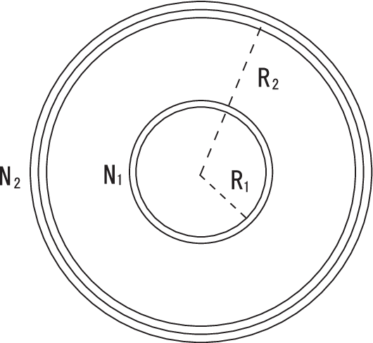
This has the same form of the potential for the M2-branes distributed over a 3-sphere (32) giving a 3-sphere shells of M2-branes [8]. Therefore the reducible configuration can be interpreted as a set of M2-branes polarized into fuzzy spheres with radii . See Fig. 2 for a schematic picture.
A comment on this reducible configuration is in order. We have ignored off-block-diagonal parts of to derive the equation (73). The result is the sum of the potentials for the radii inside stack of M2-branes without any interactions among each stacks. Once we turn on the off-block-diagonal parts, it represents interactions among each stack of M2-branes and hence, in the dual picture, interactions among M5-branes.
5 Solutions
In this section, we explore solutions for the BPS equations (65), (66). Since it is difficult to find solutions for general cases, we focus on the simplest situations. Let us first consider the static case. In this case must vanish and the energy bound is given by and . The BPS equations reduce to
| (74) | |||
| (75) |
This is nothing but the equation (14) in [16]. Following [12], we now assume an ansatz
| (76) | |||||
| (77) |
where are polar coordinates in the M2-brane world-volume and is an integer. The BPS equations (74), (75) reduce to
| (78) | |||||
| (79) |
Here the prime stands for the differentiation with respect to . Requiring and to be non-singular at the origin, we obtain boundary conditions
| (80) |
On the other hand, the condition of finite energy is requiring that the scalar field settles down to its vacuum configuration at infinity, namely,
From the equations (78), (79), we obtain
| (84) |
When is small, the term can be neglected and we can find an explicit solution [12]. That is given by
| (85) |
Here are arbitrary constants. The energy density for the ansatz (76) and (77) is given by
| (86) | |||||
| (87) |
The magnetic charges and angular momentum are also readily written down as
| (88) | |||
| (89) |
and and . Here we have defined . Considering the boundary conditions (80) and (5), (88) and (89) become
| (90) |
where and . In the following analysis, we consider the case , which corresponds to choosing the plus sign in (76) and (77). We will also see that for all the cases we will discuss below. Because the detailed study of the global structure of these solutions has been performed in [12], we just briefly describe the solutions according to the boundary conditions.
5.1 Vortices
First consider the case of the boundary condition . For the case, the only solution is the vacuum configuration, and . Thus it is just the spherical M5-brane discussed in section 3. For the case, a topologically non-trivial configuration appears, which connects the boundaries and . They are vortex solutions. Although, no explicit solutions of the equation for this boundary condition is not known, it is possible to solve it numerically. In Fig. 3, we plot and for the solution and its corresponding energy density. We also show the magnetic flux density in Fig. 4. We can see that the topological charge is given by the magnetic flux . As can be seen in Fig. 3, in almost all of the region of the M2-brane world-volume, the configuration represents the vacuum fuzzy discussed in section 3 but at the origin, there is a “dimple” inside which the full supersymmetry is recovered.
5.2 Q-balls
Next we consider the case and . In this case, the scalar function approaches the trivial vacuum and therefore all configurations are topologically trivial. The gauge field part starts from the boundary and approaches some value which characterizes the value of magnetic flux . The magnetic flux is given by the Noether charge through the relation (64). This kind of solution is called a Q-ball . This is a lump-like object localized on a ring which surrounds the origin. Around the origin, the fuzzy has non-zero radius but the full supersymmetry is generically broken there. This is because the value of at the origin need not to be the value in the vacuum. The situation is similar at infinity where the fuzzy sphere collapses into zero size but the gauge field has non-zero value. The plots of the solution and corresponding energy density are shown in Fig. 5. The behavior of the magnetic flux is shown in Fig. 4.
5.3 Non-topological vortices
Here we consider the case and . The solutions in this case are hybrids of the previous two cases. The large distance behaviors of and are the same as those in the Q-ball case, while they are similar to the vortex solution around the origin. These types of solutions are called non-topological vortices. Again, around the origin, the supersymmetry is recovered. We show the plots of this type of solution for the case, its energy density in Fig. 6 and the flux density in Fig. 4.
5.4 Gauged domain wall
Next, let us consider but non-static case. The BPS equations (65), (66) reduce to
| (91) | |||
| (92) |
Considering the upper sign in the equations and assuming the following ansatz
| (93) | |||
| (94) |
the equation (91) implies
| (95) |
On the other hand, the equation (92) reduces to
| (96) |
The gauge field equations of motion are satisfied provided satisfies the equation (96). Solutions of (96) are
| (97) |
where is an integration constant. This solution was first found in [15] and was there called a “supertube” solution. The solution which has plus sign in front of corresponds to a domain wall which interpolates between and . At , it describes an M5-brane wrapping an while , is the trivial vacuum. Although, we are considering the case, and hence , each and have non-vanishing values. Indeed, the tension and the momentum for the solution are the same value and , where and . This fact means that the domain wall tension is canceled by the momentum and makes it bend freely [15].
This solution would be interpreted as a brane configuration by following the discussion in section 3. In the solution, part corresponds to the 1/2 BPS domain wall solution (41). An M5-brane at bends and an M5-brane filling may appear at the origin. On the other hand, the phase factor acts as a rotation in the 3-7, 4-8, 5-9, 6-10 plane [8]. This can be seen by decomposing where the and parts correspond to hermitian and anti-hermitian parts of the bi-fundamental scalar fields. Therefore, the solution can be interpreted as a configuration of the bent branes rotating in time and its angle also depends on .
6 Conclusions and discussions
In this paper, we investigated the ABJM model deformed by an F-term mass. The mass term generically breaks maximal supersymmetry down to . A vacuum of the model corresponding to an irreducible representation is found to be a fuzzy representing an M5-brane with topology at large-. We find that the radius of the sphere coincides with the one found in [8]. The tension of the domain wall solutions is evaluated and compared with the result of the dual M5-brane calculation. With this observation, we identified the F-term mass as the VEV of the anti-self-dual 4-form flux in the eleven-dimensional supergravity that was introduced in [8]. Therefore the vacuum configuration can be interpreted as Myers’ dielectric effect making M2-branes puff up into a fuzzy sphere.
In the latter half of this paper, we assumed a polarized M2-brane configuration. We showed that the mass deformed ABJM model reduces to the abelian Chern-Simons-Higgs model with 6th power polynomial potential studied in detail by Jackiw-Lee-Weinberg [12]. The potential part of this effective model is just the potential for the radius of the spherical M5-brane. This effective model admits not only BPS topological vortices and domain walls but also non-topological vortices and Q-balls. We find that these BPS topological/non-topological solitons preserve 1/4 of the manifest supersymmetry. Because these solutions can exist only in the case, these configurations are supported against collapse by the non-zero background flux . The situation is quite similar to the massive BLG model where various BPS soliton solutions are possible [22].
A comment on the number of supersymmetries is in order. In the massless ABJM model, global symmetry together with symmetry gives implying the existence of supersymmetry. Indeed, in [4], the explicit on-shell supersymmetry transformation of component fields was found. Our case is similar to the massless ABJM model. The global symmetry is broken down to by the mass term. However, this does not commute with the remaining . These two s are combined into an which would imply an enhancement of supersymmetry to . Presumably, this supersymmetry is enhanced to the maximal one since our deformation term (14) (together with its conjugate term) does not break the and symmetries and these are combined with the s giving symmetry as discussed in [10]. Although we do not present it here, it would be possible to explicitly find the enhanced supersymmetries by the Noether method or requiring that the supersymmetry algebra closes.
Another important issue is the understanding of the solution in the dual spherical M5-brane world-volume picture. Because our effective potential is identified with the radius potential of the spherical M5-brane in the presence of the anti-self-dual 4-form flux, the BPS solutions discussed in this paper correspond to BPS configurations of this spherical M5-brane. It seems possible to find these BPS configurations by promoting the constant radius in (29) to a “field” on the M2-brane world-volume and solving the BPS equations obtained from the promoted spherical M5-brane action. This issue is beyond the scope of this paper and we leave it for future work.
Finally, let us comment on the dimensional reduction of the ABJM model. Since the ABJM model describes coincident M2-branes in eleven dimensions, once we compactify one direction along the M2-brane world-volume, the model should describe the low energy effective theory of coincident fundamental strings (F1) in type IIA string theory. This theory is similar to the matrix string theory [23] representing a polarization of the F1 due to the background flux. The configuration corresponding to the M2-branes polarized into the M5-brane now reduces to fundamental strings polarized into a D4-brane 55 5 A similar configuration for F1 polarized into D2 was studied in the dilute set of D0-branes having the F1 charge [24].. The anti-self-dual 4-form flux in eleven-dimensions is reduced to the anti-self-dual RR 4-form flux in ten-dimensions. The multiple F1 is polarized into a fuzzy due to this flux. Since the potential terms both in the M5-brane action and the massive ABJM model do not change under the dimensional reduction, the discussion in section 3 holds even for the D4/F1 case implying duality.
On the other hand, the effective Lagrangian for the polarized M2-branes discussed in section 4 reduces to the one for the polarized F1. One component of the gauge field becomes an auxiliary field after the dimensional reduction. The resultant theory is a new two dimensional BF-like theory. We find that this model is exactly the one studied in [25]. It was shown that the model exhibits supersymmetry in two-dimensions and have a BPS domain wall solution. It would be interesting to examine this solution in terms of brane configurations in ten-dimensions.
Acknowledgements
Authors would like to thank K. Hashimoto, S. Iso and H. Nakajima for useful discussions and conversations. The work of M. A. is supported by the Science Research Center Program of the Korea Science and Engineering Foundation through the Center for Quantum Spacetime (CQUeST) of Sogang University with grant number R11-2005-021. M. A. would like to thank the KEK theory group and the High Energy Physics Division of the Department of Physics, University of Helsinki, for their hospitality during his visit. The work of S. S. is supported by bilateral exchange program between Japan Society for the Promotion of Science (JSPS) and the Academy of Finland (AF).
Appendix A BPS matrices
The explicit form of the BPS matrices was first constructed in [10] to find a vacuum of the mass deformed ABJM model. The BPS matrices satisfy the following conditions,
| (98) | |||
| (99) |
The explicit form of the matrices satisfying the above conditions is given by
| (100) | |||
| (101) | |||
| (102) | |||
| (103) | |||
| (104) |
Therefore we have
| (105) |
These matrices satisfy the following relations,
| (106) | |||
| (107) |
Appendix B superfield formulation of ABJM model
Here we briefly review the superfield formulation of the mass-deformed ABJM model given in section 2. We follow the same notation as in [17]. In terms of superfields, the mass-deformed ABJM model is described by chiral superfields and two vector superfields . The chiral superfields and transform in the bi-fundamental representations and under , respectively. They are expanded in components
| (108) | |||
| (109) | |||
| (110) | |||
| (111) |
Here and , where are the three-dimensional -matrices defined by . The vector superfields and transform in the adjoint representations and of . The component expansion in the Wess-Zumino gauge is given by
| (112) |
and similarly for . The action in terms of superfield is written by
| (113) |
where
| (114) | |||
| (115) | |||
| (116) |
where the superpotential is given by (12), (13) and (14). Substituting the expressions (108)-(112) into the action and integrating over the Grassmann measure one obtains the off-shell component action. Further elimination of the set of auxiliary fields yields the on-shell component action. The equations of motion are given by
| (117) | |||
| (118) | |||
| (119) | |||
| (120) | |||
| (121) |
The bosonic on-shell component action is described in (1), (2), (3) and (4).
Appendix C abelian Chern-Simons-Higgs model from ABJM
In this appendix, we see the full structure of the effective Lagrangian on polarized M2-branes. In addition to the ansatz for the bosonic parts (48), we consider the following fermionic ansatz,
| (122) |
where is a complex two component spinor. Then the effective Lagrangian corresponding to the ansatz (48), (122) is
| (123) | |||||
This result precisely gives supersymmetric abelian Chern-Simons-Higgs model studied in [13] after suitable rescaling of variables. The supercharge is given by
| (124) |
This satisfies the relation
| (125) |
Here is the momentum operator and is the central charge given by
| (126) |
where . The central charge corresponding to the BPS configurations in section 5 is easily evaluated. The result is
| (127) |
This correctly reproduces the energy bound discussed in section 5.
References
- [1]
J. Bagger and N. Lambert,
Phys. Rev. D 75 (2007) 045020
[arXiv:hep-th/0611108],
Phys. Rev. D 77 (2008) 065008 [arXiv:0711.0955 [hep-th]],
JHEP 0802 (2008) 105 [arXiv:0712.3738 [hep-th]]. - [2] A. Gustavsson, arXiv:0709.1260 [hep-th].
- [3] O. Aharony, O. Bergman, D. L. Jafferis and J. Maldacena, JHEP 0810, 091 (2008) [arXiv:0806.1218 [hep-th]].
- [4] S. Terashima, JHEP 0808 (2008) 080 [arXiv:0807.0197 [hep-th]].
- [5] C. Krishnan and C. Maccaferri, JHEP 0807 (2008) 005 [arXiv:0805.3125 [hep-th]].
- [6] K. Hanaki and H. Lin, JHEP 0809 (2008) 067 [arXiv:0807.2074 [hep-th]].
- [7] T. Fujimori, K. Iwasaki, Y. Kobayashi and S. Sasaki, JHEP 0812 (2008) 023 [arXiv:0809.4778 [hep-th]].
- [8] I. Bena, Phys. Rev. D 62 (2000) 126006 [arXiv:hep-th/0004142].
- [9] J. Polchinski and M. J. Strassler, arXiv:hep-th/0003136.
- [10] J. Gomis, D. Rodriguez-Gomez, M. Van Raamsdonk and H. Verlinde, JHEP 0809, 113 (2008) [arXiv:0807.1074 [hep-th]].
- [11] R. C. Myers, JHEP 9912 (1999) 022 [arXiv:hep-th/9910053].
- [12] R. Jackiw, K. M. Lee and E. J. Weinberg, Phys. Rev. D 42 (1990) 3488.
- [13] C. K. Lee, K. M. Lee and E. J. Weinberg, Phys. Lett. B 243 (1990) 105.
- [14] T. D. Lee and Y. Pang, Phys. Rept. 221 (1992) 251.
- [15] S. Kim, K. M. Lee and H. U. Yee, Phys. Rev. D 75 (2007) 125011 [arXiv:hep-th/0603179].
- [16] J. Hong, Y. Kim and P. Y. Pac, Phys. Rev. Lett. 64 (1990) 2230.
- [17] M. Benna, I. Klebanov, T. Klose and M. Smedback, JHEP 0809 (2008) 072 [arXiv:0806.1519 [hep-th]].
- [18] K. Hosomichi, K. M. Lee, S. Lee, S. Lee and J. Park, JHEP 0809 (2008) 002 [arXiv:0806.4977 [hep-th]].
- [19] P. Pasti, D. P. Sorokin and M. Tonin, Phys. Lett. B 398 (1997) 41 [arXiv:hep-th/9701037].
- [20] M. Perry and J. H. Schwarz, Nucl. Phys. B 489 (1997) 47 [arXiv:hep-th/9611065].
- [21] R. Jackiw and E. J. Weinberg, Phys. Rev. Lett. 64 (1990) 2234.
- [22] K. Hosomichi, K. M. Lee and S. Lee, Phys. Rev. D 78 (2008) 066015 [arXiv:0804.2519 [hep-th]].
- [23] R. Dijkgraaf, E. P. Verlinde and H. L. Verlinde, Nucl. Phys. B 500 (1997) 43 [arXiv:hep-th/9703030].
- [24] I. Bena, Phys. Rev. D 67 (2003) 026004 [arXiv:hep-th/0111156].
- [25] H. C. Kao, K. M. Lee and T. Lee, Phys. Rev. D 55 (1997) 6447 [arXiv:hep-th/9612183].