跳到论文正文
W Papers独立论文阅读器 arXiv:0812.4392 论文正文 计算阅读时间 · 0%
引用这篇论文根据当前论文元数据生成,正式投稿前建议核对。


License: arXiv.org perpetual non-exclusive license
arXiv:0812.4392v3 [hep-ph] 23 Jun 2009

CP violation in H±​tH^{\pm}t production at the LHC

E. Christova    H. Eberl    E. Ginina    W. Majerotto
1Institute for Nuclear Research and Nuclear Energy, BAS, Sofia 1784, Bulgaria
2Institut für Hochenergiephysik der Österreichischen Akademie der Wissenschaften, A-1050 Vienna, Austria
E-mails: echristo@inrne.bas.bg, helmut@hephy.oeaw.ac.at,
eginina@hephy.oeaw.ac.at, majer@hephy.oeaw.ac.at
Abstract

We study effects of CP violation in the associated production of a charged Higgs boson and a top quark at the LHC, p​p→t​H±+Xpp\to tH^{\pm}+X. We calculate the CP violating asymmetry between the total cross section for H+H^{+} and H−H^{-} production at next-to-leading order in the minimal supersymmetric standard model (MSSM), and perform a detailed numerical analysis. In the production the asymmetry is of the order of 20%. The asymmetry in the production and any subsequent decay of an on-shell charged Higgs boson is to a good approximation the sum of the asymmetry in the production and the asymmetry in the decay. We consider subsequent decays of H±H^{\pm} to t​btb, ντ​τ±\nu_{\tau}\tau^{\pm} and W​h0Wh^{0}. In the case with H±→t​bH^{\pm}\to tb decay, mainly due to CP violating box graphs with gluino, the asymmetry can go up to ∼\sim 12%.

1 Introduction

If a charged H±H^{\pm} boson is discovered at LHC or at any future collider, it would be a clear signal for Physics beyond the Standard Model (SM). The next question would be which Physics beyond the SM it is – almost all extensions of the SM contain a larger Higgs sector and inevitably predict the existence of a charged Higgs boson. CP violation (CPV) is a possible tool to disentangle the different charged Higgs bosons. The phenomena of CPV is important also because it is believed that this is the key to our understanding the observed abundance of matter over antimatter. Most extensions of the SM contain possible new sources of CPV through additional CPV phases.

In this note we study CPV in the Minimal Supersymmetric Standard Model (MSSM) with complex couplings, being one of the most promising candidates for an extension of the SM. In MSSM the additional sources of CPV are the phases of the higgsino mass parameter μ=|μ|​ei​ϕμ\mu=|\mu|e^{i\phi_{\mu}} in the superpotential, of the gaugino mass parameters Mi=|Mi|​ei​ϕiM_{i}=|M_{i}|e^{i\phi_{i}}, i=1,2,3i=1,2,3 and of the trilinear couplings Af=|Af|​ei​ϕfA_{f}=|A_{f}|e^{i\phi_{f}} (corresponding to a fermion ff) [1], respectively. ( Usually M2M_{2} is made real by redefining the fields.) From the point of view of baryogenesis, one might hope that these phases are large [2]. Although the experimental upper bounds on the electron and neutron electric dipole moments [3] constrain the phase of μ\mu, ϕμ<𝒪⁡(10−2)\phi_{\mu}<{\cal O}(10^{-2}) [4], for a typical supersymmetry mass scale of the order of a few hundred GeV, the phases of the other parameters mentioned above are practically unconstrained. The CPV effects that might arise from the trilinear couplings of the first generation Au,d,eA_{u,d,e} are relatively small as they are proportional to mu,d,em_{u,d,e}. The same argument holds for the second generation. Nevertheless, the trilinear couplings of the third generation At,b,τA_{t,b,\tau} can lead to significant CPV effects [5, 6], especially in top quark physics [7].

Recently we studied the effects of CPV in the three possible decay modes of the MSSM’s charged Higgs boson into ordinary particles [8, 9, 10, 11, 12] H±→t​bH^{\pm}\to tb, H±→ν​τ±H^{\pm}\to\nu\tau^{\pm} and H±→W±​h0H^{\pm}\to W^{\pm}h^{0}, where h0h^{0} is the lightest neutral Higgs boson. Loop corrections induced by the MSSM Lagrangian with complex couplings lead to non zero decay rate asymmetries between the partial decay widths of H+H^{+} and H−H^{-}, which is a clear signal of CPV.

Studying the effects of CPV in the decay H±→t​bH^{\pm}\to tb, we found that these effects can be rather large and reach up to 25%\% [8]. This is mainly due to the contribution of the loop diagrams with stops and sbottoms, whose couplings are enhanced by the large top quark mass. This motivated our interest in studying CPV also in the production of H±H^{\pm} at LHC (considered previously in [13] and [14]), where the dominant production process is the associated production p​p→H±​t+Xpp\to H^{\pm}t+X, which proceeds at parton level through the reaction b​g→H±​tbg\to H^{\pm}t [22]. This process contains the same H±​t​bH^{\pm}tb vertex and corresponding loop diagrams as the decay H±→t​bH^{\pm}\to tb, and one would expect that the CPV effects might be of the same magnitude. In addition, in the production process there are box graphs that are of the same order. These contain additional sources of CPV and must also be taken into account.

We assume that the charged Higgs is produced on mass shell and we consider the production and decay processes separately. In this paper we first study CPV in H±H^{\pm} production at the LHC, p​p→H±​t+Xpp\to H^{\pm}t+X, through bottom-gluon fusion in the framework of the MSSM, with running top an bottom Yukawa couplings. Then we study the CPV asymmetry in the combined process of H±H^{\pm} production and decay into t​btb and ν​τ±\nu\tau^{\pm}, with CPV in both production and decay. We present a detailed numerical study for the CPV asymmetry induced by vertex, selfenergy and box corrections in the MSSM.

The paper is organized as follows. In the next section we study the subprocess b​g→H±​tbg\to H^{\pm}t including vertex and selfenergy loop corrections and obtain analytical expressions for the cross section and the CP-asymmetry at parton level. In Section 3 we add the parton distribution functions (PDF’s) and obtain the CPV asymmetry of the p​p→H±​t+Xpp\to H^{\pm}t+X production process. In Section 4 we obtain the asymmetry in the case of charged Higgs boson production and subsequent decay. Section 5 contains the numerical analysis in the MSSM. We end up with a Conclusion and 3 Appendices, which contain some detailed formulas needed in the analysis.

2 The subprocess 𝒃​𝒈→𝒕​𝑯±bg\to tH^{\pm}

We study the following processes connected by charge conjugation

br​(pb)+gμα​(pg)⟶ts​(pt)+H−​(pH−),\displaystyle b_{r}(p_{b})+g_{\mu}^{\alpha}(p_{g})\longrightarrow t_{s}(p_{t})+H^{-}(p_{H^{-}})\,,~ (1)
b¯r​(pb¯)+gμα​(pg)⟶t¯s​(pt¯)+H+​(pH+),\displaystyle{\bar{b}}_{r}(p_{\bar{b}})+g_{\mu}^{\alpha}(p_{g})\longrightarrow{\bar{t}}_{s}(p_{\bar{t}})+H^{+}(p_{H^{+}})\,,~ (2)

where r,sr,s and α\alpha are colour indices, r,s=1,2,3;α=1,…,8.r,s=1,2,3;\alpha=1,...,8. In the kinematics of the processeses we neglect the bottom mass mbm_{b}, working in the approximation mb2/mt2≃mb2/mW2≃0m_{b}^{2}/m_{t}^{2}\simeq m_{b}^{2}/m_{W}^{2}\simeq 0. However, we keep mbm_{b} non zero in the Yukawa couplings, where it is multiplied by tan⁡β\tan\beta or cot⁡β\cot\beta.

The tree-level process (1) contains two graphs - with exchange of a bottom quark (ss-channel) and with exchange of a top quark (tt-channel), see Fig. 1. The Mandelstam variables are

s^=(pb+pg)2,t^=(pt−pg)2=(pb−pH−)2.\hat{s}=(p_{b}+p_{g})^{2},\qquad\hat{t}=(p_{t}-p_{g})^{2}=(p_{b}-p_{H^{-}})^{2}\,. (3)

Refer to caption

Figure 1: The tree-level graphs of the b​g→t​H−bg\to tH^{-} process.

At tree-level there is no difference between the cross sections of the considered processes (1) and (2). An asymmetry due to CP non-conservation appears at one-loop level. There are three types of MSSM loop corrections to both ss- and tt-channels that lead to CPV - corrections to the H±​t​bH^{\pm}tb-vertex, selfenergy corrections on the H±H^{\pm}-line and box-type corrections, see Fig. 2. The first two types, vertex and selfenergy corrections, are analogous to those in the decay H±→t​bH^{\pm}\to tb. The CPV effects in this decay were studied in [8]. Our analysis in [8] showed that the main contribution to the CPV asymmetry is due to the vertex diagram with a gluino and the H±−W±H^{\pm}-W^{\pm} selfenergy graph with a t~​b~\tilde{t}\tilde{b} loop. These contributions are enhanced by the large top quark mass and the colour factor of 33. The contribution of the rest of the graphs with supersymmetric particles is negligible. We will present analytical expressions for the vertex correction with t~​b~​g~\tilde{t}\tilde{b}\tilde{g} and selfenergy correction with t~​b~\tilde{t}\tilde{b} in the loops in the production process. The expressions for the box-diagram contributions are rather lengthy and we do not present them analytically, but in the numerical section they are taken into account.

2.1 ss-channel amplitude

The matrix element of the graph with bottom exchange on Fig. 1 (the ss-channel), including the vertex correction with a gluino in the H−​t​bH^{-}tb-vertex and the H−−W−H^{-}-W^{-} selfenergy graph with a t~​b~\tilde{t}\tilde{b} loop (see Fig. 2) reads11 1 In this section details are given on the H−H^{-}-production only.

ℳs=igss^u¯s(pt){[(yt+δY~ts)PL+(yb+δY~bs)PR](p/b+p/g)+\displaystyle{\cal M}^{s}=i\frac{g_{s}}{\hat{s}}\bar{u}_{s}(p_{t})\bigg\{[(y_{t}+\delta\tilde{Y}_{t}^{s})P_{L}+(y_{b}+\delta\tilde{Y}_{b}^{s})P_{R}]({p\hskip-5.12149pt/\penalty}_{b}+{p\hskip-5.12149pt/\penalty}_{g})+
+s^[fR​Rs,2PL+(fL​Ls,2−f~L​L)PR]}Ts​rαγμur(pb)ϵμα(pg),\displaystyle+\hat{s}[f_{RR}^{s,2}P_{L}+(f_{LL}^{s,2}-\tilde{f}_{LL})P_{R}]\bigg\}T_{sr}^{\alpha}\gamma^{\mu}u_{r}(p_{b})\epsilon_{\mu}^{\alpha}(p_{g})\,, (4)

where yty_{t} and yby_{b} are the (real) tree-level couplings and the other terms are induced by the loop corrections. The principal difference between the b​g→t​H±bg\to tH^{\pm} production and the H±→t​bH^{\pm}\to tb decay, considered previously in [8], is in the vertex corrections. In the production process one of the quarks in the H±​t​bH^{\pm}tb-vertex is always off-shell - this is the b quark in the ss-channel and the t quark in the tt-channel. In the H±→t​bH^{\pm}\to tb decay all particles are on mass shell. This leads to a different structure of the matrix elements. The one-loop form factors of the decay repeat the structure of the tree-level couplings, whereas in the production there are new terms in addition - these terms appear in the second lines of eq. (4) for the ss-channel, and eq. (12) for the tt-channel.

Refer to caption

Figure 2: The main sources of CP violation in b​g→H±​tbg\to H^{\pm}t production.

For the one-loop form factors in (4) we obtain

δ​Y~ts=mg~​fR​Ls,0+mt​(fL​Ls,1+f~L​L),δ​Y~bs=mg~​fL​Rs,0+mt​fR​Rs,1,\displaystyle\delta\tilde{Y}_{t}^{s}=m_{\tilde{g}}f_{RL}^{s,0}+m_{t}(f_{LL}^{s,1}+\tilde{f}_{LL})\,,\qquad\delta\tilde{Y}_{b}^{s}=m_{\tilde{g}}f_{LR}^{s,0}+m_{t}f_{RR}^{s,1}\,, (5)
fL​Rs,i=2​αs3​πfL​RCis,fL​R=ℛL​mt~ℛR​nb~∗ei​ϕg~(G4)m​n,\displaystyle f_{LR}^{s,i}=\frac{2\alpha_{s}}{3\pi}f_{LR}~C_{i}^{s}\,,\qquad f_{LR}={\cal R}^{\tilde{t}}_{Lm}{\cal R}^{\tilde{b}*}_{Rn}e^{i\phi_{\tilde{g}}}(G_{4})_{mn}\,, (6)
fR​Ls,i=2​αs3​πfR​LCis,fR​L=ℛR​mt~ℛL​nb~∗e−i​ϕg~(G4)m​n,\displaystyle f_{RL}^{s,i}=\frac{2\alpha_{s}}{3\pi}f_{RL}~C_{i}^{s}\,,\qquad f_{RL}={\cal R}^{\tilde{t}}_{Rm}{\cal R}^{\tilde{b}*}_{Ln}e^{-i\phi_{\tilde{g}}}(G_{4})_{mn}\,, (7)
fL​Ls,i=2​αs3​πfL​LCis,fL​L=ℛL​mt~ℛL​nb~∗(G4)m​n,\displaystyle f_{LL}^{s,i}=\frac{2\alpha_{s}}{3\pi}f_{LL}~C_{i}^{s}\,,\qquad f_{LL}={\cal R}^{\tilde{t}}_{Lm}{\cal R}^{\tilde{b}*}_{Ln}(G_{4})_{mn}\,, (8)
fR​Rs,i=2​αs3​πfR​RCis,fR​R=ℛR​mt~ℛR​nb~∗(G4)m​n,\displaystyle f_{RR}^{s,i}=\frac{2\alpha_{s}}{3\pi}f_{RR}~C_{i}^{s}\,,\qquad f_{RR}={\cal R}^{\tilde{t}}_{Rm}{\cal R}^{\tilde{b}*}_{Rn}(G_{4})_{mn}\,, (9)
f~L​L=−3​αw8​π​fL​LmW2​(B0+2​B1),\displaystyle\tilde{f}_{LL}=-\frac{3\alpha_{w}}{8\pi}\frac{f_{LL}}{m_{W}^{2}}(B_{0}+2B_{1})\,, (10)

where αw=g2/(4​π)\alpha_{w}=g^{2}/(4\pi) and the arguments of the Passarino-Veltman (PV) integrals are

Cis=Ci(mt2,mH+2,s^,mg~2,mt~2,mb~2),i=0,1,2\displaystyle\qquad\qquad C^{s}_{i}=C_{i}(m_{t}^{2},m_{H^{+}}^{2},\hat{s},m_{\tilde{g}}^{2},m_{\tilde{t}}^{2},m_{\tilde{b}}^{2}),\quad i=0,1,2\,
Bj=Bj(mH+2,mb~2,mt~2),j=0,1.\displaystyle B_{j}=B_{j}(m_{H^{+}}^{2},m_{\tilde{b}}^{2},m_{\tilde{t}}^{2})\,,\quad j=0,1. (11)

The full expressions for the mixing matrices, the couplings, as well as the definitions of the PV integrals are given in the Appendices A, B and C, respectively.

2.2 tt-channel amplitude

The matrix element of the graph with a top exchange (tt-channel) in Fig. 1, including the vertex correction with a gluino in the H−​t​bH^{-}tb-vertex and the H−−W−H^{-}-W^{-} selfenergy graph with a t~​b~\tilde{t}\tilde{b} loop (Fig. 2), reads

ℳt\displaystyle\hskip-28.45274pt{\cal M}^{t} =\displaystyle= igst^−mt2u¯s(pt)ϵμα(pg)γμTs​rα{(p/t−p/g+mt)[(yt+δY~tt)PL+(yb+δY~bt)PR]\displaystyle i\frac{g_{s}}{\hat{t}-m_{t}^{2}}\bar{u}_{s}(p_{t})\epsilon_{\mu}^{\alpha}(p_{g})\gamma^{\mu}T_{sr}^{\alpha}\bigg\{({p\hskip-5.12149pt/\penalty}_{t}-{p\hskip-5.12149pt/\penalty}_{g}+m_{t})[(y_{t}+\delta\tilde{Y}_{t}^{t})P_{L}+(y_{b}+\delta\tilde{Y}_{b}^{t})P_{R}] (12)
+(t^−mt2)[(fL​Lt,1+f~L​L)PL+fR​Rt,1PR]}ur(pb),\displaystyle\hskip 56.9055pt+(\hat{t}-m_{t}^{2})[(f_{LL}^{t,1}+\tilde{f}_{LL})P_{L}+f_{RR}^{t,1}P_{R}]\bigg\}u_{r}(p_{b})\,,

where the one-loop form factors are analogous to those of the ss-channel

δ​Y~tt=mg~​fR​Lt,0+mt​(fL​Lt,1+f~L​L),δ​Y~bt=mg~​fL​Rt,0+mt​fR​Rt,1\displaystyle\delta\tilde{Y}_{t}^{t}=m_{\tilde{g}}f_{RL}^{t,0}+m_{t}(f_{LL}^{t,1}+\tilde{f}_{LL})\,,\qquad\delta\tilde{Y}_{b}^{t}=m_{\tilde{g}}f_{LR}^{t,0}+m_{t}f_{RR}^{t,1} (13)
fR​Lt,i=fR​Ls,i​(Cis→Cit),e​t​c.,\displaystyle f_{RL}^{t,i}=f_{RL}^{s,i}(C^{s}_{i}\rightarrow C^{t}_{i}),\quad etc.\,, (14)

but with different arguments in the PV integrals

Cit=Ci(t^,mH+2,mb2,mg~2,mt~2,mb~2),i=0,1,2.\displaystyle\qquad\qquad C^{t}_{i}=C_{i}(\hat{t},m_{H^{+}}^{2},m_{b}^{2},m_{\tilde{g}}^{2},m_{\tilde{t}}^{2},m_{\tilde{b}}^{2}),\quad i=0,1,2\,. (15)

2.3 Cross section - parton level

In general, the differential cross sections for the processes (1) and (2) are given by

d​σ^±=116​π​s^2​196​|ℳ±|2​d​t,d\hat{\sigma}^{\pm}={1\over 16\pi\hat{s}^{2}}{1\over 96}|{\cal M}^{\pm}|^{2}~dt\,, (16)

where d​σ^±d\hat{\sigma}^{\pm} are averaged (and summed) over initial (and final) colour and spin of all particles of the process, we have used Σs,r=13Σα=18Ts​rα(Ts​rα∗)=4\Sigma_{s,r=1}^{3}~\Sigma_{\alpha=1}^{8}~T^{\alpha}_{sr}(T^{\alpha*}_{sr})=4, and the ±\pm signs stand for H±H^{\pm} production.

We write the matrix elements of the processes (1) and (2), including the vertex and selfenergy corrections, in the form

ℳ±=ℳt​r​e​e,±+ℳl​o​o​p,±.\displaystyle{\cal M}^{\pm}={\cal M}^{tree,\pm}+{\cal M}^{loop,\pm}. (17)

Here ℳt​r​e​e,±=ℳ0s,±+ℳ0t,±{\cal M}^{tree,\pm}={\cal M}_{0}^{s,\pm}+{\cal M}_{0}^{t,\pm} are the tree-level matrix elements (proportional to yty_{t} and yby_{b}), and ℳl​o​o​p,±=ℳ1s,±+ℳ1t,±+ℳ2s,±+ℳ2t,±{\cal M}^{loop,\pm}={\cal M}_{1}^{s,\pm}+{\cal M}_{1}^{t,\pm}+{\cal M}_{2}^{s,\pm}+{\cal M}_{2}^{t,\pm} are the loop contributions. ℳ1s⁡(t){\cal M}_{1}^{s(t)} have the same structure as the tree-level matrix elements and are proportional to δ​Y~t,bs,t\delta\tilde{Y}^{s,t}_{t,b}. ℳ2s⁡(t){\cal M}_{2}^{s(t)} contain the additional terms in (4) and (12). For the squared matrix elements |ℳ±|2|{\cal M}^{\pm}|^{2}, up to terms linear in αs\alpha_{s} and αw\alpha_{w}, we obtain

|ℳ±|2=|ℳt​r​e​e,±|2+2​R​e​{(ℳt​r​e​e,±)∗​ℳl​o​o​p,±}.\displaystyle|{\cal M}^{\pm}|^{2}=|{\cal M}^{tree,\pm}|^{2}+2{\rm Re}\bigg\{({\cal M}^{tree,\pm})^{*}{\cal M}^{loop,\pm}\bigg\}\,. (18)

Further, we need to sum over the polarizations of the incoming gluon. At loop level special care must be taken to preserve gauge invariance. We use the axial gauge:

∑λ=12ϵμα∗(k,λ)ϵνβ(k,λ)=δα​β(−gμ​ν−η2​kμ​kν(η.k)2+ημ​kν+ην​kμη.k),\displaystyle\sum_{\lambda=1}^{2}\epsilon_{\mu}^{\alpha*}(k,\lambda)\epsilon_{\nu}^{\beta}(k,\lambda)=\delta^{\alpha\beta}\bigg(-g_{\mu\nu}-\frac{\eta^{2}k_{\mu}k_{\nu}}{(\eta.k)^{2}}+\frac{\eta_{\mu}k_{\nu}+\eta_{\nu}k_{\mu}}{\eta.k}\bigg)\,, (19)

where η\eta is an arbitrary four-vector that fixes the gauge and fulfills η.ϵ=0\eta.\epsilon=0 and η.k≠0\eta.k\neq 0. One can see that in this gauge the unphysical longitudinal degree of freedom manifests itself by an η\eta-dependent polarization sum over the two transverse gluon polarizations. The cross section, being a measurable quantity should be gauge invariant and therefore the η\eta-dependence should ultimately cancel. Using only −gμ​ν-g_{\mu\nu} on the right side of eq. (19) is sufficient at tree-level, because the term resulting from the second and third term on the right side of eq. (19) drops out in the squared matrix element of the sum of the ss- and tt-channels. This is not true anymore at one-loop level because the one-loop factors, e.g. δ​Y~t,bs\delta\tilde{Y}_{t,b}^{s}, eq. (5), and δ​Y~t,bt\delta\tilde{Y}_{t,b}^{t}, eq. (13), are different.

For the terms in (18) we obtain

ℳ0s∗,−ℳ1s,−=−32παs(δY~tsyt+δY~bsyb)[𝒳1(s^,t^)−2𝒰(s^,t^)cη],\hskip-28.45274pt{\cal M}^{s*,-}_{0}{\cal M}^{s,-}_{1}=-32\pi\alpha_{s}(\delta\tilde{Y}_{t}^{s}y_{t}+\delta\tilde{Y}_{b}^{s}y_{b})[{\cal X}_{1}(\hat{s},\hat{t})-2{\cal U}(\hat{s},\hat{t})c_{\eta}]\,, (20)
ℳ0t∗,−ℳ1s,−=−32παs(δY~tsyt+δY~bsyb)[𝒳12(s^,t^)+2𝒰(s^,t^)cη+𝒰(s^,t^)𝒱(s^,t^)],\hskip-28.45274pt{\cal M}^{t*,-}_{0}{\cal M}^{s,-}_{1}=-32\pi\alpha_{s}(\delta\tilde{Y}_{t}^{s}y_{t}+\delta\tilde{Y}_{b}^{s}y_{b})[{\cal X}_{12}(\hat{s},\hat{t})+2{\cal U}(\hat{s},\hat{t})c_{\eta}+{\cal U}(\hat{s},\hat{t}){\cal V}(\hat{s},\hat{t})]\,, (21)
ℳ0s∗,−ℳ1t,−=−32παs(δY~ttyt+δY~btyb)[𝒳12(s^,t^)+2𝒰(s^,t^)cη+𝒰(s^,t^)𝒱(s^,t^)],\hskip-28.45274pt{\cal M}^{s*,-}_{0}{\cal M}^{t,-}_{1}=-32\pi\alpha_{s}(\delta\tilde{Y}_{t}^{t}y_{t}+\delta\tilde{Y}_{b}^{t}y_{b})[{\cal X}_{12}(\hat{s},\hat{t})+2{\cal U}(\hat{s},\hat{t})c_{\eta}+{\cal U}(\hat{s},\hat{t}){\cal V}(\hat{s},\hat{t})]\,, (22)
ℳ0t∗,−ℳ1t,−=−32παs(δY~ttyt+δY~btyb)[𝒳2(s^,t^)−2𝒰(s^,t^)cη−2𝒰(s^,t^)𝒱(s^,t^)],\hskip-28.45274pt{\cal M}^{t*,-}_{0}{\cal M}^{t,-}_{1}=-32\pi\alpha_{s}(\delta\tilde{Y}_{t}^{t}y_{t}+\delta\tilde{Y}_{b}^{t}y_{b})[{\cal X}_{2}(\hat{s},\hat{t})-2{\cal U}(\hat{s},\hat{t})c_{\eta}-2{\cal U}(\hat{s},\hat{t}){\cal V}(\hat{s},\hat{t})]\,, (23)
ℳ0s∗,−ℳ2s,−=32παsmt[(fL​Ls,2−f~L​L)yt+fR​Rs,2yb][1+2cη],\hskip-28.45274pt{\cal M}^{s*,-}_{0}{\cal M}^{s,-}_{2}=32\pi\alpha_{s}m_{t}[(f_{LL}^{s,2}-\tilde{f}_{LL})y_{t}+f_{RR}^{s,2}y_{b}][1+2c_{\eta}]\,, (24)
ℳ0t∗,−ℳ2s,−=32παsmt[(fL​Ls,2−f~L​L)yt+fR​Rs,2yb][𝒴(s^,t^)−2cη−𝒱(s^,t^)],\hskip-28.45274pt{\cal M}^{t*,-}_{0}{\cal M}^{s,-}_{2}=32\pi\alpha_{s}m_{t}[(f_{LL}^{s,2}-\tilde{f}_{LL})y_{t}+f_{RR}^{s,2}y_{b}][{\cal Y}(\hat{s},\hat{t})-2c_{\eta}-{\cal V}(\hat{s},\hat{t})]\,, (25)
ℳ0s∗,−ℳ2t,−=32παsmt[(fL​Lt,1+f~L​L)yt+fR​Rt,1yb][1+2cη],\hskip-28.45274pt{\cal M}^{s*,-}_{0}{\cal M}^{t,-}_{2}=32\pi\alpha_{s}m_{t}[(f_{LL}^{t,1}+\tilde{f}_{LL})y_{t}+f_{RR}^{t,1}y_{b}][1+2c_{\eta}]\,, (26)
ℳ0t∗,−ℳ2t,−=32παsmt[(fL​Lt,1+f~L​L)yt+fR​Rt,1yb][𝒴(s^,t^)−2cη−𝒱(s^,t^)].\hskip-28.45274pt{\cal M}^{t*,-}_{0}{\cal M}^{t,-}_{2}=32\pi\alpha_{s}m_{t}[(f_{LL}^{t,1}+\tilde{f}_{LL})y_{t}+f_{RR}^{t,1}y_{b}][{\cal Y}(\hat{s},\hat{t})-2c_{\eta}-{\cal V}(\hat{s},\hat{t})]\,. (27)

Here 𝒳\cal X, 𝒰{\cal U}, 𝒱{\cal V} and 𝒴{\cal Y}-functions are given by

𝒳1​(s^,t^)=t^−mt2s^,{\cal X}_{1}(\hat{s},\hat{t})=\frac{\hat{t}-m_{t}^{2}}{\hat{s}}\,, (28)
𝒳12​(s^,t^)=(t^−mH+2)​(s^+mt2−mH+2)−mt2​s^s^​(t^−mt2),{\cal X}_{12}(\hat{s},\hat{t})=\frac{(\hat{t}-m_{H^{+}}^{2})(\hat{s}+m_{t}^{2}-m_{H^{+}}^{2})-m_{t}^{2}\hat{s}}{\hat{s}(\hat{t}-m_{t}^{2})}\,, (29)
𝒳2​(s^,t^)=s^​(t^−mt2)+2​mt2​(t^−mH+2)(t^−mt2)2,{\cal X}_{2}(\hat{s},\hat{t})=\frac{\hat{s}(\hat{t}-m_{t}^{2})+2m_{t}^{2}(\hat{t}-m_{H^{+}}^{2})}{(\hat{t}-m_{t}^{2})^{2}}\,, (30)
𝒰⁡(s^,t^)=s^+t^−mH+2s^,𝒱⁡(s^,t^)=mH+2−t^t^−mt2,{\cal U}(\hat{s},\hat{t})=\frac{\hat{s}+\hat{t}-m_{H^{+}}^{2}}{\hat{s}}\,,\qquad{\cal V}(\hat{s},\hat{t})=\frac{m_{H^{+}}^{2}-\hat{t}}{\hat{t}-m_{t}^{2}}\,, (31)
𝒴⁡(s^,t^)=s^+mH+2−t^t^−mt2.{\cal Y}(\hat{s},\hat{t})=\frac{\hat{s}+m_{H^{+}}^{2}-\hat{t}}{\hat{t}-m_{t}^{2}}\,. (32)

The terms proportional to the number cηc_{\eta} carry the η\eta-dependence. The calculation is done for two specific choices of η=pb;cη=0\eta=p_{b};~c_{\eta}=0 and η=pb+pg;cη=1\eta=p_{b}+p_{g};~c_{\eta}=1. In the center of mass system, p→b+p→g=0\vec{p}_{b}+\vec{p}_{g}=0, it is easy to see that in both cases the above conditions η.ϵ=0\eta.\epsilon=0 and η.k≠0\eta.k\neq 0 are fulfilled. The sum of the products (20) – (27) is independent on η\eta and therefore gauge invariant.

Using eqs. (16) and (18) for the total parton level cross sections of the processes (1) and (2) we obtain

σ^±=σ^t​r​e​e+18​π​s^2​196​∫tm​i​ntm​a​xRe⁡{(ℳt​r​e​e,±)∗​ℳl​o​o​p,±}​𝑑t,\displaystyle\hat{\sigma}^{\pm}=\hat{\sigma}^{tree}+{1\over 8\pi\hat{s}^{2}}{1\over 96}\int_{t_{min}}^{t_{max}}{\rm Re}\bigg\{({\cal M}^{tree,\pm})^{*}{\cal M}^{loop,\pm}\bigg\}~dt\,, (33)

where the integration limits are given by

tm​i​n,m​a​x=12​(mt2+mH+2−s^∓λ1/2​(s^,mt2,mH+2)),t_{min,max}={1\over 2}(m_{t}^{2}+m_{H^{+}}^{2}-\hat{s}\mp\lambda^{1/2}(\hat{s},m_{t}^{2},m_{H^{+}}^{2}))\,, (34)

and σ^t​r​e​e\hat{\sigma}^{tree} is the tree-level cross section, which is the same for (1) and (2) [15]

σ^t​r​e​e​(s^)\displaystyle\hat{\sigma}^{tree}(\hat{s}) =\displaystyle= αs96​s^3(yt2+yb2){λ1/2(s^,mt2,mH+2)(7(mH+2−mt2)−3s^)−\displaystyle{\alpha_{s}\over 96\hat{s}^{3}}(y_{t}^{2}+y_{b}^{2})\bigg\{\lambda^{1/2}(\hat{s},m_{t}^{2},m_{H^{+}}^{2})\bigg(7(m_{H^{+}}^{2}-m_{t}^{2})-3\hat{s}\bigg)- (35)
−2(2(mH+2−mt2)2−2(mH+2−mt2)s^+s^2)×\displaystyle-2\bigg(2(m_{H^{+}}^{2}-m_{t}^{2})^{2}-2(m_{H^{+}}^{2}-m_{t}^{2})\hat{s}+\hat{s}^{2}\bigg)\times
×ln(s^−(mH+2−mt2)−λ1/2​(s^,mt2,mH+2)s^−(mH+2−mt2)+λ1/2​(s^,mt2,mH+2))}.\displaystyle\times\ln\bigg(\,{\hat{s}-(m_{H^{+}}^{2}-m_{t}^{2})-\lambda^{1/2}(\hat{s},m_{t}^{2},m_{H^{+}}^{2})\over\hat{s}-(m_{H^{+}}^{2}-m_{t}^{2})+\lambda^{1/2}(\hat{s},m_{t}^{2},m_{H^{+}}^{2})}\,\bigg)\bigg\}.

We write the cross sections of the conjugate processes σ^±\hat{\sigma}^{\pm} given with (33) as a sum of CP invariant and CP violating parts

σ^±=σ^i​n​v±σ^C​P,\hskip 113.81102pt\hat{\sigma}^{\pm}=\hat{\sigma}^{inv}\pm\hat{\sigma}^{CP}\,, (36)

where the CPV part σ^C​P\hat{\sigma}^{CP} is given by

σ^C​P=αs24​s^2{𝒜s∫tm​i​ntm​a​x(𝒳1+𝒳12+𝒰𝒱)dt\displaystyle\hat{\sigma}^{CP}=\frac{\alpha_{s}}{24\hat{s}^{2}}\bigg\{{\cal A}^{s}\int_{t_{min}}^{t_{max}}({\cal X}_{1}+{\cal X}_{12}+{\cal U}{\cal V})~dt\qquad\qquad\qquad\qquad\quad
+∫tm​i​ntm​a​x𝒜t(𝒳12+𝒳2−𝒰𝒱)dt−∫tm​i​ntm​a​x(ℬs+ℬt)(1+𝒴−𝒱)dt},\displaystyle+\int_{t_{min}}^{t_{max}}{\cal A}^{t}({\cal X}_{12}+{\cal X}_{2}-{\cal U}{\cal V})~dt-\int_{t_{min}}^{t_{max}}({\cal B}^{s}+{\cal B}^{t})(1+{\cal Y}-{\cal V})~dt\bigg\}\,, (37)

with

𝒜s⁡(t)=2​αs​mg~3​π[Im(fR​L)yt+Im(fL​R)yb]Im(C0s⁡(t))+2​αs​mt3​π[Im(fL​L)yt+\displaystyle{\cal A}^{s(t)}=\frac{2\alpha_{s}m_{\tilde{g}}}{3\pi}[\,{\rm Im}\,(f_{RL})y_{t}+{\rm Im}\,(f_{LR})y_{b}\,]\,{\rm Im}\,(C_{0}^{s(t)})+\frac{2\alpha_{s}m_{t}}{3\pi}[\,{\rm Im}\,(f_{LL})y_{t}+
+Im(fR​R)yb]Im(C1s⁡(t))−3​αw​mt8​πIm(fL​L)ytIm⁡(B0+2​B1)mW2,\displaystyle+{\rm Im}\,(f_{RR})y_{b}\,]\,{\rm Im}\,(C_{1}^{s(t)})-\frac{3\alpha_{w}m_{t}}{8\pi}\,{\rm Im}\,(f_{LL})y_{t}\frac{\,{\rm Im}\,(B_{0}+2B_{1})}{m_{W}^{2}}\,, (38)
ℬs⁡(t)=2​αs​mt3​π​[Im⁡(fL​L)​yt+Im⁡(fR​R)​yb]​Im​(C2​(1)s⁡(t)),\displaystyle{\cal B}^{s(t)}=\frac{2\alpha_{s}m_{t}}{3\pi}[\,{\rm Im}\,(f_{LL})y_{t}+{\rm Im}\,(f_{RR})y_{b}\,]\,{\rm Im}\,(C_{2(1)}^{s(t)})\,,\qquad\qquad\qquad\qquad (39)

and the CP conserving part σ^i​n​v\hat{\sigma}^{inv} can be expressed in terms of σ^C​P\hat{\sigma}^{CP} with exchanging the imaginary parts of the couplings and the PV integrals with real ones

σ^i​n​v=σ^t​r​e​e−σ^C​P​(with​Im→Re).\displaystyle\hat{\sigma}^{inv}=\hat{\sigma}^{tree}-\hat{\sigma}^{CP}\,({\rm with}\,{\rm Im}\rightarrow{\rm Re})\,. (40)

2.4 CP violating asymmetry - parton level

We define the CPV asymmetry at parton level as the difference between the total number of produced H+H^{+} and H−H^{-} in bottom-gluon fusion

A^PC​P=σ^​(b¯​g→t¯​H+)−σ^​(b​g→t​H−)σ^​(b¯​g→t¯​H+)+σ^​(b​g→t​H−).\hat{A}_{P}^{CP}={\hat{\sigma}(\bar{b}g\rightarrow\bar{t}H^{+})-\hat{\sigma}(bg\rightarrow tH^{-})\over\hat{\sigma}(\bar{b}g\rightarrow\bar{t}H^{+})+\hat{\sigma}(bg\rightarrow tH^{-})}\,. (41)

Taking into account (36), we obtain

A^PC​P=σ^C​Pσ^i​n​v≃σ^C​Pσ^t​r​e​e,\displaystyle\qquad\qquad\hat{A}_{P}^{CP}=\frac{\hat{\sigma}^{CP}}{\hat{\sigma}^{inv}}\simeq\frac{\hat{\sigma}^{CP}}{\hat{\sigma}^{tree}}\,, (42)

where σ^C​P\hat{\sigma}^{CP} and σ^t​r​e​e\hat{\sigma}^{tree} are given by (37) and (35).

3 The LHC process 𝒑​𝒑→𝒕​𝑯±+𝑿pp\to tH^{\pm}+X

3.1 Cross section

We study charged Higgs boson production associated with top quark production in proton-proton collisions

p⁡(PA)+p⁡(PB)→t⁡(pt)+H±​(pH±)+X.p\,(P_{A})+p\,(P_{B})\rightarrow t(p_{t})+H^{\pm}(p_{H^{\pm}})+X. (43)

The Mandelstam variable is S=(PA+PB)2S=(P_{A}+P_{B})^{2} ( for LHC S=14\sqrt{S}=14 TeV). We set pb=xb​PA=x~b​PBp_{b}=x_{b}P_{A}=\tilde{x}_{b}P_{B} and pg=xg​PB=x~g​PAp_{g}=x_{g}P_{B}=\tilde{x}_{g}P_{A}, where xix_{i} (xi~\tilde{x_{i}}) is the momentum fraction of the hadron B⁡(A)B(A) carried by the parton ii. Neglecting the proton mass compared to S\sqrt{S} we get s^=xb​xg​S=x~b​x~g​S\hat{s}=x_{b}x_{g}S=\tilde{x}_{b}\tilde{x}_{g}S. We have

σ−​(p​p→t​H−)=2​∫01fb​(xb)​∫01fg​(xg)​σ^−​(xb​xg​S)​θ​(xb​xg​S−S0)​d​xb​d​xg,\sigma^{-}(pp\rightarrow tH^{-})=2\int_{0}^{1}f_{b}(x_{b})\int_{0}^{1}f_{g}(x_{g})\hat{\sigma}^{-}(x_{b}x_{g}S)\theta(x_{b}x_{g}S-S_{0})dx_{b}dx_{g}\,, (44)
σ+​(p​p→t¯​H+)=2​∫01fb¯​(xb¯)​∫01fg​(xg)​σ^+​(xb¯​xg​S)​θ​(xb¯​xg​S−S0)​d​xb¯​d​xg.\sigma^{+}(pp\rightarrow\bar{t}H^{+})=2\int_{0}^{1}f_{\bar{b}}(x_{\bar{b}})\int_{0}^{1}f_{g}(x_{g})\hat{\sigma}^{+}(x_{\bar{b}}x_{g}S)\theta(x_{\bar{b}}x_{g}S-S_{0})dx_{\bar{b}}dx_{g}\,. (45)

Here S0=(mt+mH+)2S_{0}=(m_{t}+m_{H^{+}})^{2} fixes the kinematically allowed energy range, and fbf_{b} and fgf_{g} are the PDF’s of the bottom and the gluon in the proton. As fb​(xb)=fb¯​(xb¯)f_{b}(x_{b})=f_{\bar{b}}(x_{\bar{b}}), we obtain

σ±​(p​p→t​H−)=2​∫01fb​(xb)​∫01fg​(xg)​σ^±​(xb​xg​S)​θ​(xb​xg​S−S0)​d​xb​d​xg.\sigma^{\pm}(pp\rightarrow tH^{-})=2\int_{0}^{1}f_{b}(x_{b})\int_{0}^{1}f_{g}(x_{g})\hat{\sigma}^{\pm}(x_{b}x_{g}S)\theta(x_{b}x_{g}S-S_{0})dx_{b}dx_{g}\,. (46)

The factor 2 in the above expressions counts the two possibilities – b⁡(g)b\ (g) comes from the proton A⁡(B)A\ (B) and 𝑣𝑖𝑐𝑒{\it vice} 𝑣𝑒𝑟𝑠𝑎{\it versa}.

3.2 CP violating asymmetry

We define the CPV asymmetry at hadron level as the difference between the total number of produced H+H^{+} and H−H^{-} in proton-proton collisions

APC​P=σ⁡(p​p→t¯​H+)−σ⁡(p​p→t​H−)σ⁡(p​p→t¯​H+)+σ⁡(p​p→t​H−).A_{P}^{CP}={\sigma(pp\rightarrow\bar{t}H^{+})-\sigma(pp\rightarrow tH^{-})\over\sigma(pp\rightarrow\bar{t}H^{+})+\sigma(pp\rightarrow tH^{-})}\,. (47)

Taking into account (46) we obtain

APC​P=∫fb​(xb)​fg​(xg)​(σ^+−σ^−)​θ​(xb​xg​S−S0)​d​xb​d​xg∫fb​(xb)​fg​(xg)​(σ^++σ^−)​θ​(xb​xg​S−S0)​d​xb​d​xg.A_{P}^{CP}=\frac{\int f_{b}(x_{b})f_{g}(x_{g})(\hat{\sigma}^{+}-\hat{\sigma}^{-})\theta(x_{b}x_{g}S-S_{0})dx_{b}dx_{g}}{\int f_{b}(x_{b})f_{g}(x_{g})(\hat{\sigma}^{+}+\hat{\sigma}^{-})\theta(x_{b}x_{g}S-S_{0})dx_{b}dx_{g}}\,. (48)

According to (36), for the CPV asymmetry APC​PA_{P}^{CP} up to terms linear in αs\alpha_{s} and αw\alpha_{w}, we obtain

APC​P=σC​Pσt​r​e​e,\displaystyle\qquad\qquad\qquad\qquad\qquad A_{P}^{CP}=\frac{\sigma^{CP}}{\sigma^{tree}}\,, (49)

where σC​P\sigma^{CP} is the CPV part of the cross section

σC​P​(p​p→t​H−)=2​∫01fb​(xb)​∫01fg​(xg)​σ^C​P​(xb​xg​S)​θ​(xb​xg​S−S0)​d​xb​d​xg,\hskip-14.22636pt\sigma^{CP}(pp\rightarrow tH^{-})=2\int_{0}^{1}f_{b}(x_{b})\int_{0}^{1}f_{g}(x_{g})\hat{\sigma}^{CP}(x_{b}x_{g}S)\theta(x_{b}x_{g}S-S_{0})dx_{b}dx_{g}\,, (50)

and σt​r​e​e\sigma^{tree} is the tree-level cross section

σt​r​e​e​(p​p→t​H−)=2​∫01fb​(xb)​∫01fg​(xg)​σ^t​r​e​e​(xb​xg​S)​θ​(xb​xg​S−S0)​d​xb​d​xg.\hskip-14.22636pt\sigma^{tree}(pp\rightarrow tH^{-})=2\int_{0}^{1}f_{b}(x_{b})\int_{0}^{1}f_{g}(x_{g})\hat{\sigma}^{tree}(x_{b}x_{g}S)\theta(x_{b}x_{g}S-S_{0})dx_{b}dx_{g}\,. (51)

4 𝑯±H^{\pm} production and decay at LHC

After the charged Higgs is produced in proton-proton collisions it will be identified through some of its decay modes. Here we study the combined processes of H±H^{\pm} production and decay, considering H±H^{\pm} decays into t​btb, ν​τ±\nu\tau^{\pm} and W±​h0W^{\pm}h^{0}.

4.1 The subprocess b​g→t​H±→t​t′​b​(t​ντ​τ±,t​W±​h0)bg\to tH^{\pm}\to tt^{\prime}b~(t\nu_{\tau}\tau^{\pm};~tW^{\pm}h^{0})

In the narrow width approximation, when the decay width of H±H^{\pm} is much smaller than its mass mH+m_{H^{+}}, the total cross section for charged Higgs production in b​g→t​H±bg\to tH^{\pm}, with a subsequent decay H±→fH^{\pm}\to f, where ff stands for the chosen decay mode f=t​b;ν​τ±f=tb;\,\nu\tau^{\pm} and W±​h0W^{\pm}h^{0}, is given by

σ^f±=σ^P​(b​g→t​H±)​Γ⁡(H±→f)ΓH+.\hat{\sigma}^{\pm}_{f}=\hat{\sigma}_{P}(bg\rightarrow tH^{\pm})\,\frac{\Gamma(H^{\pm}\rightarrow f)}{\Gamma_{H^{+}}}. (52)

Here, σ^P\hat{\sigma}_{P} is the total production cross section, Γ⁡(H±→f)≡Γf±\Gamma(H^{\pm}\rightarrow f)\equiv\Gamma^{\pm}_{f} is the corresponding partial decay width of H±H^{\pm}, and ΓH+\Gamma_{H^{+}} is its total decay width.

We already had the expression for the production parton level cross section σ^P±\hat{\sigma}_{P}^{\pm} in the form (eq. (36))

σ^P±=σ^Pi​n​v±σ^PC​P.{\hat{\sigma}}_{P}^{\pm}={\hat{\sigma}}_{P}^{inv}\pm{\hat{\sigma}}_{P}^{CP}\,. (53)

The considered partial decay widths of H±H^{\pm}, assuming CPV, were obtained in [8, 9, 10], and we write them in the form

Γf±=Γ0f​(Γfi​n​v±ΓfC​P),\displaystyle\Gamma_{f}^{\pm}=\Gamma_{0}^{f}\left(\Gamma_{f}^{inv}\pm\Gamma_{f}^{CP}\right), (54)

where Γfi​n​v\Gamma^{inv}_{f} and ΓfC​P\Gamma^{CP}_{f} are their CP invariant and CP violating parts.

For the total cross section of H±H^{\pm}-production and decay at parton level, assuming CPV in both production and decay, we obtain

σ^f±=Γ0f​[σ^Pi​n​v​Γfi​n​v±(σ^PC​P​Γfi​n​v+ΓfC​P​σ^Pi​n​v)].\hat{\sigma}_{f}^{\pm}=\Gamma^{f}_{0}\bigg[\hat{\sigma}_{P}^{inv}\Gamma_{f}^{inv}\pm\bigg(\hat{\sigma}_{P}^{CP}\Gamma_{f}^{inv}+\Gamma_{f}^{CP}\hat{\sigma}_{P}^{inv}\bigg)\bigg]\,. (55)

4.2 CP violating asymmetry - production and decay

We define the CPV asymmetry in charged Higgs boson production in p​p→t​H±pp\to tH^{\pm}, with a subsequent decay H±→fH^{\pm}\to f, assuming CPV in both production and decay, as

AfC​P=σ⁡(p​p→t¯​H+→t¯​f)−σ⁡(p​p→t​H−→t​f¯)σ⁡(p​p→t¯​H+→t¯​f)+σ⁡(p​p→t​H−→t​f¯),A^{CP}_{f}={\sigma(pp\rightarrow\bar{t}H^{+}\to\bar{t}f)-\sigma(pp\rightarrow tH^{-}\to t\bar{f})\over\sigma(pp\rightarrow\bar{t}H^{+}\to\bar{t}f)+\sigma(pp\rightarrow tH^{-}\to t\bar{f})}\,, (56)

where ff stands for the chosen decay mode f=t​b¯;ν​τ+f=t\bar{b};\,\nu\tau^{+} and W+​h0W^{+}h^{0}.

In narrow width approximation, taking into account (52), we get

AfC​P=σP​(p​p→t¯​H+)​Γ​(H+→f)−σP​(p​p→t​H−)​Γ​(H−→f¯)σP​(p​p→t¯​H+)​Γ​(H+→f)+σP​(p​p→t​H−)​Γ​(H−→f¯),A^{CP}_{f}=\frac{{\sigma}_{P}(pp\rightarrow\bar{t}H^{+})\,{\Gamma}(H^{+}\to f)-{\sigma}_{P}(pp\rightarrow tH^{-})\,{\Gamma}(H^{-}\to\bar{f})}{{\sigma}_{P}(pp\rightarrow\bar{t}H^{+})\,{\Gamma}(H^{+}\to f)+{\sigma}_{P}(pp\rightarrow tH^{-})\,{\Gamma}(H^{-}\to\bar{f})}\,, (57)

which leads to [13, 14]

AfC​P=σPi​n​v​ΓfC​P+σPC​P​Γfi​n​vσPi​n​v​Γfi​n​v=σPC​PσPi​n​v+ΓfC​PΓfi​n​v=APC​P+AD,fC​P,A^{CP}_{f}={{\sigma}_{P}^{inv}\Gamma^{CP}_{f}+{\sigma}_{P}^{CP}\Gamma^{inv}_{f}\over{\sigma}_{P}^{inv}\Gamma^{inv}_{f}}={{\sigma}_{P}^{CP}\over{\sigma}_{P}^{inv}}+{\Gamma^{CP}_{f}\over\Gamma^{inv}_{f}}=A_{P}^{CP}+A^{CP}_{D,f}\,, (58)

i.e. when the decay width of H±H^{\pm} is much smaller than its mass mH+m_{H^{+}}, the total asymmetry AfC​PA^{CP}_{f} is an algebraic sum of the CPV asymmetry APC​PA^{CP}_{P} in the production, and the CPV asymmetry AD,fC​PA^{CP}_{D,f} in the decay ff of the charged Higgs boson.22 2 In [16] the asymmetry ADC​PA^{CP}_{D} in the decay is denoted with δC​P\delta^{CP}.

5 Numerical analysis

We present numerical results for the charged Higgs rate asymmetries APC​P,At​bC​PA^{CP}_{P},A^{CP}_{tb} and Aν​τC​PA^{CP}_{\nu\tau}, eqs. (47) and (56), in the MSSM. All formulas used in the numerical code are calculated analytically, except for the box contributions, which are rather lengthy. Furthermore, all individual one-loop contributions are checked numerically using the packages FEYNARTS and FORMCALC [17]. We also use LOOPTOOLS, see again [17], and FF [18]. In the numerical code the Yukawa couplings of the third generation quarks (hth_{t}, hbh_{b}) are taken to be running [8], at the scale Q=mH++mtQ=m_{H^{+}}+m_{t}. For the evaluation of the PDF’s of the bottom quark and the gluon, fbf_{b} and fgf_{g}, we use CTEQ6L [19], with leading order PDF’s and next-to-leading order αs\alpha_{s}, at the same scale QQ. We assume the grand unified theory relation between M1M_{1} and M2M_{2}, so that the phase of M1=0M_{1}=0. Our numerical study shows that the contributions of the loop diagrams with chargino, neutralino, stau and sneutrino to the considered CPV asymmetries are negligible, and besides one exception we show only the contributions from diagrams with t~​b~\tilde{t}\tilde{b} and g~\tilde{g}. We start from the following reference scenario:

tan⁡β=5,M2=300​GeV,mg~=727​GeV,MU~=MQ~=MD~=350​GeV,\displaystyle\tan\beta=5\,,\quad M_{2}=300~{\rm GeV}\,,\quad m_{\tilde{g}}=727~{\rm GeV}\,,\quad M_{\tilde{U}}=M_{\tilde{Q}}=M_{\tilde{D}}=350~{\rm GeV}\,,
μ=−700​GeV,|At|=|Ab|=700​GeV,ϕAt=π2,ϕAb=ϕμ=ϕ3=0.\displaystyle\mu=-700~{\rm GeV}\,,\quad|A_{t}|=|A_{b}|=700~{\rm GeV}\,,\quad\phi_{A_{t}}={\pi\over 2}\,,\quad\phi_{A_{b}}=\phi_{\mu}=\phi_{3}=0\,. (59)

The relevant masses of the sparticles for this choice of parameters, and also for tan⁡β=30\tan\beta=30 are shown in Table 1.

As we will see, in such a scenario the effects of CPV are substantial. It is not one of the commonly used minimal supergravity or constrained MSSM scenarios [20], for which most studies have been done. There exist experimental constraints from b→s​γb\to s\gamma, relic density, etc.. In principle, there are enough free parameters in the general complex MSSM to be compatible with all data.

tan⁡β\tan\beta mχ~10m_{{\tilde{\chi}}^{0}_{1}} mχ~20m_{{\tilde{\chi}}^{0}_{2}} mχ~30m_{{\tilde{\chi}}^{0}_{3}} mχ~40m_{{\tilde{\chi}}^{0}_{4}} mχ~1+m_{{\tilde{\chi}}^{+}_{1}} mχ~2+m_{{\tilde{\chi}}^{+}_{2}} mt~1m_{{\tilde{t}}_{1}} mt~2m_{{\tilde{t}}_{2}} mb~1m_{{\tilde{b}}_{1}} mb~2m_{{\tilde{b}}_{2}} mτ~1m_{{\tilde{\tau}}_{1}} mτ~2m_{{\tilde{\tau}}_{2}} mν~m_{{\tilde{\nu}}}
5 142 300 706 706 300 709 166 522 327 377 344 362 344
30 141 296 705 709 296 711 172 519 183 464 295 402 344
Table 1: Masses of the sparticles (in GeV) for the parameter set (59).

In Fig. 3 the tree-level cross section σ⁡(p​p→t​H−+X)\sigma(pp\to tH^{-}+X) is shown as a function of mH+m_{H^{+}}, based only on the parton process g​b→t​H−gb\to tH^{-}, with on-shell and with running hth_{t} and hbh_{b}. Taking running hth_{t} and hbh_{b} reduces σt​r​e​e\sigma^{tree} by about ∼\sim 30%. For mH+∼>m_{H^{+}}\;\raisebox{-3.87495pt}{$\textstyle\stackrel{{\scriptstyle\textstyle>}}{{\sim}}$}\; 1000 GeV the cross section drops below 1 fb.

Refer to caption

Figure 3: The hadron tree-level cross section for the chosen set of parameters (59) as a function of mH+m_{H^{+}}. The green dashed line corresponds to the result using on-shell and the solid blue line to that using running hth_{t} and hbh_{b}.

5.1 Production asymmetry

As expected, the CPV asymmetry in the production due to the loop corrections with t~​b~\tilde{t}\tilde{b} and g~\tilde{g} is of the same order of magnitude as in the case of the decay H±→t​bH^{\pm}\to tb [8], and can go up to ∼20\sim 20%. Moreover, the contributions of the box graphs are significant and can be dominant for relatively small mH+m_{H^{+}}.

In Fig. 4 the dependence of the different contributions on s^\sqrt{\hat{s}} of the underlying parton process g​b→t​H−gb\to tH^{-} is shown for mH+=m_{H^{+}}= 700 GeV. The kinematical threshold is at s^=871.4\sqrt{\hat{s}}=871.4 GeV. First the box contribution is the biggest one with a maximum at ∼−23\sim-23 %. Then it drops down asymptotically to zero at s^∼>\sqrt{\hat{s}}\;\raisebox{-3.87495pt}{$\textstyle\stackrel{{\scriptstyle\textstyle>}}{{\sim}}$}\; 1700 GeV. The vertex contribution has a similar shape with about half of the size of the box contribution. But for s^>\sqrt{\hat{s}}> 1500 GeV it becomes constant being of −2-2%. The selfenergy contribution is independent of s^\sqrt{\hat{s}}, about −12-12 %. We show it only for completeness. Here also the box and vertex contribution with χ~0/+\tilde{\chi}^{0/+}, denoted by the pink dash-dotted line, are shown. This contribution is always below 0.5%, and therefore we will not show it anymore in the figures. The two spikes in the box and in the vertex contributions denote the two thresholds s^=mg~+mb~1,2\sqrt{\hat{s}}=m_{\tilde{g}}+m_{\tilde{b}_{1,2}}, see Table 1.

Refer to caption

Figure 4: The contributions to the asymmetry APC​PA_{P}^{CP} at parton level for the chosen set of parameters (59) as a function of s^\sqrt{\hat{s}}, mH+=m_{H^{+}}= 700 GeV. The red dotted line corresponds to box graphs with a gluino, the solid blue one to the vertex graph with a gluino, the green dashed one to the W±−H±W^{\pm}-H^{\pm} selfenergy graph with a t~​b~\tilde{t}\tilde{b} loop, and the pink dash-dotted to the box and vertex graphs with χ~0/+\tilde{\chi}^{0/+}.

The contributions of the vertex, selfenergy and box graphs with t~​b~\tilde{t}\tilde{b} and g~\tilde{g} to the asymmetry APC​PA_{P}^{CP} at hadron level as functions of mH+m_{H^{+}} are shown on Fig. 5. The large effect seen on the figure is mainly due to the phase of AtA_{t}, and the asymmetry reaches its maximum for a maximal phase ϕAt=π/2\phi_{A_{t}}=\pi/2. The phase of AbA_{b} does not have a big influence on the asymmetry and therefore we usually set it zero. The four kinks in all three lines denote the thresholds mH+=mt~i+mb~j,i,j=1,2m_{H^{+}}=m_{\tilde{t}_{i}}+m_{\tilde{b}_{j}}\,,i,j=1,2, see again Table 1.

Refer to caption

Figure 5: The contributions to the asymmetry APC​PA_{P}^{CP} at hadron level for the chosen set of parameters (59) as a function of mH+m_{H^{+}}. The red dotted line corresponds to box graphs with a gluino, the solid blue one to the vertex graph with a gluino, and the green dashed one to the W±−H±W^{\pm}-H^{\pm} selfenergy graph with a t~​b~\tilde{t}\tilde{b} loop.

The asymmetry APC​PA_{P}^{CP} reaches its maximum value at tan⁡β=5\tan\beta=5 and falls down quickly with increasing tan⁡β\tan\beta. This dependence for mH+=550m_{H^{+}}=550 GeV is shown on Fig. 6.

Refer to caption

Figure 6: The contributions to the asymmetry APC​PA_{P}^{CP} at hadron level for the chosen set of parameters (59), but mg~=m_{\tilde{g}}= 450 GeV, as a function of tan⁡β\tan\beta, mH+=m_{H^{+}}= 550 GeV. The red dotted line corresponds to box graphs with a gluino, the solid blue one to the vertex graph with a gluino, and the green dashed one to the W±−H±W^{\pm}-H^{\pm} selfenergy graph with a t~​b~\tilde{t}\tilde{b} loop.

In Fig. 7 we present the dependence of APC​PA_{P}^{CP} as a function of MQ~(=MU~=MD~)M_{\tilde{Q}}(=M_{\tilde{U}}=M_{\tilde{D}}). The selfenergy contribution is first the biggest one, but it goes down to zero at MQ~∼467M_{\tilde{Q}}\sim 467 GeV because then the decay channel H+→t~1​b~1H^{+}\to\tilde{t}_{1}\tilde{b}_{1} closes. The kink at MQ~∼450M_{\tilde{Q}}\sim 450 GeV denotes the threshold H+→t~1​b~2H^{+}\to\tilde{t}_{1}\tilde{b}_{2}. The box contribution has its maximum of ∼\sim 12% at the threshold of H+→t~1​b~1H^{+}\to\tilde{t}_{1}\tilde{b}_{1}

Refer to caption

Figure 7: The contributions to the asymmetry APC​PA_{P}^{CP} at hadron level for the chosen set of parameters (59), but mg~=m_{\tilde{g}}= 435 GeV, and mH+=m_{H^{+}}= 800 GeV, as a function of MQ~M_{\tilde{Q}}. The red dotted line corresponds to box graphs with a gluino, the solid blue one to the vertex graph with a gluino, and the green dashed one to the W±−H±W^{\pm}-H^{\pm} selfenergy graph with a t~​b~\tilde{t}\tilde{b} loop.

In Fig. 8 the dependence of the three leading contributions to APC​PA_{P}^{CP} as a function of mg~m_{\tilde{g}} is shown for mH+=550m_{H^{+}}=550 GeV. Of course, the selfenergy contribution is independent of the gluino mass, being about −8-8 %. The vertex contribution has a maximum and the box contribution a minimum at mg~∼425m_{\tilde{g}}\sim 425 GeV, and then their absolute values decrease. The box contribution is at the minimum about −27-27 %.

Refer to caption

Figure 8: The contributions to the asymmetry APC​PA_{P}^{CP} at hadron level for the chosen set of parameters (59) as a function of mg~m_{\tilde{g}}, mH+=550m_{H^{+}}=550GeV. The red dotted line corresponds to box graphs with a gluino, the solid blue one to the vertex graph with a gluino, and the green dashed one to the W±−H±W^{\pm}-H^{\pm} selfenergy graph with a t~​b~\tilde{t}\tilde{b} loop.

5.2 Production and decay asymmetry

First we want to add a few remarks on the branching ratios (BR) of the relevant decays. Fig. 9 shows the tree-level BRs of H+H^{+} as functions of mH+m_{H^{+}}. For small mH+m_{H^{+}}, below the t~​b~\tilde{t}\tilde{b} threshold, the dominant decay mode is H±→t​bH^{\pm}\to tb, with BR ≈1\approx 1, while the BR of H±→ν​τ±H^{\pm}\to\nu\tau^{\pm} is of the order of a few percent, decreasing with increasing mH+m_{H^{+}}. When the H±→t~​b~H^{\pm}\to\tilde{t}\tilde{b} channels are kinematically allowed, they start to dominate [21], and the BR of H±→ν​τ±H^{\pm}\to\nu\tau^{\pm} to a good approximation becomes zero. However, the BR of H±→t​bH^{\pm}\to tb remains stable of the order of 15−2015-20 %. The BR of H±→W±​h0H^{\pm}\to W^{\pm}h^{0} reaches a few percent for small tan⁡β\tan\beta in a relatively narrow range of mH+m_{H^{+}} [10]. In the considered range of parameters this decay is very much suppressed and we do not investigate it numerically.

Refer to caption

Figure 9: The tree-level branching ratios of H+H^{+} for the chosen set of parameters (59) as a function of mH+m_{H^{+}}.

In Fig. 10 we show the total production and decay asymmetry AfC​PA^{CP}_{f} at hadron level, for f=t​bf=tb and f=ν​τ±f=\nu\tau^{\pm}. Though for H±→ν​τ±H^{\pm}\to\nu\tau^{\pm} it can go up to ∼20\sim 20% for mH+≈650m_{H^{+}}\approx 650 GeV, the BR of this decay in this range of H+H^{+} masses is too small and observation at LHC is impossible.

Refer to caption

Figure 10: The total asymmetry AC​PA^{CP} at hadron level for the chosen set of parameters (59) as a function of mH+m_{H^{+}}. The blue line corresponds to the case where H±H^{\pm} decays to t​btb, and the green one to H±H^{\pm} decay to τ​ντ\tau\nu_{\tau}.

As we have shown analytically, the total asymmetry in the production and decay is approximately the algebraic sum of the asymmetry in the production APC​PA^{CP}_{P}, and the asymmetry in the decay ADC​PA^{CP}_{D}. One would think that the total CPV asymmetry will be large. Moreover, the CP-asymmetry in the decay alone is large [8].

Let us consider the subsequent decay H±→t​bH^{\pm}\to tb decay. In this case the contributions coming from the selfenergy graph with t~​b~\tilde{t}\tilde{b} in the loop in the production and in the decay exactly cancel. This cancellation occurs in general for any possible H±H^{\pm} selfenergy loop contribution to the ss- or tt-channel. It can be easily shown by writing down the matrix element for the whole three particle final state process. As an illustrative example, let us consider the contribution of both selfenergy graphs with t~​b~\tilde{t}\tilde{b} from the production and from the decay, to the ss-channel of our process, see Fig. 11. The matrix element, representing the sum of the two graphs in Fig. 11 reads

ℳ3,s=−i​gss^g22u¯(pb)(ytPR+ybPL)u(−pt)[(G4)i​jℛL​it~ℛL​jb~∗+(G4)i​j∗ℛL​it~∗ℛL​jb~]×\displaystyle{\cal M}^{3,s}=-\frac{ig_{s}}{\hat{s}}\frac{\,\,g^{2}}{2}\bar{u}(p_{b})(y_{t}P_{R}+y_{b}P_{L})u(-p_{t})\bigg[(G_{4})_{ij}{\cal R}^{\tilde{t}}_{Li}{\cal R}^{\tilde{b}*}_{Lj}+(G_{4})^{*}_{ij}{\cal R}^{\tilde{t}*}_{Li}{\cal R}^{\tilde{b}}_{Lj}\bigg]\times
∫q(pt~i+pb~j)μ​(gμ​ν−pWμ​pWνmW2)(pH+2−mH+2)​(pt~i2−mt~i2)​(pb~j2−mb~j2)​(pW2−mW2)​u¯s​(pt)​γν​PL​p/bTs​rα​γλ​ur​(pb)​ϵλα​(pg),\displaystyle\int_{q}\frac{(p_{\tilde{t}_{i}}+p_{\tilde{b}_{j}})^{\mu}(g_{\mu\nu}-\frac{p_{W_{\mu}}p_{W_{\nu}}}{m_{W}^{2}})}{(p_{H^{+}}^{2}-m_{H^{+}}^{2})(p_{\tilde{t}_{i}}^{2}-m_{\tilde{t}_{i}}^{2})(p_{\tilde{b}_{j}}^{2}-m_{\tilde{b}_{j}}^{2})(p_{W}^{2}-m_{W}^{2})}\bar{u}_{s}(p_{t})\gamma^{\nu}P_{L}{p\hskip-5.12149pt/\penalty}_{b}T_{sr}^{\alpha}\gamma^{\lambda}u_{r}(p_{b})\epsilon_{\lambda}^{\alpha}(p_{g})\,,
(60)

with ∫q=∫dDq/(2π)D\int_{q}=\int{\rm d}^{D}q/(2\pi)^{D}, pt~i=pH++qp_{\tilde{t}_{i}}=p_{H^{+}}+q and pb~j=qp_{\tilde{b}_{j}}=q. It is clearly seen that (60) contains the sum of the couplings and their complex conjugate ones as a common factor. The expression in the box brackets at the end of the first row can be written as

(G4)i​jℛL​it~ℛL​jb~∗+(G4)i​j∗ℛL​it~∗ℛL​jb~=2Re[(G4)i​jℛL​it~ℛL​jb~],\displaystyle(G_{4})_{ij}{\cal R}^{\tilde{t}}_{Li}{\cal R}^{\tilde{b}*}_{Lj}+(G_{4})^{*}_{ij}{\cal R}^{\tilde{t}*}_{Li}{\cal R}^{\tilde{b}}_{Lj}=2{\rm Re}[(G_{4})_{ij}{\cal R}^{\tilde{t}}_{Li}{\cal R}^{\tilde{b}}_{Lj}]\,, (61)

i.e. in this case the imaginary part of the couplings cancels. As the presence of a non zero imaginary part of the couplings is necessary for having CPV, it is clear that in this case the contribution of the selfenergy graphs on Fig. 11 to the CPV asymmetry is exactly zero. Our numerical study shows that the contributions of the vertex graphs from the production and from the decay also partially cancel with the box diagrams contribution. However, as the box graphs do not have an analogue in the decay, their contribution remains the leading one, see Fig. 12.

Refer to caption
Figure 11: The selfenergy contributions with t~​b~\tilde{t}\tilde{b} in the loop to the s-channel of the considered process, from the production and from the decay.

Refer to caption

Figure 12: The contributions to the total asymmetry At​bC​PA_{tb}^{CP} at hadron level for the chosen set of parameters (59) as a function of mH+m_{H^{+}}, with the same parameter set as used in Fig. 5. The dotted (red) line corresponds to box graphs with a gluino, the axially symmetric solid and dashed (green) lines correspond to the W±−H±W^{\pm}-H^{\pm} selfenergy graph with a t~​b~\tilde{t}\tilde{b} loop in the production and the decay, respectively, and the other two solid and dashed (blue) lines correspond to the vertex graph with a gluino, again in the production and the decay, respectively.

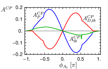
Fig. 13 shows the asymmetry in the production, APC​PA^{CP}_{P}, in the decay of H±→t​bH^{\pm}\to tb, AD,t​bC​PA^{CP}_{D,tb}, and the combined one, At​bC​P=APC​P+AD,t​bC​PA^{CP}_{tb}=A^{CP}_{P}+A^{CP}_{D,tb}, as a function of the phase ϕAt\phi_{A_{t}}. All three curves are symmetric for ϕAt→−ϕAt\phi_{A_{t}}\to-\phi_{A_{t}} because ϕμ=0\phi_{\mu}=0. APC​PA^{CP}_{P} and AD,t​bC​PA^{CP}_{D,tb} have negative relative signs with a maximium/minimum at |ϕAt|∼< 0.45​π|\phi_{A_{t}}|\;\raisebox{-3.87495pt}{$\textstyle\stackrel{{\scriptstyle\textstyle<}}{{\sim}}$}\;0.45\pi, with |APC​P|∼|A^{CP}_{P}|\sim 20% and |AD,t​bC​P|∼|A^{CP}_{D,tb}|\sim 16% there. Due to this cancellation the resulting asymmetry At​bC​PA^{CP}_{tb} is reduced to ∼< 4\;\raisebox{-3.87495pt}{$\textstyle\stackrel{{\scriptstyle\textstyle<}}{{\sim}}$}\;4%.

Refer to caption

Figure 13: The asymmetry AC​PA^{CP} at hadron level for the production and the decay into t​btb only, and the total one, for the chosen set of parameters (59) as a function of ϕAt\phi_{A_{t}}.

In order to avoid the cancellation, we can study the mass range of H±H^{\pm}, before the t~1​b~1\tilde{t}_{1}\tilde{b}_{1} channel opens. In this case, having in mind our results in [8], the CP effects in the decay will be negligible and CPV will arise mainly in the production process due to the vertex and box contributions with g~\tilde{g} in the loops. For instance, for mH+=m_{H^{+}}= 400 GeV and mg~=m_{\tilde{g}}= 450 GeV we get At​bC​P=−3A^{CP}_{tb}=-3%.

In Fig. 14 the total asymmetries At​bC​PA^{CP}_{tb} and Aν​τC​PA^{CP}_{\nu\tau} as functions of mg~m_{\tilde{g}} are shown for mH+=m_{H^{+}}= 550 GeV. Both asymmetries are negative. They have their largest values at mg~∼425m_{\tilde{g}}\sim 425 GeV, with Aν​τC​P∼−27A^{CP}_{\nu\tau}\sim-27 %, At​bC​P∼−12A^{CP}_{tb}\sim-12 %, and then they decrease to zero.

Refer to caption

Figure 14: The total asymmetry AC​PA^{CP} at hadron level for the chosen set of parameters (59) as a function of mg~m_{\tilde{g}}, mH+=550m_{H^{+}}=550 GeV. The (red) line denoted by t​btb corresponds to the case where H±H^{\pm} decays to t​btb, and the (green) one denoted by τ​ντ\tau\nu_{\tau} to H±H^{\pm} decay to τ​ντ\tau\nu_{\tau}.

In Fig. 15 the dependence of At​bC​PA^{CP}_{tb} on the absolute value of AtA_{t} is shown for three different values of mH+m_{H^{+}}.

Refer to caption

Figure 15: The total asymmetry At​bC​PA_{tb}^{CP} at hadron level for the chosen set of parameters (59) as a function of |At||A_{t}|, for three values of mH+m_{H^{+}} (in GeV).

Refer to caption

Figure 16: The total asymmetry AC​PA^{CP} at hadron level for the chosen set of parameters (59) as a function of tan⁡β\tan\beta, mg~=450m_{\tilde{g}}=450 GeV, mH+=550m_{H^{+}}=550 GeV. The (red) line denoted by t​btb corresponds to the case where H±H^{\pm} decays to t​btb, and the (green) one denoted by τ​ντ\tau\nu_{\tau} corresponds to H±H^{\pm} decay to τ​ντ\tau\nu_{\tau}.

As already mentioned in the introduction, the phase of μ\mu is strongly constrained by the measurements of the EDMs. Nevertheless, we also studied the dependence of AC​PA^{CP} on ϕμ\phi_{\mu}. Using μ=700​e−i​π3\mu=700\,e^{-i{\pi\over 3}} GeV instead of μ=−700\mu=-700 GeV, we get for mg~=450m_{\tilde{g}}=450 GeV in Fig. 14 the asymmetry At​bC​P∼−22A_{tb}^{CP}\sim-22%.

The tan⁡β\tan\beta dependence is shown on Fig. 16, for f=t​bf=tb and f=τ​ντf=\tau\nu_{\tau}. In both considered cases the asymmetry AC​PA^{CP} has its maximum at tan⁡β∼5\tan\beta\sim 5, with At​bC​P∼12%A_{tb}^{CP}\sim 12\% and Aν​τC​P∼21%A_{\nu\tau}^{CP}\sim 21\%. It approximately vanishes for tan⁡β∼> 15\tan\beta\;\raisebox{-3.87495pt}{$\textstyle\stackrel{{\scriptstyle\textstyle>}}{{\sim}}$}\;15.

We have compared our results with those in [13, 14]. Our numerical results are in good agreement with [13], but we disagree analytically and numerically with [14], where in addition the box contributions are missing.

The production rate of H+H^{+} at the LHC for mH+=m_{H^{+}}= 550 GeV and tan⁡β=5\tan\beta=5 is ∼15\sim 15 fb (including a K-factor from QCD of 1.5, see [22]), and the BR(H+→t​bH^{+}\to tb) ∼\sim 20%. For an integrated luminosity of 200 fb-1 we get N∼600N\sim 600 and N=25\sqrt{N}=25. For mg~=450m_{\tilde{g}}=450 we get At​bC​P∼0.12A^{CP}_{tb}\sim 0.12 and therefore the statistical significance N​At​bC​P∼4\sqrt{N}A^{CP}_{tb}\sim 4. But because of the large background, the actual signal production rate will be most likely reduced and the statistical significance might be too low for a clear observation in H±​tH^{\pm}t production in the first stage of LHC. However, at SLHC with a design luminosity bigger by a factor of ∼\sim 10, such a measurement would be worth of being performed.

6 Conclusions

The MSSM with complex parameters in particular with AtA_{t} complex, gives rise to CP violation in the production of H±H^{\pm}, p​p→H±​t+Xpp\to H^{\pm}t+X, and in the decays of H±H^{\pm} to t​b,ντ​τ±tb,\,\nu_{\tau}\tau^{\pm} and W±​h0W^{\pm}h^{0} at one-loop level. We have calculated the corresponding asymmetries between the H+H^{+} and H−H^{-} rates both in the production and in the decays. A few improvements have been made with respect to previous calculations.

We have performed a detailed numerical analysis studying the dependence on the important parameters. A peculiarity is that in the case of p​p→H±​t+Xpp\to H^{\pm}t+X with H±→t​bH^{\pm}\to tb, the contributions coming from the selfenergy graph with t~​b~\tilde{t}\tilde{b} in the loop in the production and in the decay exactly cancel. Nevertheless, the asymmetry can go up to ∼12\sim 12% for mH+≃550m_{H^{+}}\simeq 550 GeV, mainly due to the box graphs with gluino in the production process. A measurement of the CP violating asymmetries at LHC can give important information of the parameters of the MSSM, especially on AtA_{t} and its phase.

Acknowledgments

The authors acknowledge support from EU under the MRTN-CT-2006-035505 network programme. This work is supported by the ”Fonds zur Förderung der wissenschaftlichen Forschung” of Austria, project No. P18959-N16. The work of E. C. and E. G. is partially supported by the Bulgarian National Science Foundation, grant 288/2008.

Appendix A Masses and mixing matrices

The mass matrix of the stops in the basis (t~L,t~R)(\tilde{t}_{L},\,\tilde{t}_{R}) reads

ℳt~2=(MQ~2+mZ2​cos⁡2​β​(12−23​sin2⁡θW)+mt2(At∗−μ​cot⁡β)​mt(At−μ∗​cot⁡β)​mtMU~2+23​mZ2​cos⁡2​β​sin2⁡θW+mt2).\hskip-28.45274pt{\cal M}_{\tilde{t}}^{2}={\small\left(\begin{array}[]{cc}M_{\tilde{Q}}^{2}+m_{Z}^{2}\cos 2\beta(\frac{1}{2}-\frac{2}{3}\sin^{2}\theta_{W})+m_{t}^{2}&(A_{t}^{*}-\mu\cot\beta)\,m_{t}\\ (A_{t}-\mu^{*}\cot\beta)\,m_{t}&M_{\tilde{U}}^{2}+\frac{2}{3}m_{Z}^{2}\cos 2\beta\sin^{2}\theta_{W}+m_{t}^{2}\end{array}\right)}\,. (62)

ℳt~2{\cal M}_{\tilde{t}}^{2} is diagonalized by the rotation matrix ℛt~{\cal R}^{\,\tilde{t}} such that ℛt~†ℳt~2ℛt~=diag(mt~12,mt~22){\cal R}^{\,\tilde{t}\,\dagger}\,{\cal M}_{\tilde{t}}^{2}\,{\cal R}^{\,\tilde{t}}={\rm diag}(m_{\tilde{t}_{1}}^{2},\,m_{\tilde{t}_{2}}^{2}) and (t~Lt~R)=ℛt~​(t~1t~2){\scriptsize\Big(\!\!\begin{array}[]{cc}\tilde{t}_{L}\\ \tilde{t}_{R}\end{array}\!\!\Big)}={\cal R}^{\tilde{t}}\,{\scriptsize\Big(\!\!\begin{array}[]{cc}\tilde{t}_{1}\\ \tilde{t}_{2}\end{array}\!\!\Big)}.

We have

ℛt~=(ℛL​1t~ℛL​2t~ℛR​1t~ℛR​2t~)=(ei2​φt~cosθt~−ei2​φt~sinθt~e−i2​φt~sinθt~e−i2​φt~cosθt~).{\cal R}^{\,\tilde{t}}=\left(\begin{array}[]{rr}{\cal R}^{\,\tilde{t}}_{L1}&{\cal R}^{\,\tilde{t}}_{L2}\\ {\cal R}^{\,\tilde{t}}_{R1}&{\cal R}^{\,\tilde{t}}_{R2}\end{array}\right)=\left(\begin{array}[]{rr}e^{\frac{i}{2}\varphi_{\tilde{t}}}\cos\theta_{\tilde{t}}&-e^{\frac{i}{2}\varphi_{\tilde{t}}}\sin\theta_{\tilde{t}}\\ e^{-\frac{i}{2}\varphi_{\tilde{t}}}\sin\theta_{\tilde{t}}&e^{-\frac{i}{2}\varphi_{\tilde{t}}}\cos\theta_{\tilde{t}}\end{array}\right)\;. (63)

Analogously, the mass matrix of the sbottoms in the basis (b~L,b~R)(\tilde{b}_{L},\,\tilde{b}_{R})

ℳb~2=(MQ~2−mZ2​cos⁡2​β​(12−13​sin2⁡θW)+mb2(Ab∗−μ​tan⁡β)​mb(Ab−μ∗​tan⁡β)​mbMD~2−13​mZ2​cos⁡2​β​sin2⁡θW+mb2).\hskip-28.45274pt{\cal M}_{\tilde{b}}^{2}={\small\left(\begin{array}[]{cc}M_{\tilde{Q}}^{2}-m_{Z}^{2}\cos 2\beta(\frac{1}{2}-\frac{1}{3}\sin^{2}\theta_{W})+m_{b}^{2}&(A_{b}^{*}-\mu\tan\beta)\,m_{b}\\ (A_{b}-\mu^{*}\tan\beta)\,m_{b}&M_{\tilde{D}}^{2}-\frac{1}{3}m_{Z}^{2}\cos 2\beta\sin^{2}\theta_{W}+m_{b}^{2}\end{array}\right)}\,. (64)

is diagonalized by the rotation matrix ℛb~{\cal R}^{\,\tilde{b}} such that ℛb~†ℳb~2ℛb~=diag(mb~12,mb~22){\cal R}^{\,\tilde{b}\,\dagger}{\cal M}_{\tilde{b}}^{2}\,{\cal R}^{\,\tilde{b}}={\rm diag}(m_{\tilde{b}_{1}}^{2},\,m_{\tilde{b}_{2}}^{2}). ℛb~{\cal R}^{\,\tilde{b}} has the same structure like ℛt~{\cal R}^{\,\tilde{t}} given with (63), and one can obtain it by making the interchange t~→b~\tilde{t}\rightarrow\tilde{b}.

Appendix B Interaction Lagrangian

The part of the MSSM interaction Lagrangian used in our analytical calculations is given in this section.

The interaction of the charged Higgs boson with two quarks reads

ℒH±​t​b=H+​t¯​(yt​PL+yb​PR)​b+H−​b¯​(yb​PL+yt​PR)​t,{\cal L}_{H^{\pm}tb}=H^{+}\,\bar{t}\,(y_{t}P_{L}+y_{b}P_{R})\,b+H^{-}\,\bar{b}\,(y_{b}P_{L}+y_{t}P_{R})\,t\,, (65)

where the PLP_{L} and PRP_{R} are the left/ right projection operators

PL=12​(1−γ5),PR=12​(1+γ5),P_{L}=\frac{1}{2}(1-\gamma_{5})\,,\quad P_{R}=\frac{1}{2}(1+\gamma_{5})\,,

yty_{t} and yby_{b} are the tree-level couplings

yt=ht​cos⁡β,yb=hb​sin⁡β,y_{t}=h_{t}\cos\beta\,,\qquad y_{b}=h_{b}\sin\beta\,, (66)

with hth_{t} and hbh_{b} - the top and bottom Yukawa couplings

ht=g2​mW​1sin⁡β,hb=g2​mW​1cos⁡β.h_{t}=\frac{g}{\sqrt{2}m_{W}}\frac{1}{\sin\beta}\,,\qquad h_{b}=\frac{g}{\sqrt{2}m_{W}}\frac{1}{\cos\beta}\,. (67)

The interaction of two quarks with gluon exchange is given by

ℒq​q​g=−gs​Ti​ja​Gμa​q¯i​γμ​qj,{\cal L}_{qqg}\,=\,-g_{s}\,T^{a}_{\!ij}\,G^{a}_{\!\mu}\,\bar{q}_{i}\,\gamma^{\mu}\,q_{j}\,, (68)

with i,j=1,2,3i,j=1,2,3 and a=1,..,8a=1,..,8.

The interaction of the charged Higgs boson with two squarks is described by

ℒH±​t~i​b~j=(G4)i​j​H+​t~i∗​b~j+(G4∗)i​j​H−​b~j∗​t~i,{\cal L}_{H^{\pm}\tilde{t}_{i}\tilde{b}_{j}}=(G_{4})_{ij}\,H^{+}\,\tilde{t}_{i}^{*}\,\tilde{b}_{j}+(G_{4}^{*})_{ij}\,H^{-}\,\tilde{b}_{j}^{*}\,\tilde{t}_{i}\,, (69)

with i,j=1,2i,j=1,2,

G4=ℛt~†G^4ℛb~,G_{4}={\cal R}^{\,\tilde{t}\,\dagger}\;\hat{G}_{4}\;{\cal R}^{\,\tilde{b}}\,, (70)

and the matrix G^4\hat{G}_{4} is given by

G^4=(hb​mb​sin⁡β+ht​mt​cos⁡β−2​g​mW​sin⁡β​cos⁡βhb​(Ab∗​sin⁡β+μ​cos⁡β)ht​(At​cos⁡β+μ∗​sin⁡β)ht​mb​cos⁡β+hb​mt​sin⁡β).\hskip-28.45274pt\hat{G}_{4}={\small\left(\!\begin{array}[]{cc}h_{b}m_{b}\sin\beta+h_{t}m_{t}\cos\beta-\sqrt{2}\,g\,m_{W}\sin\beta\cos\beta&h_{b}\,(A_{b}^{*}\sin\beta+\mu\cos\beta)\\[8.53581pt] h_{t}\,(A_{t}\cos\beta+\mu^{*}\sin\beta)&h_{t}m_{b}\cos\beta+h_{b}m_{t}\sin\beta\end{array}\!\right)}\,. (71)

The W±W^{\pm}-squark-squark interaction Lagrangian reads

ℒW±​t~i​b~j=−i​g2(ℛL​it~ℛL​jb~∗Wμ−b~j∗∂μ↔μt~i+ℛL​it~∗ℛL​jb~Wμ+t~i∗∂μ↔μb~j),\displaystyle{\cal L}_{W^{\pm}\tilde{t}_{i}\tilde{b}_{j}}=-\frac{ig}{\sqrt{2}}\,({\cal R}_{Li}^{\tilde{t}}{\cal R}_{Lj}^{\tilde{b}*}\,W^{-}_{\mu}\,\tilde{b}_{j}^{*}\!\stackrel{{\scriptstyle\leftrightarrow}}{{\partial^{\mu}}}\!\tilde{t}_{i}+{\cal R}_{Li}^{\tilde{t}*}{\cal R}_{Lj}^{\tilde{b}}\,W^{+}_{\mu}\,\tilde{t}_{i}^{*}\!\stackrel{{\scriptstyle\leftrightarrow}}{{\partial^{\mu}}}\!\tilde{b}_{j})\,, (72)

where i,j=1,2i,j=1,2 and A∂μ↔μB=A⁡(∂μB)−(∂μA)​B.A\!\stackrel{{\scriptstyle\leftrightarrow}}{{\partial^{\mu}}}\!B=A\,(\partial_{\mu}B)-(\partial_{\mu}A)\,B.

The squark-quark-gluino interaction is given by

ℒq​q~​g~=−2gsTj​ka[g~¯a(ℛL​iq~∗e−i2​ϕ3PL−ℛR​iq~∗ei2​ϕ3PR)qkq~ij∗\displaystyle{\cal L}_{q\tilde{q}\tilde{g}}=-\sqrt{2}\,g_{s}\,T_{jk}^{a}\left[\,\bar{\tilde{g}}_{a}({\cal R}_{Li}^{\tilde{q}*}\,e^{-\frac{i}{2}\phi_{3}}P_{L}-{\cal R}_{Ri}^{\tilde{q}*}\,e^{\frac{i}{2}\phi_{3}}P_{R})\,q^{k}\,\tilde{q}_{i}^{j*}\right.
+q¯j(ℛL​iq~ei2​ϕ3PR−ℛR​iq~e−i2​ϕ3PL)g~aq~ik],\displaystyle\hskip 85.35826pt\left.+\,\bar{q}^{j}({\cal R}_{Li}^{\tilde{q}}\,e^{\frac{i}{2}\phi_{3}}P_{R}-{\cal R}_{Ri}^{\tilde{q}}\,e^{-\frac{i}{2}\phi_{3}}P_{L})\,\tilde{g}_{a}\,\tilde{q}_{i}^{k}\,\right]\,,\qquad (73)

with i=1,2i=1,2, j,k=1,2,3j,k=1,2,3, and a=1,..8a=1,..8.

The interaction of two quarks with W-boson exchange is described by

ℒW±​t​b=−g2​(Wμ+​t¯​γμ​PL​b+Wμ−​b¯​γμ​PL​t).{\cal L}_{W^{\pm}tb}\,=\,-\frac{g}{\sqrt{2}}\,(W^{+}_{\mu}\,\bar{t}\,\gamma^{\mu}\,P_{L}\,b+W^{-}_{\mu}\,\bar{b}\,\gamma^{\mu}\,P_{L}\,t)\,. (74)

Appendix C Passarino-Veltman integrals

The definitions of the Passarino–Veltman two-, and three-point functions [23] in the convention of [24] and the derived analytical expressions for their imaginary parts [10, 25] are given in this section.

The PV two-point functions are defined through the 4-dimensional integrals, as

B0​(p12,m02,m12)\displaystyle B_{0}(p_{1}^{2},m_{0}^{2},m_{1}^{2}) =\displaystyle= 1i​π2​∫dD​q​1𝒟0​𝒟1,\displaystyle\frac{1}{i\pi^{2}}\int d^{D}\!q\>\frac{1}{{\mathcal{D}}^{0}{\mathcal{D}}^{1}}\,, (75)
Bμ​(p12,m02,m12)\displaystyle B_{\mu}(p_{1}^{2},m_{0}^{2},m_{1}^{2}) =\displaystyle= 1i​π2​∫dD​q​qμ𝒟0​𝒟1=p1​μ​B1​(p12,m02,m12),\displaystyle\frac{1}{i\pi^{2}}\int d^{D}\!q\>\frac{q_{\mu}}{{\mathcal{D}}^{0}{\mathcal{D}}^{1}}=p_{1\mu}\,B_{1}(p_{1}^{2},m_{0}^{2},m_{1}^{2})\,, (76)

where we use the notation

𝒟0=q2−m02and𝒟j=(q+pj)2−mj2.{\mathcal{D}}^{0}=q^{2}-m_{0}^{2}\quad\mbox{and}\quad{\mathcal{D}}^{j}=(q+p_{j})^{2}-m_{j}^{2}\,. (77)

In the rest frame system of the (decaying) particle with impulse p1p_{1}, for the imaginary part of B0B_{0} we get

Im​B0​(M12,m02,m12)=π​λ1/2​(M12,m02,m12)M12,\displaystyle{\rm Im}\,B_{0}(M_{1}^{2},m_{0}^{2},m_{1}^{2})=\frac{\pi\lambda^{1/2}(M_{1}^{2},m_{0}^{2},m_{1}^{2})}{M_{1}^{2}}\,, (78)

where the λ\lambda-function is defined as

λ⁡(x,y,z)\displaystyle\lambda(x,y,z) =\displaystyle= x2+y2+z2−2​x​y−2​x​z−2​y​z.\displaystyle x^{2}+y^{2}+z^{2}-2xy-2xz-2yz. (79)

In order to derive the imaginary part of B1B_{1} we use the relation

2​k2​B1​(k2,m02,m12)=A0​(m02)−A0​(m12)+(m12−m02−k2)​B0​(k2,m02,m12).\displaystyle 2k^{2}B_{1}(k^{2},m_{0}^{2},m_{1}^{2})=A_{0}(m_{0}^{2})-A_{0}(m_{1}^{2})+(m_{1}^{2}-m_{0}^{2}-k^{2})B_{0}(k^{2},m_{0}^{2},m_{1}^{2})\,. (80)

Having in mind that Im​A0​(m2)=0{\rm Im}\,A_{0}(m^{2})=0, we obtain

Im​B1​(M12,m02,m12)=π⁡(m12−m02−M12)​λ1/2​(M12,m02,m12)2​M14.\displaystyle{\rm Im}\,B_{1}(M_{1}^{2},m_{0}^{2},m_{1}^{2})=\frac{\pi(m_{1}^{2}-m_{0}^{2}-M_{1}^{2})\lambda^{1/2}(M_{1}^{2},m_{0}^{2},m_{1}^{2})}{2M_{1}^{4}}\,. (81)

The PV three-point functions are defined as

C0​(p12,(p1−p2)2,p22,m02,m12,m22)\displaystyle C_{0}(p_{1}^{2},(p_{1}-p_{2})^{2},p_{2}^{2},m_{0}^{2},m_{1}^{2},m_{2}^{2}) =\displaystyle= 1i​π2​∫dD​q​1𝒟0​𝒟1​𝒟2,\displaystyle\frac{1}{i\pi^{2}}\int d^{D}\!q\>\frac{1}{{\mathcal{D}}^{0}{\mathcal{D}}^{1}{\mathcal{D}}^{2}}\,,
Cμ​(p12,(p1−p2)2,p22,m02,m12,m22)\displaystyle C_{\mu}(p_{1}^{2},(p_{1}-p_{2})^{2},p_{2}^{2},m_{0}^{2},m_{1}^{2},m_{2}^{2}) =\displaystyle= 1i​π2​∫dD​q​qμ𝒟0​𝒟1​𝒟2=p1​μ​C1+p2​μ​C2.\displaystyle\frac{1}{i\pi^{2}}\int d^{D}\!q\>\frac{q_{\mu}}{{\mathcal{D}}^{0}{\mathcal{D}}^{1}{\mathcal{D}}^{2}}=p_{1\mu}C_{1}+p_{2\mu}C_{2}\,.
Refer to caption
Figure 17: The selfenergy and vertex type diagrams corresponding to the PV two- and three-point integrals, when particles with masses m0m_{0} and m1m_{1} are on mass shell.

For the absorptive parts of the integrals C0,C1C_{0},C_{1} and C2C_{2} in () in the rest frame of the (decaying) particle with momentum p1p_{1}, when particles with masses m0m_{0} and m1m_{1} are on mass shell, Fig. 17, we obtain

Im​C0​(M12,M32,M22,𝐦𝟎𝟐,𝐦𝟏𝟐,m22)=−πλ1/2​(M12,M22,M32)​ln⁡|a+ba−b|\displaystyle{\rm Im}\,C_{0}(M_{1}^{2},M_{3}^{2},M_{2}^{2},{\bf m_{0}^{2},m_{1}^{2}},m_{2}^{2})=-\frac{\pi}{\lambda^{1/2}(M_{1}^{2},M_{2}^{2},M_{3}^{2})}\ln|\frac{a+b}{a-b}| (83)
Im​C1​(M12,M32,M22,𝐦𝟎𝟐,𝐦𝟏𝟐,m22)=M22​A−(p1​p2)​BΔ\displaystyle{\rm Im}\,C_{1}(M_{1}^{2},M_{3}^{2},M_{2}^{2},{\bf m_{0}^{2},m_{1}^{2}},m_{2}^{2})=\frac{M_{2}^{2}\,A-(p_{1}p_{2})\,B}{\Delta} (84)
Im​C2​(M12,M32,M22,𝐦𝟎𝟐,𝐦𝟏𝟐,m22)=−(p1​p2)​A−M12​BΔ\displaystyle{\rm Im}\,C_{2}(M_{1}^{2},M_{3}^{2},M_{2}^{2},{\bf m_{0}^{2},m_{1}^{2}},m_{2}^{2})=-\frac{(p_{1}p_{2})\,A-M_{1}^{2}\,B}{\Delta} (85)

Here we have

Δ=M12​M22−(p1​p2)2,(p1​p2)=M12+M22−M322,\displaystyle\Delta=M_{1}^{2}M_{2}^{2}-(p_{1}p_{2})^{2}\,,\qquad(p_{1}p_{2})=\frac{M_{1}^{2}+M_{2}^{2}-M_{3}^{2}}{2}\,,\qquad
a=M22+m02−m22+2​q0​p20,b=−2​|q→|​|p2→|,\displaystyle a=M_{2}^{2}+m_{0}^{2}-m_{2}^{2}+2\,q^{0}p_{2}^{0}\,,\qquad b=-2\,|\,\vec{q}\,|\,|\vec{p_{2}}\,|\,,\qquad\qquad
A=−π⁡(m12−m02−M12)2​λ1/2​(M12,M22,M32)​ln⁡|a+ba−b|,\displaystyle A=-\frac{\,\pi\,(m_{1}^{2}-m_{0}^{2}-M_{1}^{2})}{2\,\lambda^{1/2}(M_{1}^{2},M_{2}^{2},M_{3}^{2})}\,\ln|\frac{a+b}{a-b}|\,,\qquad\qquad
B=πλ1/2​(M12,M22,M32)​{12​(M22+m02−m22)​ln⁡|a+ba−b|+2​|q→|​|p2→|},\displaystyle B=\frac{\,\pi}{\lambda^{1/2}(M_{1}^{2},M_{2}^{2},M_{3}^{2})}\,\left\{\frac{1}{2}(M_{2}^{2}+m_{0}^{2}-m_{2}^{2})\ln|\frac{a+b}{a-b}|+2\,|\,\vec{q}\,|\,|\vec{p_{2}}\,|\right\},
q0​p20=(m12−m02−M12)​(M12+M22−M32)4​M12,\displaystyle q^{0}p_{2}^{0}=\frac{(m_{1}^{2}-m_{0}^{2}-M_{1}^{2})(M_{1}^{2}+M_{2}^{2}-M_{3}^{2})}{4M_{1}^{2}}\,,\qquad\qquad
|q→|​|p2→|=λ1/2​(M12,m02,m12)​λ1/2​(M12,M22,M32)4​M12.\displaystyle|\,\vec{q}\,|\,|\vec{p_{2}}\,|=\frac{\lambda^{1/2}(M_{1}^{2},m_{0}^{2},m_{1}^{2})\,\lambda^{1/2}(M_{1}^{2},M_{2}^{2},M_{3}^{2})}{4M_{1}^{2}}\,.\qquad\qquad (86)

In (83)-(85) and further, we denote masses of the on-shell particles with bold font. Generally, the functions C0,C1C_{0},C_{1} and C3C_{3} have three terms according to the three possible cuts over the particles in the loops, and which of them is non zero depends on the kinematics. The imaginary part of C0C_{0} reads

Im​C0​(M12,M32,M22,m02,m12,m22)=Im​C0​(M12,M32,M22,𝐦𝟎𝟐,𝐦𝟏𝟐,m22)+\displaystyle{\rm Im}\,C_{0}(M_{1}^{2},M_{3}^{2},M_{2}^{2},m_{0}^{2},m_{1}^{2},m_{2}^{2})={\rm Im}\,C_{0}(M_{1}^{2},M_{3}^{2},M_{2}^{2},{\bf m_{0}^{2},m_{1}^{2}},m_{2}^{2})+
+Im​C0​(M12,M32,M22,m02,𝐦𝟏𝟐,𝐦𝟐𝟐)+Im​C0​(M12,M32,M22,𝐦𝟎𝟐,m12,𝐦𝟐𝟐).\displaystyle+{\rm Im}\,C_{0}(M_{1}^{2},M_{3}^{2},M_{2}^{2},m_{0}^{2},{\bf m_{1}^{2},m_{2}^{2}})+{\rm Im}\,C_{0}(M_{1}^{2},M_{3}^{2},M_{2}^{2},{\bf m_{0}^{2}},m_{1}^{2},{\bf m_{2}^{2}})\,. (87)

In terms of the analytic formulas (83)-(85) we write

Im​C0​(M12,M32,M22,m02,m12,m22)=Im​C0​(M12,M32,M22,𝐦𝟎𝟐,𝐦𝟏𝟐,m22)+\displaystyle{\rm Im}\,C_{0}(M_{1}^{2},M_{3}^{2},M_{2}^{2},m_{0}^{2},m_{1}^{2},m_{2}^{2})={\rm Im}\,C_{0}(M_{1}^{2},M_{3}^{2},M_{2}^{2},{\bf m_{0}^{2},m_{1}^{2}},m_{2}^{2})+
+Im​C0​(M32,M12,M22,m22,𝐦𝟏𝟐,𝐦𝟎𝟐)+Im​C0​(M22,M32,M12,𝐦𝟎𝟐,m22,𝐦𝟏𝟐).\displaystyle+{\rm Im}\,C_{0}(M_{3}^{2},M_{1}^{2},M_{2}^{2},m_{2}^{2},{\bf m_{1}^{2},m_{0}^{2}})+{\rm Im}\,C_{0}(M_{2}^{2},M_{3}^{2},M_{1}^{2},{\bf m_{0}^{2}},m_{2}^{2},{\bf m_{1}^{2}})\,. (88)
Im​C1​(M12,M32,M22,m02,m12,m22)=Im​C1​(M12,M32,M22,𝐦𝟎𝟐,𝐦𝟏𝟐,m22)+\displaystyle{\rm Im}\,C_{1}(M_{1}^{2},M_{3}^{2},M_{2}^{2},m_{0}^{2},m_{1}^{2},m_{2}^{2})={\rm Im}\,C_{1}(M_{1}^{2},M_{3}^{2},M_{2}^{2},{\bf m_{0}^{2},m_{1}^{2}},m_{2}^{2})+
+Im​C1​(M32,M12,M22,m22,𝐦𝟏𝟐,𝐦𝟎𝟐)+Im​C2​(M22,M32,M12,𝐦𝟎𝟐,m22,𝐦𝟏𝟐),\displaystyle+{\rm Im}\,C_{1}(M_{3}^{2},M_{1}^{2},M_{2}^{2},m_{2}^{2},{\bf m_{1}^{2},m_{0}^{2}})+{\rm Im}\,C_{2}(M_{2}^{2},M_{3}^{2},M_{1}^{2},{\bf m_{0}^{2}},m_{2}^{2},{\bf m_{1}^{2}})\,, (89)
Im​C2​(M12,M32,M22,m02,m12,m22)=Im​C2​(M12,M32,M22,𝐦𝟎𝟐,𝐦𝟏𝟐,m22)+\displaystyle{\rm Im}\,C_{2}(M_{1}^{2},M_{3}^{2},M_{2}^{2},m_{0}^{2},m_{1}^{2},m_{2}^{2})={\rm Im}\,C_{2}(M_{1}^{2},M_{3}^{2},M_{2}^{2},{\bf m_{0}^{2},m_{1}^{2}},m_{2}^{2})+
+[ImC0(M32,M12,M22,m22,𝐦𝟏𝟐,𝐦𝟎𝟐)+ImC1(M32,M12,M22,m22,𝐦𝟏𝟐,𝐦𝟎𝟐)+\displaystyle+[{\rm Im}\,C_{0}(M_{3}^{2},M_{1}^{2},M_{2}^{2},m_{2}^{2},{\bf m_{1}^{2},m_{0}^{2}})+{\rm Im}\,C_{1}(M_{3}^{2},M_{1}^{2},M_{2}^{2},m_{2}^{2},{\bf m_{1}^{2},m_{0}^{2}})+
+ImC2(M32,M12,M22,m22,𝐦𝟏𝟐,𝐦𝟎𝟐)]+ImC1(M22,M32,M12,𝐦𝟎𝟐,m22,𝐦𝟏𝟐).\displaystyle+{\rm Im}\,C_{2}(M_{3}^{2},M_{1}^{2},M_{2}^{2},m_{2}^{2},{\bf m_{1}^{2},m_{0}^{2}})]+{\rm Im}\,C_{1}(M_{2}^{2},M_{3}^{2},M_{1}^{2},{\bf m_{0}^{2}},m_{2}^{2},{\bf m_{1}^{2}})\,.\, (90)

References

  • [1] M. Dugan, B. Grinstein and L. J. Hall, Nucl. Phys. B 255 (1985) 413.
  • [2] M. Carena, M. Quiros and C. E. Wagner, Nucl. Phys. B 524 (1998) 3 [hep-ph/9710401]; for a review see: A. G. Cohen, D. B. Kaplan and A. E. Nelson, Ann. Rev. Nucl. Part. Sci. 43 (1993) 27 [hep-ph/9302210].
  • [3] I. S. Altarev et al., Phys. Lett. B 276 (1992) 242; I. S. Altarev et al., Phys. Atom. Nucl. 59 (1996) 1152 [Yad. Fiz. 59N7 (1996) 1204]; E. D. Commins, S. B. Ross, D. DeMille and B. C. Regan, Phys. Rev. A 50 (1994) 2960.
  • [4] P. Nath, Phys. Rev. Lett. 66 (1991) 2565; Y. Kizukuri and N. Oshimo, Phys. Rev. D 46 (1992) 3025; R. Garisto and J. D. Wells, Phys. Rev. D 55 (1997) 1611 [hep-ph/9609511]; Y. Grossman, Y. Nir and R. Rattazzi, Adv. Ser. Direct. High Energy Phys. 15 (1998) 755 [hep-ph/9701231].
  • [5] A. Pilaftsis, Phys. Rev. D 58 (1998) 096010 [hep-ph/9805373] and Phys. Lett. B 435 (1998) 88 [hep-ph/9805373; A. Pilaftsis and C. E. Wagner, Nucl. Phys. B 553 (1999) 3 [hep-ph/9902371]; D. A. Demir, Phys. Rev. D 60 (1999) 055006 [hep-ph/9901389].
  • [6] M. Carena, J. R. Ellis, A. Pilaftsis and C. E. Wagner, Nucl. Phys. B 586 (2000) 92 [hep-ph/0003180].
  • [7] For a review, see D. Atwood, S. Bar-Shalom, G. Eilam and A. Soni, Phys. Rept. 347 (2001) 1 [hep-ph/0006032].
  • [8] E. Christova, H. Eberl, E. Ginina, W. Majerotto, JHEP 0702 (2007) 075 [hep-ph/0612088].
  • [9] E. Christova, H. Eberl, S. Kraml and W. Majerotto, JHEP 0212 (2002) 021 [hep-ph/0211063].
  • [10] E. Christova, E. Ginina, M. Stoilov JHEP 11 (2003) 027 [hep-ph/0307319].
  • [11] E. Ginina, contribution to the 4th workshop ”Gravity, Astrophysics, and Strings at the Black Sea”, 2007, hep-ph/0801.2344
  • [12] E. Christova, H. Eberl, E. Ginina, arXiv:0812.0265 [hep-ph].
  • [13] J. William, contributions to CPNSH Report, CERN-2006-009 (hep-ph/0608079)
  • [14] Kang Young Lee, Dong-Won Jung, H. S. Song, Phys. Rev. D 70 (2004) 117701 [hep-ph/0307246].
  • [15] N. Kidonakis, JHEP 0505 (2005) 011, [hep-ph/0412422].
  • [16] E. Christova, H. Eberl, S. Kraml and W. Majerotto, Nucl. Phys. B 639 (2002) 263; E. Christova, H. Eberl, S. Kraml and W. Majerotto, Erratum to Nucl. Phys. B 639 (2002) 263.
  • [17] T. Hahn, Nucl. Phys. Proc. Suppl. B 89 (2000) 231; T. Hahn, FeynArts User’s Guide, Comp. Phys. Commun. 140 (2001) 418; T. Hahn, M. Perez-Victoria, FormCalc User’s Guide, Comput. Phys. Commun. 118 (1999) 153; T. Hahn, M. Perez-Victoria, LoopTools User’s Guide, Comput. Phys. Commun. 118 (1999) 153. (The software and all manuals are available at http://www.feynarts.de.)
  • [18] G. J. van Oldenborgh, Comput. Phys. Commun. 66 (1991) 1.
  • [19] J. Pumplin, D.R. Stump, J. Huston, H.L. Lai, Pavel M. Nadolsky, W.K. Tung, JHEP 12 (2002) 0207 [hep-ph/0201195].
  • [20] M. Battaglia et al., Eur. Phys. J. C 22 (2001) 535, [arXiv:hep-ph/0106204].
  • [21] A. Bartl, K. Hidaka, Y. Kizukuri, T. Kon, W. Majerotto, Phys. Lett. B 315 (1993) 360.
  • [22] A. Belyaev, D. Garcia, J. Guasch and J. Sola, hep-ph/0203031.
  • [23] G. Passarino and M. J. Veltman, Nucl. Phys. B 160 (1979) 151.
  • [24] A. Denner, Fortschr. Phys. 41 (1993) 307.
  • [25] M. Frank, I. Turan, Phys. Rev. D 76 (2007) 016001, [hep-ph/0703184].