One-loop electroweak effects on
stop-chargino production at LHC
Abstract
The process of stop-chargino production at LHC has been calculated in the Minimal Supersymmetric Standard Model at the complete electroweak one-loop level, assuming a mSUGRA symmetry breaking scheme. Several properties of the angular and invariant mass distributions of the basic amplitudes have been derived. For a meaningful collection of different benchmark points the overall electroweak one-loop effects are at most of the order of a few percent. At the realistically expected LHC accuracy, the main supersymmetric electroweak features of the process can be therefore essentially derived in this theoretical scheme from the simple Born level expressions.
I Introduction
The process of associated stop-chargino production at LHC has been
recently considered as a potential source of information on SUSY
parameters. In particular, it has been shown that the total rate would
exhibit a possibly relevant dependence on [1]
and could also be sensitive to possible deviations from a
Minimal Flavor Violation scheme [2]. In both cases, the
calculations have been performed at the lowest electroweak order. SUSY
QCD effects have been computed at NLO [3]. The conclusion
was that these NLO strong supersymmetric effects in general enhance the
LO total cross sections significantly, and thus must be carefully taken into
account.
If Supersymmetry were discovered at LHC, and measurements of stop-chargino
production began to be performed, the reasonable question would
arise of whether the NLO electroweak supersymmetric effects might
effectively change the special and relevant SUSY parameter dependence
of the lowest order expressions given in Refs. [1, 2],
in which case they should be also carefully taken into account, like the NLO QCD component.
The aim of this paper is precisely that of performing an accurate calculation of
the complete one-loop electroweak supersymmetric contributions to the
stop-chargino production process. As a preliminary approach, we shall
work in the Minimal Supersymmetric Standard Model, accept the validity
of a mSUGRA symmetry breaking scheme and select a number of
meaningful “benchmark” points to produce the final numerical
predictions.
Technically speaking, the paper is organized as follows. Sect.II will be
devoted to a description of the shape and of the basic properties of the
parton level amplitudes for at Born and at one-loop
level.
A detailed analysis at Born level of the dependence of the total rate
on supersymmetric parameters will be performed.
Illustrations will be given for the angular distributions and for the
invariant mass dependence of the helicity amplitudes near threshold and in
the high energy range, where we have checked the agreement with the
logarithmic terms of the Sudakov expansion. Sect.III will exhibit the
numerical one-loop effects on the production rates for a selected number
of typical SUSY benchmark points. As a general feature, the effects will
turn out to be numerically small, of a relative few percent at most, which
would hardly be effective at the realistically expected LHC experimental
accuracy.
II Kinematics and Amplitudes of the process
The kinematics of the process is expressed in terms of the Dirac spinors and with the momenta:
| (1) |
| (2) |
and the gluon polarization vector:
| (3) |
referring to the helicity labels ,
, .
The angle refers to and .
We will use ,
and .
The top squark states are mixed states of
with an angle and the chargino
states are mixed states of gauginos
and Higgsinos with matrix elements .
The process will be described by 8 helicity amplitudes
related to the
8 invariant amplitudes ( and ):
| (4) |
| (5) |
| (6) |
with . A colour matrix element
relating the initial
quark and the final squark has been
systematically factorized out.
Averaging over initial spins and colours and summing over final spins and colours
with:
| (7) |
leads to the elementary cross section:
| (8) |
where , .
The 8 scalar functions are obtained
in terms of Born and one-loop diagrams.
The Born terms result from the s-channel b exchange
and the u-channel exchange:
| (9) |
| (10) |
with the couplings:
| (11) |
Using the Dirac decomposition explicitly given in App. A of [1] one gets
the Born contribution to the 8 helicity amplitudes. Let us notice their
basic properties which will be essential to understand the final results.
First, because of the small value of , the helicity corresponds
to the chirality (L for and R for ).
In the case of the production of the lightest chargino () this means that
the amplitudes will generally dominate because the R
chirality couplings (see eq.(11)) are depressed by the factor
and by the non-diagonal chargino mixing element .
One can then predict the main features of the angular and of the energy
dependences using again App. A of [1]. At low energy (near above threshold)
the u-channel contribution is suppressed by the final momentum .
Only the s-channel contribution survives and the leading amplitudes
should be and . They respectively produce an angular
distribution and . Having the same magnitude
(at Born level) the unpolarized cross section should then be flat.
At high energy one observes a cancellation between the
s-channel and the u-channel Born contributions to , ,
, (see App.A of [1]), as well as the mass suppression
of the u-channel contribution to , (because
and tend to ). The only surviving amplitudes at high
energy are then and :
| (12) |
In this high energy limit the quantities of Eq.(12) can be expressed in terms of 3 basic amplitudes, one of gaugino type and two of higgsino type , . In all cases the high energy distribution should tend to a shape. For production and for the reasons already given above, should dominate. For a light stop , mixture of and , this amplitude will be:
| (13) |
II.1 Parameter Dependence at Born Level
Remaining at Born level it is already possible to extract
relevant e.w. information from the process.
Although some preliminary search of this kind already exists [1, 2],
we will devote this Section to a brief updated summary of the main information that could
be derived from this approximate treatment.
Indeed, at Born level a limited set of parameters affects the determination of physical observables.
Besides the values of the stop and chargino masses, which are obviously crucial for
the definition of the production threshold, other SUSY parameters contribute
to the the coupling , Eq.(11).
While explicitly appears in the various terms, the chargino
mixing matrices depend in a non-trivial way on parameters of
the chargino mass matrix:
Moreover, for production of physical stops, the mixing angle mixes the various terms of Eq.(11). In conclusion, it is possible to identify a set of independent parameters which determine the amplitude at Born level:
| (17) |
The chargino masses are determined by a combination of ,
and . Since to perform a parameter analysis of the process it
seems reasonable to fix all the masses, it is possible to trade, e.g.,
for and for , depending on the chargino of
the final state.
Given these premises, the process of production of the lightest stop and
chargino will now be analyzed at Born level to
investigate possible dependences on supersymmetric parameters. Rather than
looking for a dependence of the cross section on the stop or chargino masses
that we assumed to be experimentally known from previous discovery, we looked
for dependences on , and . The results of
the analysis are shown in Fig. 1: All panels show the
dependence of the total cross section on the mixing angle
for different values of , at different values of . In
particular, Figs. 1 and 1 show the
results obtained for low values of , close to the chargino mass, while in
Figs. 1 and 1 has been pushed to
the value of 800Gev, which is high compared to . It is possible to
notice that the cross section depends very strongly on the value of
and that there is always a value of the angle for which
the cross section drops near to zero. In Fig. 1, where
the low threshold allows a cross section of the order of the pb, it is
possible to see that changes from 6 pb for to less than 0.5 pb for
(when ). Therefore there are regions of the parameter space
where, even if the masses of final state particles are very low, the stop
mixing angle pushes the cross section to nearly undetectable levels.
The dependence on can indeed be understood looking
at the amplitude, which is a sum of terms of the form:
| (18) |
Depending on the values of and , the squared amplitude
generates the curves shown in Fig. 1.
The results also depend in a weaker and less trivial way on .
The cross section is pushed to somewhat higher values as
increases, but to different extents in the various considered cases:
the variation of the total cross sections with different values of
are strongly affected by the choice of resulting in a very mild
dependence on for high values of and viceversa,
so that the determination of this supersymmetric parameter from this process
could be ambiguous, unless the rate turns out to be larger than a certain
“threshold” value. Further constraints coming from other processes could
however limit the range of , and the determination of the two
remaining parameters through the analysis of this process would then be relevant.
II.2 One-Loop Amplitude
For the calculation of the one-loop amplitude we use the on-shell scheme; the one-loop electroweak terms can be classified in:
- —
counter terms for lines, coupling constants and mixing elements, all of them being expressed in terms of self-energy diagrams;
- —
self-energy corrections for and propagators;
- —
s-channel left and right triangles;
- —
u-channels bubbles with 4-leg couplings and up, down triangles;
- —
direct boxes, crossed boxes, twisted boxes;
Since the complete expressions of the various conter-terms and self
energies are rather involved we list them separately in the App. A.
All the contributions of the counter-terms and self energies, together with
the virtual vertex and box diagrams have been computed using the
usual decomposition in terms of Passarino-Veltman functions and
the complete amplitude has been implemented in the numerical code TigreMC.
We have checked the cancellation of the UV divergences
among counter terms, self-energies and triangles,
this cancellation occuring
separately for s-channel and for u-channel,
as well as for gauge-left, gauge-right, Yukawa-left and
Yukawa-right sectors separately.
Another useful check can be done using the high energy behaviour of the amplitudes.
High energy rules [4] predict the logarithmic
behaviour of these amplitudes at one-loop level.
They use splitting functions for external particles
, ,
and Renormalization Group effects on the parameters
appearing in the Born terms. They read:
| (19) | |||||
| (20) | |||||
| (21) | |||||
The logarithmic part of the gaugino amplitude (19) is similar to the
one obtained for the process with transverse [5].
Higgsino amplitudes ,
in (20,21) get logarithmic terms similar to the ones in both
for longitudinal and [6]. One notices that there is no linear
logarithmic contribution , but only quadratic logarithmic terms, in these Higgs or
Higgsino type of amplitudes. The coefficients of these quadratic logarithms
are of pure gauge origin and do not involve any free parameter.
Taking our complete one-loop computation and retaining only the logarithmic
parts of the B,C,D Passarino-Veltman functions appearing in the various diagrams, we do
recover the above expressions for the 3 types of leading amplitudes.
We now give illustrations of the various features mentioned above
for the process with production of the
lightest stop and chargino. We choose two typical benchmark MSSM points
called LS1 and LS2 whose characteristics are shown in Tab.1
together with those of all the benchmark points that we have used for the analysis (see next Section for more details).
| mSUGRA scenario | |||||||
|---|---|---|---|---|---|---|---|
| LS1 | 300 | 150 | -500 | 10 | + | 214.6 | 103.6 |
| LS2 | 300 | 150 | -500 | 50 | + | 224.7 | 106.9 |
| SPS5 | 150 | 300 | -1000 | 5 | + | 279.0 | 226.2 |
| SU1 | 70 | 350 | 0 | 10 | + | 566.4 | 255.7 |
| SU6 | 320 | 375 | 0 | 50 | + | 634.1 | 279.7 |
Fig. 6 shows the energy dependence of each helicity amplitude from threshold to high energy for a given (central) angle . For each amplitude two curves represent the Born and the full one loop result. One can check that they confirm the expectations described in the previous subsection, namely the nature of:
- —
the dominant amplitudes at low energy
- —
the dominant amplitudes at high energy
The size of the one-loop correction is of the order of few percent, and one
sees that the high energy behaviour is quickly reached as soon as the
threshold is crossed.
The difference between the LS1 and LS2 cases is due to the increase
in the final masses and in the change in the stop and in the chargino
mixings. In particular for LS2 the R chirality amplitudes are less
depressed because of the the difference in and in the mixing
element , which increase the value of (see Eq.(11)) and this can be clearly seen both
at low and at high energies.
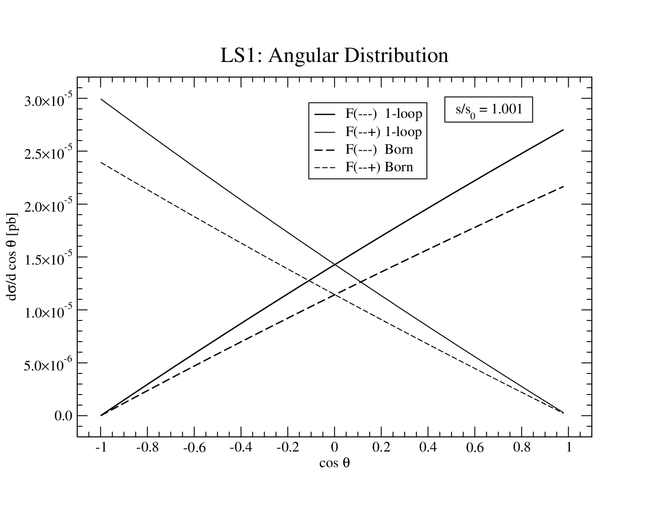
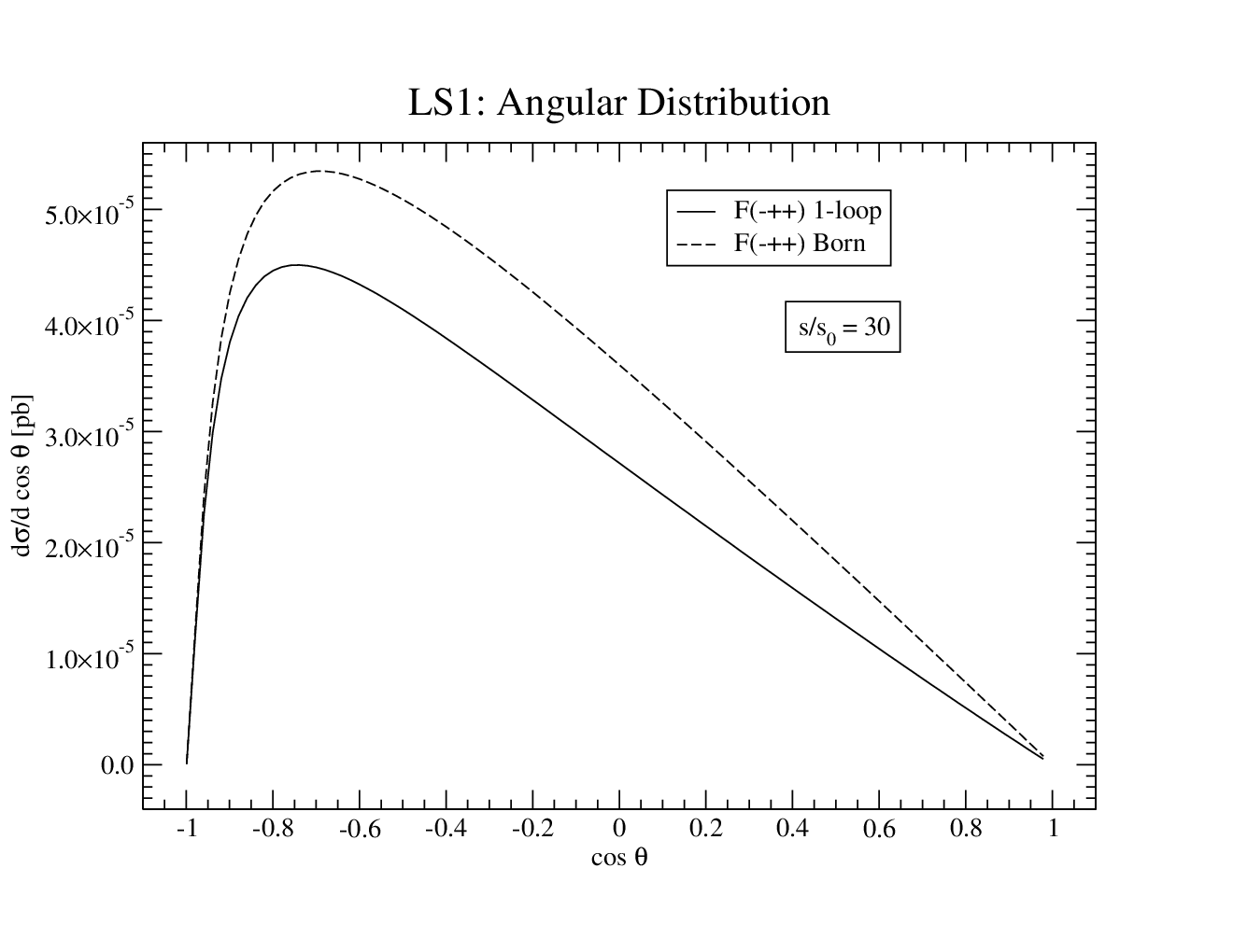
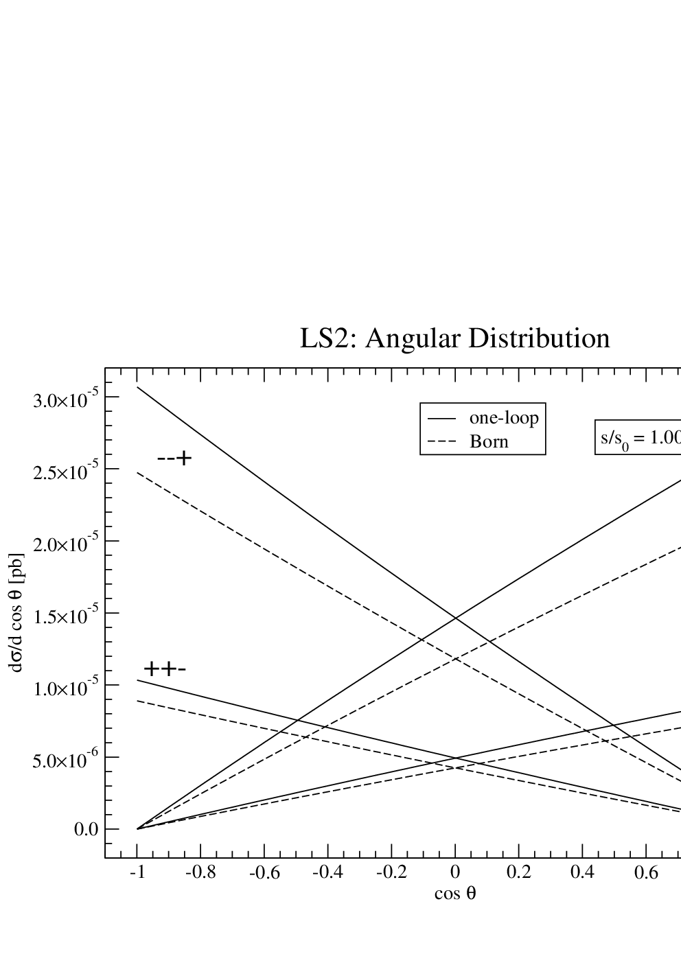
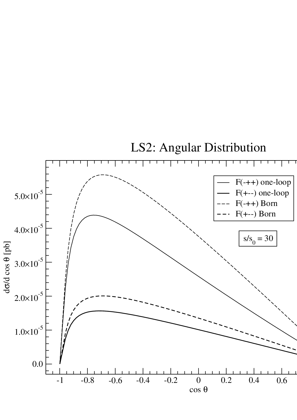
Fig. 7 gives the angular distributions at low energy () and at high
energy (). At low energy the leading amplitudes give indeed the
expected and distributions,
whereas at high energy one tends to a limiting
distribution, at least away from purely backward scattering.
The one-loop corrections make only little changes
in the shape of the angular distributions as expected from the
Sudakov rules.
II.3 QED radiation
The electroweak corrections include contributions
from virtual and from real photon emission. The virtual photon exchange
diagrams belong to the complete set of electroweak virtual corrections,
and are necessary for the gauge invariance of the final result.
The singularities associated with the massless nature of the photon have
been regularized by introducing a small photon mass .
The real radiation contribution has been split into a soft part,
derived within the eikonal approximation, where the photon energy has
been integrated from the lower bound to a maximum cut-off
, and into a hard part, integrated from
the minimum photon energy to the maximum
allowed kinematical value.
The soft real contribution
contains explicitly the photon mass parameter while the
hard part can be calculated with a massless external photon. The
complete
matrix element for real radiation, including fermion
mass effects,
has been calculated analytically with the help
of FeynArts [7]
and FormCalc [8].
The logarithmic terms containing cancel exactly in the sum of virtual and soft real part, leaving only polynomial spurious terms, which approach zero at least as . We have numerically checked the cancellation by taking the limit of our computation. The large collinear logarithms containing the bottom mass are only partially cancelled when real and virtual corrections are summed together, but they can be absorbed into the definition of the parton distribution functions (PDFs). This can be achieved redefining the bottom PDF according to a factorization scheme. In the (DIS) scheme such redefinition reads [9]
| (22) | |||||
with (). is the factorization scale, , while is the bottom charge. and are defined as follows,
| (23) |
The calculation of the full corrections to any hadronic observable must include QED effects in the DGLAP evolution equations. Such effects are taken into account in the MRST2004QED PDF [10]. This set is however NLO QCD, while our computation is leading order QCD. Therefore, analogously to [11], a LO QCD PDF set has been chosen, namely the CTEQ6L [12]. This choice is justified by the fact that QED effects are known to be small [13]. In the numerical analyses we have used the factorization scheme at the scale . It is worth to mention that the dependence of the full contribution on the factorization scheme is rather weak. Indeed, if the DIS factorization scheme is used instead of , the differences in the numerical value of the one-loop electroweak effects are of the order of 0.01% in all the considered mSUGRA benchmark points.
The final cross section has to be independent of the fictitious separator , for sufficiently small values. This has been checked numerically to hold for GeV, as shown in Figure 8 (lower panel), despite the strong sensitivity to of the soft plus virtual and of the hard cross section separately, as shown in Figure 8 (upper panel).
III One-Loop Results
The distribution of the invariant mass of the final states
has been evaluated at the one-loop electroweak level for a number of SUSY
benchmark points (assuming a mSUGRA supersymmetry breaking) with a wide
variation of mass spectra. The obtained cross sections
at the Born and one-loop level for five representative points (the ”Light SUSY”
LS1, LS2, discussed in [16], the ATLAS SU1 and SU6 [17] and the
SPS5 ”Light Stop scenario” [18]) are collected in Tab. 2: for
the realistic case of production of the lightest stop and chargino states
and ,
only the couple LS1 - LS2
give a cross section of order of the
(considering a global factor , arising from the conjugate process),
that we shall consider in this paper as a reasonable limit for realistic detections at the LHC.
All the other input sets, including the SPS5 ”Light Stop”, give smaller
rates, and will not be further considered in what follows.
For what concerns the one-loop electroweak corrections, we have found that they are generally small, of the order of a relative few percent for all the considered scenarios.
| mSUGRA scenario | Effect | ||
|---|---|---|---|
| LS1 | 0.4287 | 0.4442 | 3.6 |
| LS2 | 0.5419 | 0.5436 | 0.3 |
| SPS5 | 0.05704 | 0.05810 | 1.8 |
| SU1 | 0.004052 | 0.004041 | -0.3 |
| SU6 | 0.002541 | 0.002576 | 1.4 |
As an example of this behaviour in Figs. 9 and 10
we plot the differential distibutions for the LS1 and LS2 benchmark points,
(the points with highest cross sections): as one can notice, the
one-loop effect is positive in the low energy region
(near the production threshold) and drops to negative values increasing the final
invariant mass. The global effect on the totally integrated cross section,
being the result of the sum of two opposite contributions, is positive () in the LS1 case, slightly smaller and below the in the LS2 case.
The conclusion of our analysis is thus, for what concerns the possibility
that NLO electroweak effects might affect the stop-chargino production
process, essentially negative in the chosen theoretical scheme, given the
fact that a realistic experimental accuracy of the measurements of the
various rates should hardly be better than, say, ten percent or more
([19]). In this spirit, it appears that the
complete dependence on the SUSY parameters can be satisfactorily
provided by the simple Born expressions of the process discussed in the previous Section.
This conclusion is valid in the chosen theoretical scheme,
and is based on the relative smallness of the one-loop electroweak effects.
Clearly, the same conclusions cannot be drawn at this point for possible
different supersymmetric schemes. As a personal feeling, it seems unlikely
to us that strong one-loop effects might there arise, simply given the
unavoidably large sizes of the virtually exchanged sparticles. However, if
LHC discovered supersymmetry and reached a suitable experimental
accuracy, an extended analysis of the process that we have considered
might become definitely requested.
IV Conclusions
In this paper we have calculated the complete electroweak one-loop expression
of the stop-chargino process in the MSSM assuming a mSUGRA symmetry breaking
scheme, to evidentiate possible realistically “visible” effects.
In our calculations we have verified the
fulfillment of a number of theoretical requests, including the reproduction
of asymptotic Sudakov expansions. This, we believe, should make our analysis
reliable. As a result of our calculation we have concluded that the complete
one-loop electroweak effect is of the relative few percent size, that would
make it hardly visible in a realistic LHC situation.
Given this result, the relevant e.w. information can be extracted from the Born expression of the rate.
We have examined its possible dependence on those supersymmetric
parameters, on which it depends, that cannot be directly measured from direct
production, i.e. on the parameters , and . Assuming a
previous measurement of the stop and chargino masses, we have verified that
the dependence of the rates on and might be rather strong in the
case of light final state masses, and would influence the dependence on
. This would indicate that, given a light stop and chargino masses
picture, a measurement of the light stop-chargino process might provide an
original and useful type of constraints on the size of the relevant MSSM parameters.
Appendix A Counter Terms
The contributions to the s-channel of the counter terms terms are, symbolically:
| (24) | |||||
| (25) | |||||
| (26) | |||||
| (27) | |||||
and from s.e. one gets ( means ):
| (28) | |||||
| (29) | |||||
For the u-channel c.t. we obtain:
| (30) | |||||
| (31) | |||||
and from s.e.:
| (32) |
The renormalized self-energy is defined below. Following [20, 21, 22, 23] we have:
| (33) |
These results allow to write the renormalized stop self-energies as:
| (34) |
and for
| (35) |
The renormalization condition on the mixing angle is defined [22] in order to ensure the finiteness of the squark vertices.
| (36) |
which gives the needed:
| (37) |
The various cunter terms for the quarks and gauge bosons have the following explicit form in terms of self-energies; for b, t quark and gauge part:
| (38) |
| (39) |
| (40) |
| (41) |
| (42) |
| (43) |
while the couterterms for the gauge coupling lead to:
| (44) |
| (45) |
| (46) |
| (47) |
| (48) |
| (49) |
From [24] we have for :
| (50) |
| (51) |
We need also the counterterms for the chargino mixing matrices. Applying the method of [22] [24] requiring the cancellation of the antihermitean part of the wave function renormalization, we have:
| (52) |
| (53) |
| (54) |
Using the chargino c.t. and s.e. listed below the counter terms for are obtained from the field transformation:
| (55) |
They are obtained by applying the method proposed in [24] [25] [26] and in terms of the bubble of momentum they read:
| (56) |
with and:
| (57) |
| (58) |
and for
| (59) |
| (60) |
All the self-energy functions are computed from the diagrams of Fig. 3.
References
- [1] M. Beccaria, G. Macorini, L. Panizzi, F. M. Renard and C. Verzegnassi, Phys. Rev. D 74 (2006) 093009 [arXiv:hep-ph/0610075].
- [2] G. Bozzi, B. Fuks, B. Herrmann and M. Klasen, Nucl. Phys. B 787 (2007) 1 arXiv:0704.1826 [hep-ph].
- [3]
L. G. Jin, C. S. Li and J. J. Liu,
Eur. Phys. J. C 30 (2003) 77
[arXiv:hep-ph/0210362].
L. G. Jin, C. S. Li and J. J. Liu, Phys. Lett. B 561 (2003) 135 [arXiv:hep-ph/0307390]. - [4] M. Beccaria, F. M. Renard and C. Verzegnassi, [arXiv:hep-ph/0203254].
- [5] M. Beccaria, G. Macorini, F. M. Renard and C. Verzegnassi, Phys. Rev. D 73 (2006) 093001 [arXiv:hep-ph/0601175].
- [6] M. Beccaria, F. M. Renard and C. Verzegnassi, Phys. Rev. D 71 (2005) 033005 [arXiv:hep-ph/0410089].
- [7]
J. Kublbeck, M. Bohm and A. Denner,
Comput. Phys. Commun. 60, 165 (1990).
T. Hahn, Comput. Phys. Commun. 140, 418 (2001) [arXiv:hep-ph/0012260].
T. Hahn and C. Schappacher, Comput. Phys. Commun. 143, 54 (2002) [arXiv:hep-ph/0105349]. - [8]
T. Hahn and M. Perez-Victoria,
Comput. Phys. Commun. 118, 153 (1999)
[arXiv:hep-ph/9807565].
T. Hahn and M. Rauch, Nucl. Phys. Proc. Suppl. 157, 236 (2006) [arXiv:hep-ph/0601248]. - [9] U. Baur, S. Keller and D. Wackeroth, Phys. Rev. D 59, 013002 (1999) [arXiv:hep-ph/9807417].
- [10] A. D. Martin, R. G. Roberts, W. J. Stirling and R. S. Thorne, Eur. Phys. J. C 39, 155 (2005) [arXiv:hep-ph/0411040].
- [11] J. H. Kuhn, A. Kulesza, S. Pozzorini and M. Schulze, Nucl. Phys. B 797, 27 (2008) [arXiv:0708.0476 [hep-ph]].
- [12] J. Pumplin, D. R. Stump, J. Huston, H. L. Lai, P. M. Nadolsky and W. K. Tung, JHEP 0207, 012 (2002) [arXiv:hep-ph/0201195].
- [13] M. Roth and S. Weinzierl, Phys. Lett. B 590, 190 (2004) [arXiv:hep-ph/0403200].
- [14] M. Beccaria, C. M. Carloni Calame, G. Macorini, G. Montagna, F. Piccinini, F. M. Renard and C. Verzegnassi, Eur. Phys. J. C 53 (2008) 257 [arXiv:0705.3101 [hep-ph]].
- [15] M. Beccaria, C. M. Carloni Calame, G. Macorini, E. Mirabella, F. Piccinini, F. M. Renard and C. Verzegnassi, Phys. Rev. D 77 (2008) 113018 [arXiv:0802.1994 [hep-ph]].
- [16] M. Beccaria, G. Macorini, F. M. Renard and C. Verzegnassi, Phys. Rev. D 74, 013008 (2006) [arXiv:hep-ph/0605108].
- [17]
ATLAS Data Challenge 2 DC2 points:
http://paige.home.cern.ch/paige/fullsusy/romeindex.html. - [18] B. C. Allanach et al., The Snowmass points and slopes: Benchmarks for SUSY searches, in Proc. of the APS/DPF/DPB Summer Study on the Future of Particle Physics (Snowmass 2001) ed. N. Graf, In the Proceedings of APS / DPF / DPB Summer Study on the Future of Particle Physics (Snowmass 2001), Snowmass, Colorado, 30 Jun - 21 Jul 2001, pp P125 [arXiv:hep-ph/0202233].
- [19] B. Clément, ATL-SLIDE-2008-117; CERN-ATL-SLIDE-2008-117.
- [20] A. Djouadi, W. Hollik and C. Junger, Phys. Rev. D 55 (1997) 6975 [arXiv:hep-ph/9609419].
- [21] S. Kraml, H. Eberl, A. Bartl, W. Majerotto and W. Porod, Phys. Lett. B 386 (1996) 175 [arXiv:hep-ph/9605412].
- [22] H. Eberl, A. Bartl and W. Majerotto, Nucl. Phys. B 472 (1996) 481 [arXiv:hep-ph/9603206].
- [23] A. Arhrib and W. Hollik, JHEP 0404 (2004) 073 [arXiv:hep-ph/0311149].
- [24] L. H. Wan, W. G. Ma, R. Y. Zhang and Y. Jiang, Phys. Rev. D 64 (2001) 115004 [arXiv:hep-ph/0107089].
- [25] A. Denner and T. Sack, Nucl. Phys. B 347 (1990) 203.
- [26] B. A. Kniehl and A. Pilaftsis, Nucl. Phys. B 474, 286 (1996) [arXiv:hep-ph/9601390].