Bond Algebras and Exact Solvability of Hamiltonians:
Spin =1/2 Multilayer Systems and Other Curiosities
Abstract
We introduce an algebraic methodology for designing exactly-solvable Lie model Hamiltonians. The idea consists in looking at the algebra generated by bond operators. We illustrate how this method can be applied to solve numerous problems of current interest in the context of topological quantum order. These include Kitaev’s toric code and honeycomb models, a vector exchange model, and a Clifford model on a triangular lattice.
pacs
05.30.-d, 03.67.Pp, 05.30.Pr, 11.15.-qI Introduction
Whenever one is interested in studying a new physical phenomena whose effective model includes degrees of freedom (spins, fermions, bosons, etc.) which are strongly coupled, one attempts to invoke simplifying assumptions hoping that the resulting problem represents the relevant minimal model for the phenomenon at hand. Finding exactly-solvable models is always welcome. This paper is about a general methodology to generate exactly-solvable Hamiltonians by concentrating on the algebra generated by algebraic objects called bonds. We have already used this methodology in Ref. [1], where we solved a doped orbital compass model in two and three space dimensions, although we did not explained the generality of the mathematical approach. A goal of this paper is to present this methodology in full detail and show that by using the algebra of bond operators one can easily construct whole families of exactly-solvable models, several of these displaying topological quantum order [2], and spin liquid behavior.
For the sake of clarity, we will focus on quantum lattice systems which have sites, with the number of sites along each spatial direction , and the dimensionality of the lattice. The connectivity of the lattice and its general topology are of paramount importance. Associated with each lattice site there is a Hilbert space of finite dimension . The total Hilbert space is the tensor product of the local state spaces, , in the case of distinguishable subsystems (or a proper subspace in the case of indistinguishable ones), and its dimension is .
Let us first start with an intuitive introduction to the key concept of bond algebras. We consider situations in which the Hamiltonian of a system , whose state space is , can be written as a sum of quasi-local terms or bonds (),
| (1) |
where is a -number ( must be an Hermitian operator) and includes a finite number of lattice sites . In general, the operators will generate a certain (bond) algebra whose dimension is . To simplify the description, in the following, we are going to concentrate on semisimple Lie algebras. Notice that we do not constrain ourselves to a particular representation of the algebra.
It may happen that the Hamiltonian itself is an element of a subalgebra of of dimension poly. If such is the case, , which represents a Generalized Mean-Field Hamiltonian (GMFH), is exactly-solvable [3], and there is a polynomially in efficient algorithm to diagonalize it [3]. We say that is exactly-solvable when an arbitrarily chosen eigenvalue, and an appropriate description of the corresponding eigenstate, can be obtained and represented to precision by means of a classical algorithm efficient in and . This definition, motivated by complexity theory, yields a sufficient criterion for exact-solvability. A particular case of exact solvability is when the spectrum can be expressed in closed form.
A main contribution of this paper is to propose a methodology to generate such Hamiltonians by using two mathematical principles that will become evident in the following sections. In all cases, this methodology rests on (1) Topological constraints that are related to the connectivity of the lattice Hamiltonian or graph. In several instances, it further relies on the existence of (2) gauge symmetries. These symmetries allow a decomposition of the Hilbert space into sectors. The operators belong to the lowest dimensional representation of the algebra on the Hilbert space, or its sub-spaces. In the following we illustrate the bond algebra methodology by showing some tutorial examples of known trivially exactly-solvable problems.
I.1 Ising model
A simple example is afforded by the Ising model on a hypercubic lattice of sites,
| (2) |
The bonds satisfy a simple Ising (Abelian) type algebra defined on a -dimensional space (the span of the original Ising system):
| (3) |
since . All classical Hamiltonians are extreme cases of GMFHs: Its spectra are trivially determined.
I.2 Transverse field Ising chain
The Hamiltonian of a single transverse field Ising chain of length reads
| (4) |
where () represent Pauli matrices. To make clear the algebraic connection that will follow, let us denote the two terms (transverse field and bond variables) as follows:
| (5) |
In terms of these, the Hamiltonian of Eq.(4) obviously reads
| (6) |
with interaction terms satisfying
| (7) |
which forms an so (poly) algebra with .
Note that the bond algebra encapsulated in the relations above is invariant under the flip of any transverse field locally. The transformation
| (8) |
effects at the lattice site . Indeed, all that a flip of local fields does is to leave the spectrum unaltered while permuting the eigenstates amongst themselves. In more conventional terms, the invariance of the spectrum mandated by the invariance of the bond algebra under the transformation of Eq.(8) is seen by noting that a similarity transformation with the local unitary (and Hermitian) operator sets
| (9) |
while leaving and thus invariant. The spectrum of Eq.(6) can be determined by performing a Jordan-Wigner transformation to free fermions. Equivalently, it may noted that the bond algebra of a tight-binding spinless Fermi model (with pairing terms) is equivalent to that of Eq.(7).
I.3 Orbital compass chain model
This model was introduced in [4]. It consists of a dimensional system with alternating and interactions. Namely, consider a chain of length in which the Hamiltonian is given by
| (10) |
Let us define the even and odd bonds by
| (11) |
They satisfy the following algebra ()
| (12) |
This algebra is identical to the algebra of bonds of Eqs.(7). For an open chain, there are no boundary conditions on the bonds in either problem. If we enabled interactions (both exchange and transverse fields) on only one half of the chain (that is, if the sum in Eq.(4) would extend, for even , only from ) and add non-interacting spins, then the number of interaction terms in Eq.(4) and Eq.(10), their algebras (and dimension of their representations), and the size of the Hilbert space on which both systems are defined are identical. In that case, the partition functions are identical up to a trivial multiplicative factor (after identifying and )
| (13) |
Such a relation was indeed found by [4] by an explicit diagonalization of the Fermi bilinear found after a Jordan-Wigner transformation performed on . Here we arrived at the same result by a trivial application of the methodology of bond algebras.
I.4 Kitaev’s Toric Code Model
Kitaev’s toric code model [5] is defined on a square lattice with sites, where on each bond (or link) is an degree of freedom indicated by a Pauli matrix . The Hamiltonian acting on a -dimensional Hilbert space is
| (14) |
with Hermitian operators (whose eigenvalues are )
| (15) |
where and describe the plaquette (or face) and star (or vertex) operators associated with each plaquette , and each site of the square lattice. The reader may want to consult Refs. [7, 8, 9] for notation purposes.
That the Kitaev’s toric code model is identical to two decoupled Ising chains [7, 8] is immediately seen by looking at the bond algebra. The algebra of the bonds given by Eq.(15) is trivial, it is an Ising (Abelian) type algebra
| (16) |
For periodic boundary conditions one has the additional constraint
| (17) |
It is very easy to realize that the Hamiltonian for two decoupled Ising chains, each of length
| (18) |
with and , displays an identical bond algebra to Eqs.(16), with the same representation. Thus, one can immediately write down the partition function [7, 8, 9]
| (19) |
where , and is temperature. Moreover, the bond algebra of Kitaev’s toric code model is identical to that of Wen’s plaquette model [10] which proves the equivalence of the two systems [8]. It is worthwhile to note that Eq.(19) is also the outcome of a high-temperature series expansion [11].
Thus, Kitaev’s toric code model is identical to a one-dimensional Ising system. This statement has ramifications for the stability of quantum memories — an item that we investigated in detail early on [7, 8, 9]. This mapping allows not only an evaluation of the partition function but also a direct computation of all correlators in Kitaev’s toric code model. For a detailed explanation see Refs. [8, 9]. In particular, see subsections (XIII A,B) as well as footnotes [61-63] of Ref. [8]. The equations of motion with uncorrelated noise are insensitive to a change of basis. Consequently, the dynamics and thermal effects present in one-dimensional systems rear their head also in Kitaev’s toric code model. In particular, the system is unstable to thermal noise — a phenomenon that we coined thermal fragility [7, 8, 9] and has been recently confirmed by others [12, 13, 14, 15]. Our bond algebraic mapping enables an immediate extraction of crossovers for finite size systems [16].
I.5 Plaquette model in a transverse magnetic field
This model [19] is defined on a square lattice as follows:
| (20) |
where , with representing unit vectors along the direction in the lattice.
Setting, , and with , and a diagonal chain coordinate along the (1,1) direction, that alternates between and , the algebra of the interaction terms (bonds) in Eq.(20) is
| (21) |
For a system with open boundary conditions, the algebra of this system is none other than that of a stack of decoupled transverse field Ising chains (see subsection I.2 and Eq.(7) in particular) all oriented diagonally along the (1,1) direction. Setting, in Eq.(7), , we see that the algebra and the dimension of the Hilbert space in both problems are identical. Indeed, a more elaborate treatment finds that this system is none other than that of a transverse field Ising model [19] precisely as we find by examining the bond algebra. The partition function is, therefore, exactly the same as that of a transverse field Ising model.
In the next sections, we illustrate the power of our method by reviewing several, more challenging, known examples of exactly-solvable models whose solutions can be immediately achieved in this way, and then we turn to new models that we introduced and solved using these tools. We start by discussing Kitaev’s honeycomb model [20] and show that no enlargement of the Hilbert space [20] nor a direct Jordan-Wigner mapping [21] is neccessary to solve this model in a very short and direct manner. Next, we will turn to new models. The first of these is the vector exchange model which forms a simple extension of Kitaev’s honeycomb model. We will later on show that all these models have in common a Clifford algebraic structure on-site and an Abelian structure off-site. This defines a simple class of GMFH of the so type [3]. More general Lie algebraic structures can be also realized.
II Kitaev’s Honeycomb model
II.1 Spectrum from bond algebras
Kitaev’s honeycomb lattice model [20, 22] is a member of a family of models whose Hamiltonians are elements of the so algebra, where is the number of vertices of the honeycomb lattice, i.e., it is a GMFH.
The model is defined by the following Hamiltonian (Fig. 1)
| (22) | |||||

Let us define the bond operators
| (23) |
where defines a bond (nearest-neighbors). We can assign a uniform direction to all bonds by choosing for all nearest neighbor sites and , the bond defined by corresponds to (and not ). From the commutation relations for spins it is clear that ()
| (24) |
and, moreover, it is clear that . For an arbitrary set of bond operators , the Lie algebra generated is . However, the set of bond operators that appear in , , forms a Lie subalgebra of , because of the particular lattice topology: Bond operators that share a vertex anticommute, otherwise they commute. This subalgebra is precisely so, and the Hamiltonian being an element of that subalgebra is an GMFH.
One could, in principle, stop here and diagonalize the problem in a Hilbert space of dimension . However, there is a further simplification in this problem. The simplification is related to exploting the existence of gauge symmetries. Consider the anyon charge [20] operators
where defines a particular hexagonal plaquette (see Fig. 1). The operators have eigenvalues , and they satisfy the following relations
| (25) |
which implies that . In other words, the product of bonds taken around the hexagon in a uniform orientation (either clockwise or counter-clockwise) is a gauge symmetry. The operators satisfy the global constraint
| (26) |
This allows us to decompose the -dimensional Hilbert space into orthogonal Hilbert subspaces , each of dimension
| (27) |
Each Hilbert subspace is characterized by a particular set of eigenvalues and projector
| (28) |
The algebra satisfied by the projected bond operators is so, but acts on a Hilbert (carrier) subspace of dimension
To determine the spectrum in each subspace we look for an oscillator realization of the algebra
| (29) |
in terms of Majorana fermions , which satisfy
| (30) |
The smallest representation of Majorana fermion modes ( even) is that in a dimensional Hilbert space. For reasons that will become clear later on, in Eq.(29) we will set on all bonds parallel to the “” or “” directions and allow on all vertical bonds (those parallel to the “” direction in which ). There remains an additional degeneracy factor of two (the Hilbert space dimension is of size while the representation of the bonds is on a Hilbert space of size ).
It is straightforward to show that the bilinear combinations of Majorana fermions satisfy the same algebra and also constraints as the algebra of . Notice that any connected open string product of bonds becomes a bilinear in Majorana fermions [21] (see Fig. 1)
| (31) |
It turns out that all open strings having the same end points and with alternating (e.g. ) can be of only 4 types
| (32) |
and form a polynomial in the number of vertices (or bonds) Lie algebra. The correspondence between the anyon charge sector and the set is
| (33) |
The set spans all fundamental hexagonal plaquettes from which all closed loops can be uniquely constructed. The number of plaquettes is given by half the number of sites as is the number of vertical bonds on which we may asign one of the two phases corresponding to . With the identification of Eq. (33), both sides of Eq. (29) satisfy the same set of algebraic relations in each of the dimensional Hilbert subspaces.
This mapping allows us to immediately write down the spectrum in each sector of and to reproduce the results of [20, 21] without the need for introducing two Majorana fermions per spin and then projecting out one (as in [20]) nor writing expliciting a Jordan-Wigner transformation between fermionic and the spin variables (as was done in [21]).
In a given sector , we have the Majorana fermion representation of the Hamiltonian,
| (34) |
where if and are separated by an “” type bond. Similarly, if and are linked by a “” or “” type bond. Within the ground state sector ( for all plaquettes ), we may set and obtain the quasi-particle spectrum, [20, 21],
| (35) |
Our mapping allows for a closed-form solution only for a reduced set of sectors (such as the ground state sector). For the rest, we still can compute each eigenvalue and eigenvector with polynomial in complexity by using the Jacobi method [3]. Thus, it is not simple to compute the partition function of the model with the same complexity. One can write down a formal solution, as we discuss below, but it is not a closed-form analytical solution in terms of simple functions.
II.2 Partition function
Although many results appear on the zero temperature behavior of Kitaev’s honeycomb model, there are very few results at finite temperatures. An exception is Ref. [23] which provides a finite temperature metric analysis of Kitaev’s honeycomb model. Related results are discussed in [9].
The partition function includes contributions from all sectors and reads [9]
| (36) |
where is the number of hexagonal plaquettes. In terms of the original spins of Eq. (22)
| (37) |
or, equivalently, in terms of the Majorana representation of Eqs.(29,34)
| (38) |
The reason why in Eq. (37) we keep only keep the even powers of is the following. By time reversal symmetry (due to the trace over and (), at any given site we must have an even power of . Similarly, in the Majorana fermion representation [Eq. (38)], the trace of is zero. For any odd power of , there is in any term resulting from the expansion of at least one site for which we have an odd power of (or ). All of these terms vanish.
Let us first consider the Majorana representation and focus on . We will later on rederive these results within the original spin representation of Eq. (22). The local assignments effectively relate in a general sector to that in the sector by the transformation
| (39) |
We claim that if a particular bond () appears as an odd power in a given term then it will give rise to a vanishing contribution when it is traced over. The proof of this assertion is trivial:
| (40) |
for all odd .
The same conclusion follows within the original spin representation of Eq. (22) which as we show below leads to Eq. (37). Let us mark all the bonds that would additionally appear to an odd power in the expansion of Eq. (37). We claim that there are several possible topologies:
(i) three odd bonds (odd powers of ) meet at a common vertex.
That is, we can have
| (41) |
with odd () and with all of the bonds that touch and appearing to an even power in the expansion of Eq. (37).
(ii) Closed or open contours of odd powered bonds appear.
In case (i), the spins at sites and appear to an odd power (the power is just the sum of the powers of the bonds that have one of these points at their end). In case (ii), if the contour is open then the spins at the endpoints of the open contour must appear to an odd power and therefore leads to a term that vanishes upon taking the trace. If the contour is closed it leads to none other than the anyon charge within the contour ,
| (42) |
with the product of bonds along a hexagonal loop. Using the relation for , we find that each spin that lies on () leads to a contribution . For any odd power , has a vanishing trace.
We can similarly, have both (i) and (ii). It is readily seen that all odd powered bonds lead to situations with either odd powers of the spins at the endpoints and/or to closed contours which also lead to vanishing contribution.
Returning to the sum of Eqs.(36, 38), we now have
| (43) |
where [9]
| (44) |
is the partition function of the system in which all (the anyon free system). In Eq. (43), the operator projects out of only those terms that are even (hence the symbol ) in all exchange constants . The matrices and depend on the constants as detailed in [9]. The same conclusion follows from the expansion Eq. (37).
We note that for the particular set of exchange constants , (nearest neighbor ), Eq. (43) is indeed equal to
| (45) |
where projects out of only the terms that have all of the powers of being even. In order to cover all of the topological sectors , in each hexagon it suffices to allow on all of the vertical bonds (parallel to the direction), and on all other bonds (parallel to the or directions) [21].
It is worth emphasizing that different topological sectors lead to different (and thus to different spectra as they indeed must). It is only after performing the trace in Eq. (38) that the common even powered terms are pulled out. These terms are the same in all assigments.
III Vector exchange lattice model
III.1 Motivation
Consider the Lagrangian density of fermions coupled to a vector gauge field with . In a U(1) theory, the Lagrangian density describing the minimal coupling of fermions to the gauge field is given by
| (46) |
where are the Dirac matrices. Within the theory, is the scalar potential and are the spatial components of the vector potential . The minimal coupling term of Eq.(46) is augmented by a gauge-only term ( with ). In the electroweak theory (), the in Eq.(46) is replaced by with the weak parity breaking field .
Although the Lagrangian is quadratic in the fermion fields , it is definitely not a simple quadratic form that can be exactly integrated out. This is due to the linear coupling to . The theory contains both free quadratic terms (e.g., those in alone) and terms of the form . These terms give rise to interactions such as the lowest-order exchange term shown in Fig.(2). The coupling to the gauge field gives rise to the usual Coulomb interaction between fermions.

The lowest-order interaction terms are those formed by two vertices as above. The slanted lines depict the fermions () while the horizontal wavy line represents the photon propagator ()- the propagator for the fields . Integrating out the gauge field gives rise to the usual Coulomb exchange (depicted in Fig.(2))
| (47) |
with
| (48) |
the Coulomb propagator. The same formalism albeit with more indices applies to other vector gauges (e.g., the electroweak one). In the non-relativistic limit, the density-density interaction (the ) piece becomes important. That is, the propagator becomes dominant for non-relativistic particles.
The lattice gauge action for the fermions resulting from integrating out the vector gauges is not usually investigated in lattice gauge theory calculations. It is correct but this is not the standard point of departure for lattice gauge calculations. What is typically done is to write terms of the form
| (49) |
with the line-integrated lattice gauge (3+1) vector potential between nearest-neighbor sites.
What we do in the following affords another way of investigating general minimally coupled actions. When integrating out the fields, we generate precisely interactions of the type of Eq.(47) with Eq.(48). In what follows, we will investigate a simple lattice rendition of such vector exchange system in which we set an exchange coupling between matrices to be of amplitude with and denoting lattice sites.
III.2 Exact solution of the vector exchange model
A simple square lattice model that captures the fermionic vector exchange is given by
| (50) |
The geometry of the lattice is shown in Fig.(3). The matrix index for a given bond in Eq.(50) is fixed by the sites and . Here and throughout, we set the lattice constant to be one.

The matrices satisfy the algebra
| (51) |
The Hilbert space on which acts on is, for a lattice of sites, of dimension . The algebra of the bonds is familiar: it has the same simple characteristics of the bond algebra in Kitaev’s honeycomb model. These algebraic relations do not change on projection to a state of fixed topological charge sector
| (52) |
We define the projector to a topological sector by
| (53) |
with
| (54) |
As in Eq.(28), are -numbers: , and products of bonds around a plaquette commute with the Hamiltonian (), and amongst themselves (). The operators of Eqs.(54) constitute local (gauge) symmetries. The origin of the commutation relations is that at each vertex we have bonds of different matrix flavors. Similar to the situation in Kitaev’s honeycomb model, all bonds commute with the anyon charge operators of Eq.(54), and
| (55) |
The gauge symmetries allow decomposition of the total Hilbert space into orthogonal subspaces of equal dimensionality. We divide the Hilbert space into equal sectors spanned by . There are such sectors as the eigenvalues of , for each of the plaquettes , can attain one of two values (), and satisfy only one global constraint on a torus
| (56) |
As are good quantum numbers, we may diagonalize the Hamiltonian in a Hilbert space of dimension . Similar to our solution of the Kitaev’s honeycomb model, we may then work with the representation of the bonds as the product of two fermions.
Within each anyon charge sector, the Hamiltonian is of the form of Eq.(34) but on different size spaces. We can now introduce spinless fermion variables on the Hilbert space of size by setting the bonds to be
| (57) |
We thus arrive at a Fermi bilinear that is trivially diagonalizable
| (58) |
In Eq.(58), we maintain the directionality that we employed throughout in constructing the bond algebra in the case of Kitaev’s honeycomb model: or . A trivial but important feature of Eq.(58) is that the spectrum is symmetric about zero. This is so as there is a symmetry in the representation chosen in Eq.(57).
The dimension of the Hilbert space is the same as that of the product of all plaquette charges (there are such Ising type operators with eigevalues leading to sectors multiplied by the size of the Hilbert space spanned by the fermions in a space of size multiplied by a degeneracy factor of two. Fixed anyon charges enable possible configurations (redundant) of that give rise to the same original Hamiltonian when projected onto a sector of fixed . These configurations of are related to each other by local Ising gauge transformations on the square lattice. That is, with arbitrary at any lattice site , the local gauge transformation
| (59) |
leaves invariant.
Written longhand, the dimensional Hilbert space spanned by the matrices decomposes as follows,
| (60) | |||||
There is a degeneracy factor of that remains after invoking the representation of Eq.(57) in the space of size . This is similar to the degeneracy factor of two in subsection II.1. The Hamiltonian of Eq.(58) is nothing but a tight-binding Hamiltonian agumented by pairing terms (an element of the so algebra) on which we may apply a Bogoliubov transformation similar to [21] which was defined on the square lattice. The solution to Eq.(58) can be immediately written down. For equal to or for sites and separated by one lattice constant along the or directions respectively, i.e. , in the sector (corresponding to the sector ), we have on Fourier transforming,
| (61) |
with and . A Bogoliubov transformation gives the quasi-particle spectrum
| (62) |
with the zero eigenvalue being doubly degenerate.
III.3 String correlation functions from symmetries
The only correlators that can obtain a finite expectation value at zero and finite temperatures must, by Elitzur’s theorem [26], be invariant under all local symmetries. In [21], this only allowed for string correlators of the form of Eq.(31) to have non-vanishing expectation values at finite and zero temperatures. These symmetry only conditions did not need to invoke the Majorana fermion representation used in [27]. The considerations of [21] for Kitaev’s model can be replicated mutatits muntandis for the vector exchange model. The local symmetries of Eq.(54), allow only for string correlators (whether open or closed) to attain a finite expectation value. This applies for both the ground state configuration as well as the more physically pertinent case of all finite temperatures, . The zero temperature selection rule was also noted by [25]. Closed loops of the form of Eq.(31) that span the entire system correspond to additional symmetries of the system. Relying on similar symmetry conditions as in [8], it is seen that the only orders that can exist are of a non-local nature.
III.4 Isomorphic spin models
We now discuss two spin representations of our exactly-solvable vector exchange model:
(i) a spin variant on a square lattice bilayer and
III.4.1 A spin 1/2 model on a square lattice bilayer
A possible representation of Eq.(50) is obtained at by setting
with , the Pauli matrices, and the 2-dimensional unit matrix. The matrices can arise from the tensor product of two spins at each lattice site.
| (68) |
A possible lattice topology realization for this is that of a square lattice bilayer shown in Fig.(4). The subscript in is the bi-layer index. Inserting Eq.(68) into Eq.(50) leads to a spin Hamiltonian on a square lattice bilayer.

III.4.2 A spin 3/2 model on a square lattice
Another representation of the model of Eq.(50) is in terms of spins that reproduces the results of [24, 25] for their . The spin liquid character of these systems is inherited from Kitaev’s honeycomb model.
and
In terms of two spins of size ,
| (84) |
We can represent the matrices by
| (85) |
IV Clifford Algebraic Models
The commonality of all these exactly-solvable models is the presence of degrees of freedom that satisfy a Clifford algebra on-site
| (86) |
and a commutative algebra off-site
| (87) |
with . The exactly-solvable Hamiltonians are then written as linear combinations of quadratic products of these matrices. Regardless of the dimension of the representation of the matrices, the Hamiltonian is always an element of so(in the examples worked out in this paper), and thus a GMFH.
From the viewpoint of lattice connectivity, notice a fundamental difference between Kitaev’s honeycomb and the (vector-exchange) models. The coordination of the honeycomb lattice is , while the one for the lattice is . This is the reason why one needs anticommuting (Pauli) matrices in the first case, while anticommuting () matrices are needed in the second model. The relation between and the dimension of the matrix representation of is the following: When or , the matrix representation can be of dimension . This is the reason why Kitaev used Pauli matrices () in his honeycomb model, while we had used Dirac matrices () in the vector-exchange model.
It is indeed obvious how to generalize these ideas to generate new exactly-solvable models of the so type in arbitrary dimensions and for arbitrary lattice coordination. The idea consists in writing bond operators which are quadratic products of Clifford operators which are anticommuting on the same lattice site. The cardinal of that set of operators will define the of the lattice (its connectivity). For instance, suppose we want to have a lattice with . Then, a Shastry-Sutherland-like connectivity lattice will do the job [28]. Now, write down a Hamiltonian which is a linear combination of bilinears of 5 anticommuting matrices that act upon a Hilbert space of dimension . This model will be exactly solvable. In this way, we can construct a new model in a cubic lattice with anticommuting matrices, or as we show now a triangular lattice model with matrices of dimension .
Consider the matrices
| (88) |
which form an on-site Clifford algebra. The model Hamiltonian
| (89) |
whose lattice geometry is shown in Fig.(5), is exactly solvable.
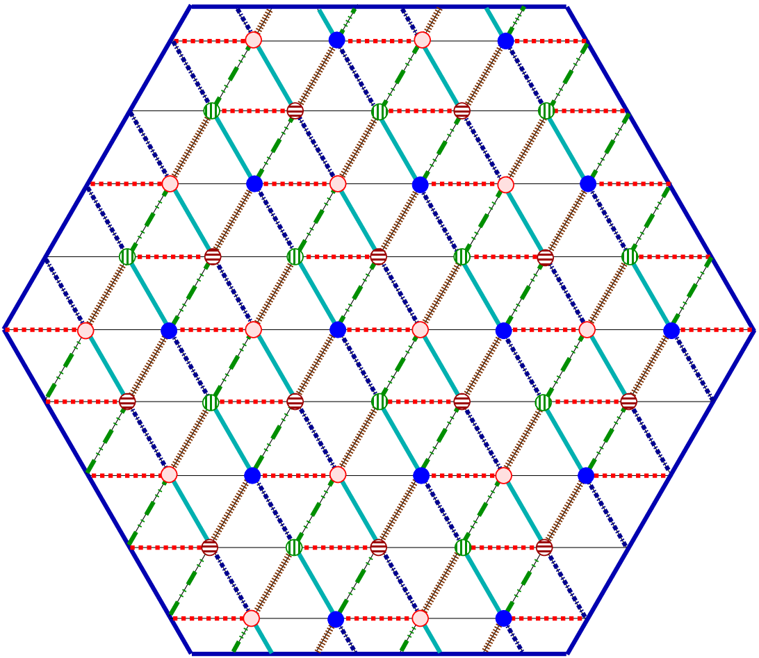
This model can also represent a tri-layer system with plaquette interactions.
One can indeed realize that there is nothing special about the Lie algebra so. One can consider models whose bond algebra forms any other semisimple Lie algebra, such as so where there are non-linear Bogoliubov transformations that diagonalize the problem. It is important, though, that the number of gauge symmetries is enough to allow for a simple oscillator realization of the bonds. Otherwise, there is always the possibility to use the Jacobi algorithm [3] to numerically diagonalize the problem.
V Conclusions
The thesis of the current work is that even though the solution to many problems is hard, by disregarding the explicit microscopic degrees of freedom and focusing solely on the algebraic relations that the bond variables satisfy in a Hilbert space of a fixed dimensionality, we may map one initially seemingly hard problem onto another problem whose solution is easier. This mapping does not rely on explicit real space forms for the transformations (although these can be written down in some cases). Nor does it rely on enlarging the Hilbert space and then making a projection onto a physical sector as in [20]. It is important to emphasize, though, that the dimension of the representation of the algebra is of crucial importance - not only the algebra and set of constraints itself.
The explicit real space mappings – no matter how complicated their forms are – are irrelevant. The spectra and all non-vanishing correlators may be determined from the algebra alone. [See [8] for a derivation of all correlators in Kitaev’s Toric code model by this method.] In the current work, we illustrated how the energy spectra may be determined. The partition function and the density of states associated with the spectrum are related by a Laplace transform. It may be easily seen also from the partition functions themselves that if two systems display the same bond algebra on a space of the same representation then their spectra are identical.
In the case of generic GMFHs the Jacobi method always enables a solution of its spectrum with polynomial complexity [3]. There are situations, like the model examples presented in this paper, where we can determine the spectrum of certain sectors (Hilbert subspaces) in closed form, i.e., by quadrature. This will happen whenever the effective matrices that need to be diagonalized have dimension smaller or equal to 4 . The decomposition of the Hilbert space into these individual decoupled subspaces is rooted in the existence of local (gauge) symmetries. Within each subspace, there is an oscillator realization (e.g., in terms of Majorana fermions) of the bond algebra. It is important to emphasize that exact solvability does not imply that we can compute the density of states, and thus the partition function, with polynomial complexity. Kitaev’s honeycomb model is an example of a system whose energy eigenvalues can be determined with polynomial complexity but whose total partition function cannot since its density of states is not determined with the same complexity. By contrast, Kitaev’s Toric code model constitutes an example of a system where not only the spectrum but also its partition function is exactly solvable [7, 8].
Note added in proof. This work (and our vector-exchange model) was conceived in 2007. A physical model whose exact solution was enabled by our bond algebra mapping is detailed in [1]. During the time in which the current work was summarized, three works appeared [24, 25, 29] that introduce and solve variants and exact forms of the vector-exchange model that we introduced here. In particular, [25] presented a spin system and the vector-exchange model on the Shastry-Sutherland [28] decorated square lattice.
References
- [1] Z. Nussinov and G. Ortiz, Europhysics Letters 84, 36005 (2008).
- [2] X-G. Wen, Quantum Field Theory of Many-Body Systems (Oxford University Press, Oxford, 2004), and references therein.
- [3] R. Somma, H. Barnum, G. Ortiz, and E. Knill, Phys. Rev. Lett. 97, 190501 (2006).
- [4] W. Brzezicki, J. Dziarmaga, and A. M. Oles, Phys. Rev. B 75, 134415 (2007).
- [5] A. Kitaev, Ann. Phys. 303, 2 (2003).
- [6] M. Mézard, G. Parisi, and M.A. Virasoro, Spin glass theory and beyond (World Scientific, Singapore, 1987).
- [7] Z. Nussinov and G. Ortiz, cond-mat/0605316.
- [8] Z. Nussinov and G. Ortiz, cond-mat/0702377v5 (2007).
- [9] Z. Nussinov and G. Ortiz, Phys. Rev. B 77, 064302 (2008).
- [10] X.G. Wen, Phys. Rev. Lett. 90, 016803 (2003).
- [11]
It is important to note that all of the steps invoked in the
high-temperature expansion discussed below rely only on the operator
algebra and the dimension of its representation. First, note that
.
Then, the partition function is
with all graphs on the lattice (subset of lattice sites). The graph spans sites and plaquettes. As and , and as the trace of any Pauli matrix raised to an odd power is zero, the only terms surviving in the sum of Eq.(90) are those with graphs such that each lattice link appears in an even number of star operators (i.e., zero or two) and an even number of plaquettes (zero or two). The trace over these non-vanishing terms is , as there are possible bond configurations (and a total of bonds) and raised to an even power is the identity operator. The only graphs on a torus that satisfy this condition are those in which (i) is the empty set, (ii) contains all stars in the lattice, (iii) contains all plaquettes in the lattice, or (iv) contains all stars and plaquettes in the lattice. These give rise to finite terms as the products over the entire torus, and , by virtue of the topology (each bond on a square lattice on a torus appears in an even number of plaquettes or stars). Summing up these four graphs we have, Eq.(19).(90) - [12] A. Kay and R. Colbeck, arXiv:0810.3557.
- [13] R. Alicki, M. Fannes, and M. Horodecki, arXiv:0810.4584.
- [14] R. Alicki, M. Fannes, and M. Horodecki, arXiv:quant-ph/0702102, J. Phys. A: Math. Theor. 40, 6451 (2007).
- [15] S. Bravyi and B. Terhal, arXiv:0810.1983.
- [16]
As a curiosity, it is worth noting that our bond algebraic mapping gives
rise to a crossover for finite size systems. As we showed by the
application of bond algebras, Kitaev’s Toric code model is isomorphic
to two decoupled Ising chains. The correlation length within an Ising
chain of exchange constant as in Eq.(18) is given by
When , the system may appear to be ordered while for , the system is disordered across the chain. When , the function(91)
Consequently, the crossover temperature at which is given by(92)
For the system may support instantaneous local order across a finite size system. As , the crossover temperature tends to zero. The existence of a crossover temperature with a scaling that we derived here (Eq.(93)) from our old bond algebra mapping to a one-dimensional system [7, 8] coincides with that seen in the entanglement entropy [17]. Related scalings for mutual information were derived in [18].(93) - [17] C. Castelnovo and C. Chamon, arXiv:0704.3616, Phys. Rev. B 76, 184442 (2007).
- [18] S. Iblisdir, D. Perez-Garcia, M. Aguado, and J. Pachos, arXiv:0806.1853.
- [19] J. Yu, S-P. Kou, and X-G. Wen, arXiv: 0709.2276.
- [20] A. Yu. Kitaev, Ann. Phys. 321, 2 (2006).
- [21] H-D. Chen and Z . Nussinov, J. Phys. A: Math. Theor. 41 075001 (2008).
- [22] J. K. Pachos, Annals of Physics, 322, 1254 (2007); G. Baskaran, D. Sen, and R. Shankar, Phys. Rev. B 78, 115116 (2008); S. Mondal, D. Sen, and K. Sengupta, Phys. Rev. B 78, 045101 (2008); S. Dusuel, K. P. Schmidt, J. Vidal, Phys. Rev. Lett. 100, 177204 (2008); S. Dusuel, K. P. Schmidt, J. Vidal, and R. L. Zaffino, Phys. Rev. B 78, 125102 (2008); J. Vidal, K. P. Schmidt, S. Dusuel, arXiv:0809.1553.
- [23] D. F. Abasto and P. Zanardi, arXiv:0809.4740.
- [24] H. Yao, S-C. Zhang, and S. A. Kivelson, arXiv: 0810.5347 (2008).
- [25] C. Wu, D. Arovas, and H-H. Hung, arXiv:0811.1380 (2008).
- [26] S. Elitzur, Phys. Rev. D 12, 3978 (1975).
- [27] G. Baskaran, S. Mandal, and R. Shankar, Phys. Rev. Lett. 98, 247201 (2007).
- [28] S. Shastry and B. Sutherland, Physica B and C 108, 1069 (1981).
- [29] S. Ryu, arXiv:0811.2036.