Constraints on amplitudes of curvature perturbations from
primordial black holes
Abstract
We calculate the primordial black hole (PBH) mass spectrum produced from a collapse of the primordial density fluctuations in the early Universe using, as an input, several theoretical models giving the curvature perturbation power spectra with large () values at some scale of comoving wave numbers . In the calculation we take into account the explicit dependence of gravitational (Bardeen) potential on time. Using the PBH mass spectra, we further calculate the neutrino and photon energy spectra in extragalactic space from evaporation of light PBHs, and the energy density fraction contained in PBHs today (for heavier PBHs). We obtain the constraints on the model parameters using available experimental data (including data on neutrino and photon cosmic backgrounds). We briefly discuss the possibility that the observed 511 keV line from the Galactic center is produced by annihilation of positrons evaporated by PBHs.
pacs
98.80.-k, 04.70.-sI Introduction
It is well known that for a sufficient production of primordial black holes (PBHs) in the early Universe [1, 2, 3, 4] the spectrum of the density perturbations set down by inflation must be “blue”, i.e., it must have more power on small scales. This implies that the spectral index of the scalar perturbations must be larger than 1, in strong contradiction with the latest WMAP results [5, 6, 7]. In particular, standard inflationary models of hybrid type, in which the inflaton is trapped in a local minimum of the potential and which predict blue spectra seem to be excluded as a possible source of PBHs.
Such a conclusion is correct, however, only in rather special case: namely, it is based on the prediction of slow-roll single field inflationary scenario, according to which the power spectrum of curvature perturbations is nearly scale-invariant, i.e., the spectral index is close to unity and the variation in the spectral index is small.
Although a prediction of the approximate scale invariance of the primordial power spectrum is a necessary requirement to any inflationary model, some deviations from pure scale invariance are consistent with the observational data. These deviations are described by adding localized features to the primordial spectrum (see, e.g., [8] and references therein) and/or by introducing spectral features modifying a single power law. Models with such peculiarities (sometimes called broken-scale-invariant (BSI) models) were proposed, in main aspects, in eighties [9, 10, 11, 12, 13, 14]. Such models generally include, in addition to the usual inflaton field, other scalar fields driving successive stages of inflation and triggering phase transitions.
Evidently, the BSI models of inflation could predict, generically, the essential production of primordial black holes at small and medium scales. In particular, in [15] the inflationary model with a steplike power spectrum based on a nonanalyticity in the inflaton potential was proposed and in subsequent works the inflationary potentials of such kind were used for making predictions of PBH production [16, 17, 18].
A step feature in the potential is an effective field theory description of a phase transition, so, in a more realistic approach an inflationary model should certainly involve more than one scalar field, and such rapid phenomena as phase transitions [19]. Second order phase transitions during inflationary expansion had been first considered in [11, 13] in models with two scalar fields. In scenarios of such type, during a short stage, corresponding to the beginning of a phase transition, the mass of the trigger field becomes negative, and adiabatic perturbations are exponentially amplified resulting in the formation of a narrow spike in the primordial spectrum, and, as a consequence, in a copious production of PBHs [20, 21]. There are many multiple field scenarios predicting the existence of spike- or bumplike features in the primordial spectrum (e.g., supersymmetric double hybrid models [22], multiple inflation models based on supergravity [23], etc). Some of these models are specially constructed to predict efficient PBH production [24, 25].
Further, large curvature perturbations (especially on subhorizon scales) leading to features in the primordial spectrum and possible PBH production, can arise in multiple field scenarios at the end of inflation (during preheating era) or between two consecutive stages of inflation, as a result of parametric resonance or tachyonic instability. Estimates of PBH production possibilities had been obtained in [26, 27, 28] for two-field models and in [29] for models with a self-interacting scalar field. The more complicated model (containing three fields), based on supergravity, is considered in [25].
An existence of the narrow spikes in the primordial spectrum is possible not only in multiple field inflationary scenarios. Such a feature can, in principle, exist even in single field models (see, e.g., [30, 31]). If, in particular, the inflationary potential has an unstable maximum at origin (e.g., the double-well potential) then, with some fine-tuning of parameters and initial conditions, the inflation process may have two stages, with a temporary stay at the maximum, that may lead to the corresponding peak in the primordial spectrum and, depending on the amplitude of the peak, to the PBH production.
Another example of an inflationary model predicting large amplitudes of the density perturbations at small scales is the inflationary model with the running mass potential. More generally, large amplitudes of the primordial curvature perturbation spectrum at small scales are possible in models of ”hilltop hybrid inflation” [32]. Potentials of these models have concave-downward form at cosmological scales (corresponding to red primordial spectrum as required by observations), but can be much flatter near the end of inflation. Such a modification of a standard hybrid inflation scenario is discussed, e.g., in [33, 34]. The running mass potential belongs to the class of hilltop potentials; in models with such potentials, due to spectral index scale-dependence, the amplitude of the perturbation spectrum at small scales depends on the value of at cosmological scales [32]. It is shown in our previous work [31] that possibilities of noticeable production of PBHs in running mass model are still open in spite of the rather severe experimental constraints [35, 36] on the value of the spectral index running.
In this paper we limit ourselves to the situations where PBHs form from the density perturbations, induced by quantum vacuum fluctuations during inflationary expansion. The details of the PBH formation had been studied in [37, 38], the astrophysical and cosmological constraints on the PBH density had been obtained in many subsequent works (see, e.g., the recent review [4]). The order of magnitude of the corresponding constraint on the value of the density perturbation amplitude (for the PBH mass region g, which we are interested in) is well known [39], but, if the primordial spectrum contains the peaklike feature, the concrete value of the PBH constraint clearly depends on the parameters characterizing the form of this feature (in particular, on the width of the peak). Such an information may be rather useful for the model makers.
One must note that the formation of PBHs in models with the primordial spectrum having the features had been studied earlier, in works [40, 41]. In [40] the case of the spectrum that is sharply peaked on a single mass scale was considered. The function (the probability of a region of mass to form a PBH) was calculated and it was shown that the form of this function depends on the type of the gravitational collapse. In [41] two cases were studied: a pure step in the primordial spectrum and the spectrum produced in an inflationary model [15] with a jump in a first derivative of the inflaton potential at some scale. It was shown that the corresponding -functions have the pronounced bumps and, in connection with these bumps, authors of [41] discuss the possibility that PBHs can be a significant part of dark matter.
In the present work we reconsider the problem of constraining the power spectrum of the primordial fluctuations (with accent on the peaklike features) calculating the process of the formation of PBHs having small masses (g). Products of evaporation of these PBHs contribute, in particular, to extragalactic photon and neutrino diffuse backgrounds (which are measured experimentally), and the constraints are calculated using the standard procedure [42]. We do not calculate the -functions preferring to constrain the power spectrum directly. The concrete constraints are obtained for two special cases (the power spectrum with a peak and the spectrum of the running mass model), although the general formulas of Sec. II and III can be used for any form of the spectrum.
At the end of the paper we use our approach for a checking, once more, the idea proposed in [43, 44], namely, we study the possibility that evaporating PBHs (having mass spectrum calculated with formulas of Sec. II) cluster in the Galactic center and produce the observed keV photon line.
The plan of the paper is as follows. In Sec. II we present the general formalism of the PBH mass spectrum calculation with taking into account the explicit time dependence of the gravitational potential. The results of such a calculation for the concrete example, in which the curvature perturbation spectrum has a sharp peak, are given. In Sec. III we give some details of the calculation of the neutrino and the photon extragalactic diffuse spectra from the PBH evaporations. In Sec. IV and Sec. V the constraints on the curvature spectrum from PBHs are given, for the model of with a peak and for the running mass model, respectively. In Sec. VI we consider the possibility of the explaining the observed keV photon line from the Galactic center by PBHs clusterizing there. Section VII contains our conclusions.
II PBH mass spectrum calculation
II.1 General formula
The calculation of PBH mass spectrum in Press-Schechter formalism [45] is based on the expressions [46, 47, 48]
| (1) | |||
| (2) |
Here, the following notations are used: is the initial density contrast smoothed on the comoving scale , is the smoothing mass, is the mean square deviation (the mass variance),
| (3) |
is the power spectrum of primordial density perturbations, is the Fourier transform of the window function (in this work we use the gaussian one, ), is the initial energy density. It is assumed that the process of reheating is very short in time, so, the end of inflation practically coincides with a start (at ) of the radiation era.
Fourier transform of the (comoving) density contrast is
| (4) |
where is the Fourier transform of the Bardeen potential. In the approximation , we have, for the radiation dominated epoch, , that is the well-known result [49]. In this work, however, we will not use this approximation and, in opposite, we will explicitly take into account the time dependence of the Bardeen potential.
The power spectrum of the density perturbations, calculated at some moment of time, is
| (5) |
where is the conformal time ( for the radiation epoch).
The comoving smoothing scale, , is connected with the smoothing mass by the expression
| (6) |
where , and are the horizon mass, cosmic scale factor and Hubble parameter at the moment . Eq. (6) immediately comes from two simple formulas: horizon mass at is given by
| (7) |
and the smoothing mass is
| (8) |
From these relations, one obtains
| (9) |
and putting we come to Eq. (6).
For the practical use of formulas (1, 2) one must express the PBH mass through the smoothing mass and the density contrast at the moment of the collapse (which is approximately equal to the density contrast at horizon crossing, ).
It follows from Eq. (4) that the smoothed density contrast at the initial moment of time, , and at the time of horizon crossing, , are connected by the expression
| (10) |
Here we use the approximation according to which the smoothed density contrast is proportional to its Fourier transform at some characteristic value of , . If the power spectrum increases monotonically with , then, evidently, . If the spectrum has a maximum at some value of , , the reasonable estimate for is
II.2 Gravitational collapse models
The connection between values of the smoothing mass , density contrast and PBH mass can be expressed in the general form
| (14) |
The concrete expression for the function depends on the model of the gravitational collapse. In the model of the standard spherically-symmetric collapse the connection is quite simple:
| (15) |
Here, is the horizon mass at the moment of time, , when regions of the comoving size and smoothing mass cross horizon. According to Carr and Hawking [50], . The derivation of Eq. (15) is given in the Appendix A.
The horizon mass at the moment when a region of the comoving size crosses horizon is
| (16) |
(at this moment, ). Using (7), one obtains
| (17) |
Finally, using (6), the connection between and is derived [48]:
| (18) |
This equation connects horizon mass at the moment of time when the perturbed region crosses horizon with the initial (at ) horizon mass and the initial (at ) comoving mass . It is seen that the comoving mass decreases with time () (see, e.g., [51]).
In the picture of the critical collapse [52] the corresponding function is
| (20) |
where , and are model parameters. In this work we will accept the following set of parameters, which is in agreement with the recent calculations [53, 54]:
| (21) |
One should note that the neglect of a time dependence of the gravitational potential greatly simplifies a calculation of the PBH mass spectrum because the smoothed density contrast enters the PBH mass spectrum expression only through the ratio . In the limit of the constant one has, from Eqs. (18) and (6),
| (22) |
In the same limit, an expression for the mass variance is
| (23) |
It follows from Eqs. (22) and (23) that
| (24) |
This ratio is constant with time. It is clear from these arguments that a time dependence of (given, e.g., in Fig. 1) will affect the form of the PBH mass spectrum (see Sec. V).
II.3 Time dependence of the gravitational potential
For a calculation of a time dependence of the gravitational potential we use the approach suggested in works of Ref. [55]. We assume that reheating is rapid and, correspondingly, the moment of the end of inflation coincides with the moment of a beginning of the radiation epoch. The only difference from the consideration of [55] is that we do not assume, in general, the validity of the slow-roll approximation at the period near the end of inflation.
The general expression for the Fourier transform of the Bardeen potential at the radiation epoch is
| (25) |
| (26) |
| (27) |
where , is the sound speed. The connection between and Fourier components of the curvature perturbation in gauge invariant cosmological perturbation theory is given by two expressions (see, e.g., the review [56]):
| (28) |
| (29) |
For obtaining the coefficients , we need two conditions for . The first one is the Eq. (28) calculated for the end of inflation, when , , , and . The second one is the Eq. (29) calculated for the beginning of the radiation era when , , and . The junction conditions at the transition time are [[57], [58], [55]]:
| (30) |
| (31) |
Using Eqs. (28, 29) and (30, 31), one obtains for the coefficients , the following two conditions:
| (32) |
| (33) |
Two inputs in these expressions, and , can be determined by a numerical calculation (see, e.g., [31]) using the concrete inflation model.
In the present paper, we assume, for simplicity, that the right-hand side (rhs) of Eq. (32) is equal to zero. It does not mean, however, that we exclude a consideration of non-slow-roll models because the rhs of Eq. (32) contains, except of the term , also the time derivative of which is typically small due to freezing out of outside of horizon (if the comoving size crosses horizon some time before the end of inflation, see, e.g., [31]). The general case when violations of slow-roll are continuing up to the end of inflation (and when, correspondingly, the rhs of Eq. (32) cannot be neglected) will be considered in a separate paper.
As a consequence, is proportional to , and one has, instead of Eq. (5), the simple connection between density perturbation at any time and curvature perturbation at initial moment of time
| (34) |
where the expression for is given by [55]
| (35) |
Correspondingly, in this approximation only one input value, , is needed for a calculation of the Bardeen potential.
In Fig. 1 typical results of the calculation using Eqs. (35) and (4) are shown. It is clearly seen from the figure that in our approximate approach (instantaneous transition from inflation to the radiation era) the evolution of the Fourier transform of the density contrast starts from zero value. In practical calculations of PBH production we displace the starting moment from to ignoring this production inside the short time interval . Specifically, the shift was determined by the condition , throughout all numerical calculations.


II.4 Power spectrum with maximum
One of scenarios in which significant PBH production is possible is the one with the power spectrum having a strong bump near some value in the region of small scales. Such models have been considered in many papers, including [16, 20, 21, 24, 25, 30, 31].
Having the exact form of the power spectrum , it is possible to calculate the PBH mass distribution using the formalism introduced in the previous sections. However, to be more general, it is convenient to introduce some parametrization of , and use it to calculate PBH mass spectra. For example, we find that power spectra with peaks considered in [31] can be rather well parameterized in the region of the maximum with a distribution of the form
| (36) |
(it is similar to the primordial spectrum parametrization used in [59] and in our previous work [60]). Here, the value of is known from observations at large scales (), and its exact value does not affect the PBH production rate. is the maximum value approached by the power spectrum, and are parameters determining the position and width of the peak.

It is clear that any power spectrum with maximum can be more or less well approximated in the most important region (near the maximum) just by three parameters, determining the position of the peak, its height and width. Thus, the results from taking the spectrum in such a form will be quite general, because PBH production is mostly determined, of course, by the region of the spectrum near the maximum.
The connection between the wave number and horizon mass at the moment when the mode enters the horizon is determined from (6) and (18) and is
| (37) |
and further we will use a notation , which is the horizon mass corresponding to a value of .
The result of PBH mass spectrum calculations with the particular set of parameters is shown in Fig. 2. It is seen that the mass spectrum strongly depends on the model of the gravitational collapse (at the same values of the fluctuation spectrum parameters). One should note that on this and some following figures we show on the vertical axis the quantity , which is the comoving number density of PBHs, and is independent on the reheating temperature in the limit . The case when values of are important for the PBH production will be discussed in Sec. V.

Figure 3 shows a dependence of the PBH mass spectrum on the parameter in Eq. (36). We can see that this dependence is rather strong, that comes from the fact that has an exponential sensitivity to the mass variance (which, in turn, is determined by the shape of the spectrum, including its width). We also see that the mass spectrum is always rather strongly peaked near the PBH mass .
The fraction of an energy density of the Universe contained in PBHs today, , assuming that a mass of the produced black hole does not change in time, is
| (38) |
( is the critical density). This formula is rather accurate for black holes with initial mass , where g is the initial mass of PBH which reaches its final state of evaporation today [61], , and is the age of the Universe.
One should note that for the concrete PBH mass spectra shown in Fig. 3, we have, for the case of , the inequality , which is an inconsistent result, so the production of such a big amount of PBHs is forbidden. We will discuss the possibility of a constraining the model parameters in the distribution of Eq. (36) in detail further, in Sec. IV. The value chosen for the calculation of the spectra shown in Fig. 3 corresponds, in the case of , to the value equal to . This is in the range needed to explain the observed amount of non-baryonic dark matter [62], (with uncertainty). For the case of , it appears that , probably too small of a fraction to produce observable cosmological consequences.
III Neutrino and photon spectra from PBHs evaporations
PBH evaporation, predicted by Hawking [63], causes evaporating black holes to produce an isotropic extragalactic photon and neutrino backgrounds, which can be, at least in principle, measured experimentally. It can be calculated having the PBH mass spectrum, and the comparison with observations can be made.
Evolution of a PBH mass spectrum due to the evaporation leads to the approximate expression for this spectrum at any moment of time:
| (39) |
where accounts for the degrees of freedom of evaporated particles and, strictly speaking, is a function of a running value of the PBH mass . In our numerical calculations we use the approximation
| (40) |
where is the value of in the initial mass spectrum corresponding to a maximum of this spectrum. Special study shows that errors connected with such an approximation are rather small. In this work we use parametrization of the function presented in [48].
The expression for the extragalactic differential energy spectrum of neutrinos or photons (the total contribution of all black holes) integrated over time is [48]
| (41) | |||
In this formula, , , and are cosmic scale factors at , and at present time, respectively, and is a total instantaneous spectrum of the radiation (neutrinos or photons) from an evaporation of the individual black hole. The exponential factor in Eq. (41) takes into account an absorption of the radiation during its propagation in space. The processes of neutrino absorption are considered, in a given context, in [48]. In the last line of (41) we changed the variable on red shift using the flat cosmological model with for which
| (42) |
(, ), with the set of the basic cosmological parameters taken from [62]: , , , . The neutrino fraction in the total energy density, , is calculated assuming that the neutrino masses are negligible, in this case (the term with is essential in Eq. (42) only for ).

The direct Hawking flux of evaporated particles (per degree of freedom) is
| (43) |
where is a grey-body factor ( for massless particles, where is the absorption cross section), and is the Hawking temperature
| (44) |
In the high energy limit (), the cross section approaches a constant value independent of , and in this case is
| (45) |
For lower energies, however, this factor needs to be calculated numerically.
For photons, we use the following approximate parametrization of this function [64]
Here, the low-energy part comes from analytically obtained relation [61] ( is the Schwarzschild radius). The higher energy part is just an approximation smoothing the oscillations in , see Fig. 4. The form of Eq. (III) at high energies is analogous to one used in [65] for neutrinos,
| (50) |
The instantaneous spectra of neutrinos and photons from PBH evaporations were calculated using the model of Ref. [66] and parametrization of Ref. [67]. In these papers the particles directly emitted from the black hole (through the Hawking mechanism) as well as those produced in processes of quark fragmentations and subsequent decays of mesons had been taken into account.

In Fig. 5 the red shift distributions of the differential energy spectra are shown for the neutrino or photon with energy 1 GeV. One can see that the distributions are more wide in the case of the critical collapse (because the PBH mass spectrum in this case has a long ”tail” of small masses). The absorption factor is efficient: in case of photons, the maximum value of for which the absorption can be neglected is around [68]; for neutrinos the absorption is important at [48].
IV Constraints on the power spectrum with maximum
Assuming that has the form of Eq. (36), we can calculate the produced PBH mass spectra, compare the possible consequences of the existence of such amount of PBHs with observations, and put limits on the parameters of this distribution. The calculation of the actual constraints in this paper (as well as in our previous work [60]) uses the following basic observational facts.
1. The differential energy spectrum of the extragalactic photon background in the wide region of energies is known [69]. For our purpose, the most interesting range is about MeV GeV, and the order of magnitude of the flux is roughly given by GeV cm-2 s-1 sr-1 in this region. We obtain our constraints just from the condition that the diffuse gamma ray flux produced by PBHs does not exceed the observed extragalactic one.
2. According to the data of Super-Kamiokande experiment [70], the electron antineutrino background flux in extragalactic space is constrained by the inequality
| (51) |
We integrate the calculated flux and put constraints from the condition that it does not exceed this limit. We note, however, that the limit (51) is not a model-independent one. It was obtained assuming exponentially falling neutrino spectrum, which is an expectation for the extragalactic diffuse flux from supernovae. The neutrino flux from PBHs in the mass region we consider is falling as , which, in fact, will change the constraint (51). Estimations show, however, that this change is about a factor of 2, and it is not very significant for putting constraints on such parameters as . Similar uncertainty also comes from the inclusion of neutrino oscillations in the analysis, which we do not take into account.
3. The fraction of the energy density of the Universe contained in PBHs, , which can be calculated using formula (38), cannot exceed the one for non-baryonic dark matter, [62]. This constraint is important for black holes with initial mass , i.e., ones that did not evaporate up to the present time.
The actual condition we use is (having all the uncertainties considered, is still allowed by the observations within the confidence interval, however, the uncertainty in this number does not seriously affect the power spectrum constraint).

The resulting constraints obtained from all the conditions discussed are shown in Fig. 6. The value of the parameter characterizing the width of the gaussian distribution in Eq. (36) was fixed throughout all calculations (). The constraints are given as a function of the horizon mass . The connection of with the corresponding wave number is very simple and is given by the formula following from Eq. (37):
| (52) |
It follows from these results that the constraints are stronger under assumption of the standard Carr-Hawking collapse, which is expected because in this case the threshold density contrast leading to PBH formation is smaller. The constraints are independent on the reheating temperature if it is high enough to provide the condition (this is true for all PBH masses considered if GeV).
The second important result is that the constraints based on the neutrino emission of PBHs are comparable with those following from the photon emission and from the gravitational constraint. At the region of small horizon masses (large ), where large red shifts are important, the constraints from the neutrino emission are stronger.
Fig. 6 is analogous to one presented in our previous work [60]. In the present paper we add the gravitational constraint on and more carefully investigate the mass region g. In this region, constraints from energy density and from gamma ray background coexist. We do not extend in the present paper the neutrino constraints to masses because the neutrino background in this case strongly deviates from the simple behavior and additional analysis is needed to estimate how the limit of Eq. (51) will change in such a situation.
V Constraints on the running mass model from PBHs
The running mass inflation model was proposed in [71, 72] and further studied in many papers including [74, 73, 75, 76, 77]. The model predicts a rather strong scale dependence of the spectral index, possibly allowing large values of at small scales, which can lead to PBH production [[78], [79], [31]]. The first constraints on the running mass model parameters from PBHs were obtained in works [78, 79]. In previous works the PBH mass spectrum in the running mass model have not been calculated in detail. We do it in the present paper to demonstrate how the general formalism developed in Sec. II works.
We will also show how it is possible to constrain such observable parameters as the spectral index measured at cosmological scales, , and its running , assuming the running mass model is correct.

The potential of the running mass model takes into account quantum corrections in the context of the softly broken global supersymmetry and is given by the formula
| (53) |
The dependence of the inflaton mass on renormalization scale is determined by the renormalization group equation (RGE).


Apart from , the shape of the running mass potential is determined by parameters and , which are connected to the other quantities by
| (54) | |||
| (55) |
(, and is the value of the inflaton field corresponding to the cosmological scale ). They are also linked to observables and :
| (56) |
and we see that measuring and allows us to reconstruct the potential shape in this model, and the only free parameter left is (or ). From the theoretical point of view [77], can lie in the wide range of values from, say, GeV for anomaly-mediation case to GeV for gauge-mediation. Assuming instant reheating at some value of the inflaton field, from the energy conservation condition we have:
| (57) |
(), and the reheat temperature turns out to be in the region GeV for the given values of . For further calculation we will use two values of , namely, and GeV.
It was noted in [31], that for the running mass model, the numerical calculation of the power spectrum is necessary in the region of large values. In this work we also use the numerical calculation of power spectra, not relying on the analytical approximations. Several results for are given in Fig. 7, which shows how sensitive is the value of near the end of inflation to the change in .
Some examples of the PBH mass spectrum calculation are given in Fig. 8 for two models of the collapse considered above. The order of magnitude of the PBH mass produced is equal to the initial horizon mass , which is given by
| (58) |
The real PBH mass spectrum, and, particularly, its maximum, is, however, determined by the dynamics of their formation, including the dependence of the gravitational potential on time. This dependence is very important in the region of smallest possible PBH masses produced, i.e., in the case . For example, in the model of the standard collapse with a monotonous power spectrum we would expect most of PBHs to be produced near the smallest possible mass, i.e., near (e.g., g for GeV). From Fig. 8 we see, however, that the actual maximum is near g in this case, which is due to suppression of PBH production at smaller masses.

Fig. 9 shows the constraints on obtained assuming that the running mass model is correct. Reconstructing the potential from values of , and , we calculate the power spectrum in the whole region of wave numbers up to , and the corresponding PBH mass spectrum. The method of obtaining the constraints depends on the characteristic PBH mass produced: for GeV, the PBH mass in maximum of the distribution is about g (see Fig. 8), and neutrino background data was used to constrain such models, because, as we have seen in Sec. IV, neutrino experiments are adequate to constrain PBHs of such initial masses. For GeV, the PBH mass in maximum of the spectrum is about g, and constraints are obtained using the extragalactic gamma ray background.
We see from Fig. 9 that, assuming running mass model is really responsible for inflation and production of perturbation spectrum, running of the spectral index at cosmological scales is strongly constrained by PBH overproduction and cannot be larger than (the exact value of the constraint depends on other parameters).
VI Dark matter and PBHs
PBHs produced in the early Universe, if they are heavy enough not to evaporate till the present day, can contribute to dark matter, and potentially it is possible to explain all the non-baryonic dark matter with them. For example, the mass spectrum shown in Fig. 3 (for the case of ) gives .
In works [43, 44], PBHs clustered in the Galactic bulge are proposed to explain the observed keV photon line from the Galactic center [80, 81]. Positrons evaporated from PBHs annihilate with electrons from the interstellar medium thus producing the observed photons. Assuming that Solar System lies at a distance of kpc from the Galactic center, the total positron production rate needs to be about s-1, and the corresponding characteristic value of the PBH mass should be in the range g (this was shown in ref. [44] from calculations of the photon background in extragalactic space and the photon flux from the Galactic center from PBH evaporations). We will show in this paper that our distribution presented in Fig. 3 (for ) is also capable to explain the needed positron production rate.

Assuming that the PBH mass distribution in Galaxy does not change compared to the initial one, for the PBH mass distribution in the Galactic center we can write a simple proportionality relation
| (59) |
where will be determined by the total mass of PBHs:
| (60) |
The gamma ray flux on the Earth surface produced by such PBHs is
| (61) | |||
and the positron production rate in the Galactic center is
| (62) | |||
The total mass needed can be expressed through the observable positron production rate and the initial mass spectrum by the formula
| (63) |
In our case, we obtain . If these black holes are uniformly distributed in the spherical region of radius pc, the clusterization factor needed for that is about
| (64) |
The gamma ray flux from such PBHs calculated using Eq. (61) is presented in Fig. 10, together with the measured continuum, given by the approximate formula [81, 44]
| (65) |
and we see that the flux from PBHs does not exceed the observational one.
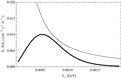
For the calculation of diffuse extragalactic photon flux, clusterization of PBHs is not important, because this flux is sensitive to the average number of PBHs and their mass distribution only. Thus, formula (41) is suitable for the calculation. It can, however, be much simplified because such PBHs (with mass sufficiently larger than ) do not lose the significant part of their mass in course of the evaporation, and approximation is adequate, so we can neglect the quantity in it. The absorption factor can also be dropped because the effectively working red shifts in this task are small. The diffuse gamma ray flux from our PBH mass distribution (Fig. 3, ) is shown in Fig. 11. We see that, again, the experimentally measured flux, given by [69, 44]
| (66) |
is not exceeded.
VII Conclusions
1. We have developed a method of PBH mass spectrum calculation, which is based on the Press-Schechter formalism and takes into account the dependence of the gravitational potential on time. We found that it is more convenient and natural to use in the formula for the mass variance (Eq. (3)) the gravitational potential calculated as a function of time rather than the transfer function (the latter is defined, e.g., in [41]). To derive the PBH mass spectrum, the power spectrum of curvature perturbations calculated (using inflationary models) at the end of inflation is needed as an input.
2. PBH mass spectra are calculated in two inflationary models predicting large amplitudes of the curvature perturbation spectrum at some wave number , namely, in the model with the power spectrum with a peak and in the running mass model. Examples of such a calculation are given in Figs. 2, 3 and 8.
3. Constraints on parameters of both these models are obtained using available data on the extragalactic photon diffuse background and the upper limit on the extragalactic neutrino background, obtained in the Super-Kamiokande neutrino experiment.
The results are shown in Figs. 6 and 9. It is seen that for the power spectrum with a peak, the height and the width of the peak can be constrained in rather wide region of wave numbers determining its position in the spectrum. For the running mass model we obtain the constraint on the spectral index running at cosmological scales, (the exact constraint value depends on and ).
4. It follows from Fig. 6 that constraints obtained from neutrino experiments are stronger than those obtained from extragalactic photon background, in the region of horizon masses from to g. So, constraints from neutrino experiments and from measurements of diffuse photon background are complementary.
5. PBHs can be the main contributor to the dark matter in the Universe. It is shown that if, in this case, the PBH mass distribution is peaked near g, as in Fig. 3 with , the experimentally observed galactic keV photon line can, in fact, be caused by annihilating positrons produced by evaporating PBHs clustered in the Galactic center. The total PBH mass needed for this to happen must be about , and clusterization factor needed is .
Acknowledgements.
The authors are grateful to Professor A.A. Starobinsky for the important remark. The work was supported by Russian Foundation for Basic Research (Grant No. 06-02-16135).Appendix A Formation of PBHs in a radiation-dominated universe
In this Appendix we give basic formulas of the PBH formation process following closely the work [18].
Evolution of a spherically symmetric region with density greater than the background density is governed by the positive curvature Friedmann equation,
| (67) |
Here, , and are Hubble parameter, density and a physical size of the region, respectively. In a background space the evolution equation is, correspondingly,
| (68) |
An expansion of the overdensed region goes on according to the law [82]
| (69) |
and stops at time . This time is determined from the condition and is given by the expressions
| (70) |
where is the initial moment of time (which is chosen in such a way that [18]). This should not be confused with of Sec. II. The size of the region at is
| (71) |
The perturbed region will contract and, eventually, collapse, if it contains enough matter to get over pressure forces, i.e., if its radius exceeds the Jeans length,
| (72) |
The corresponding requirement for the PBH formation is
| (73) |
(the value of the upper bound is explained in [[50], [37]]). Dividing (73) by , we obtain the expression for ,
| (74) |
which scales, approximately, like a constant (independent on time) because
| (75) |
Evaluating (74) at horizon crossing (where ), we obtain from (73) the necessary condition for the collapse (and the PBH formation)
| (76) |
Here we used the notation for the density contrast at horizon crossing introduced in Sec. II.
The mass of a black hole formed in a process of the collapse is given by
| (77) |
| (78) |
| (79) |
Substituting (78) and (79) to (77), one obtains
| (80) |
References
- [1] Ya. B. Zeldovich, I. D. Novikov, Sov. Astron. A.J. 10 (1967) 602.
- [2] S. Hawking, Mon. Not. Roy. Astron. Soc. 152 (1971) 75.
- [3] B. J. Carr, arXiv:astro-ph/0511743.
- [4] M. Y. Khlopov, arXiv:0801.0116 [astro-ph].
- [5] D. N. Spergel et al. [WMAP Collaboration], Astrophys. J. Suppl. 170, 377 (2007) [arXiv:astro-ph/0603449].
- [6] J. Dunkley et al. [WMAP Collaboration], Astrophys. J. Suppl. 180 (2009) 306 [arXiv:0803.0586 [astro-ph]].
- [7] E. Komatsu et al. [WMAP Collaboration], Astrophys. J. Suppl. 180, 330 (2009) [arXiv:0803.0547 [astro-ph]].
- [8] L. Hoi, J. M. Cline and G. P. Holder, arXiv:0706.3887 [astro-ph].
- [9] A. A. Starobinsky, JETP Lett. 42 (1985) 152 [Pisma Zh. Eksp. Teor. Fiz. 42 (1985) 124].
- [10] L. A. Kofman, A. D. Linde and A. A. Starobinsky, Phys. Lett. B 157 (1985) 361.
- [11] L. A. Kofman and A. D. Linde, Nucl. Phys. B 282 (1987) 555.
- [12] J. Silk and M. S. Turner, Phys. Rev. D 35 (1987) 419.
- [13] L. A. Kofman and D. Y. Pogosian, Phys. Lett. B 214 (1988) 508.
- [14] D. S. Salopek, J. R. Bond and J. M. Bardeen, Phys. Rev. D 40 (1989) 1753.
- [15] A. A. Starobinsky, JETP Lett. 55 (1992) 489 [Pisma Zh. Eksp. Teor. Fiz. 55 (1992) 477].
- [16] P. Ivanov, P. Naselsky and I. Novikov, Phys. Rev. D 50, 7173 (1994).
- [17] P. Ivanov, Phys. Rev. D 57 (1998) 7145 [arXiv:astro-ph/9708224].
- [18] J. S. Bullock and J. R. Primack, Phys. Rev. D 55 (1997) 7423 [arXiv:astro-ph/9611106].
- [19] A. A. Starobinsky, Grav. Cosmol. 4 (1998) 88 [Grav. Cosmol. Suppl. 4 (1998) 88] [arXiv:astro-ph/9811360].
- [20] J. Garcia-Bellido, A. D. Linde and D. Wands, Phys. Rev. D 54, 6040 (1996) [arXiv:astro-ph/9605094].
- [21] L. Randall, M. Soljacic and A. H. Guth, Nucl. Phys. B 472, 377 (1996) [arXiv:hep-ph/9512439].
- [22] J. Lesgourgues, Nucl. Phys. B 582 (2000) 593 [arXiv:hep-ph/9911447].
- [23] J. A. Adams, G. G. Ross and S. Sarkar, Nucl. Phys. B 503 (1997) 405 [arXiv:hep-ph/9704286].
- [24] M. Yamaguchi, Phys. Rev. D 64 (2001) 063503 [arXiv:hep-ph/0105001].
- [25] M. Kawasaki, T. Takayama, M. Yamaguchi and J. Yokoyama, Phys. Rev. D 74 (2006) 043525 [arXiv:hep-ph/0605271].
- [26] A. M. Green and K. A. Malik, Phys. Rev. D 64 (2001) 021301 [arXiv:hep-ph/0008113].
- [27] B. A. Bassett and S. Tsujikawa, Phys. Rev. D 63 (2001) 123503 [arXiv:hep-ph/0008328].
- [28] F. Finelli and S. Khlebnikov, Phys. Rev. D 65 (2002) 043505 [arXiv:hep-ph/0107143].
- [29] T. Suyama, T. Tanaka, B. Bassett and H. Kudoh, JCAP 0604 (2006) 001 [arXiv:hep-ph/0601108].
- [30] R. Saito, J. Yokoyama and R. Nagata, JCAP 0806, 024 (2008) [arXiv:0804.3470 [astro-ph]].
- [31] E. Bugaev and P. Klimai, Phys. Rev. D 78, 063515 (2008) [arXiv:0806.4541 [astro-ph]].
- [32] K. Kohri, C. M. Lin and D. H. Lyth, JCAP 0712 (2007) 004 [arXiv:0707.3826 [hep-ph]].
- [33] V. Nefer Senoguz and Q. Shafi, Phys. Lett. B 668 (2008) 6 [arXiv:0806.2798 [hep-ph]].
- [34] M. U. Rehman, Q. Shafi and J. R. Wickman, arXiv:0901.4345 [hep-ph].
- [35] K. Kohri, D. H. Lyth and A. Melchiorri, JCAP 0804 (2008) 038 [arXiv:0711.5006 [hep-ph]].
- [36] H. V. Peiris and R. Easther, JCAP 0807 (2008) 024 [arXiv:0805.2154 [astro-ph]].
- [37] B. J. Carr, Astrophys. J. 201 (1975) 1.
- [38] M. Y. Khlopov and A. G. Polnarev, Phys. Lett. B 97 (1980) 383; A. G. Polnarev and M. Y. Khlopov, Sov. Astron. 26, 391 (1983); Sov. Phys. Usp. 28, 213 (1985).
- [39] B. J. Carr, J. H. Gilbert and J. E. Lidsey, Phys. Rev. D 50 (1994) 4853 [arXiv:astro-ph/9405027].
- [40] J. Yokoyama, Phys. Rev. D 58 (1998) 107502 [arXiv:gr-qc/9804041].
- [41] D. Blais, T. Bringmann, C. Kiefer and D. Polarski, Phys. Rev. D 67 (2003) 024024 [arXiv:astro-ph/0206262].
- [42] D. N. Page and S. W. Hawking, Astrophys. J. 206 (1976) 1.
- [43] P. H. Frampton and T. W. Kephart, Mod. Phys. Lett. A 20, 1573 (2005) [arXiv:hep-ph/0503267].
- [44] C. Bambi, A. D. Dolgov and A. A. Petrov, Phys. Lett. B 670, 174 (2008) [arXiv:0801.2786 [astro-ph]].
- [45] W. H. Press and P. Schechter, Astrophys. J. 187 (1974) 425.
- [46] H. I. Kim and C. H. Lee, Phys. Rev. D 54, 6001 (1996).
- [47] H. I. Kim, Phys. Rev. D 62, 063504 (2000) [arXiv:astro-ph/9907372].
- [48] E. V. Bugaev and K. V. Konishchev, Phys. Rev. D 65 (2002) 123005 [arXiv:astro-ph/0005295].
- [49] E.W. Kolb and M.S. Turner, The Early Universe (Addison-Wesley, New York, 1990).
- [50] B. J. Carr and S. W. Hawking, Mon. Not. R. Astron. Soc. 168, 399 (1974).
- [51] A. M. Green and A. R. Liddle, Phys. Rev. D 56, 6166 (1997) [arXiv:astro-ph/9704251].
- [52] J. C. Niemeyer and K. Jedamzik, Phys. Rev. Lett. 80 (1998) 5481; J. C. Niemeyer and K. Jedamzik, Phys. Rev. D 59 (1999) 124013.
- [53] I. Musco, J. C. Miller and L. Rezzolla, Class. Quant. Grav. 22 (2005) 1405 [arXiv:gr-qc/0412063].
- [54] I. Musco, J. C. Miller and A. G. Polnarev, arXiv:0811.1452 [gr-qc].
- [55] D. H. Lyth, K. A. Malik, M. Sasaki and I. Zaballa, JCAP 0601, 011 (2006) [arXiv:astro-ph/0510647]; I. Zaballa, A. M. Green, K. A. Malik and M. Sasaki, JCAP 0703, 010 (2007) [arXiv:astro-ph/0612379].
- [56] N. Straumann, Annalen Phys. 15, 701 (2006) [arXiv:hep-ph/0505249].
- [57] N. Deruelle and V. F. Mukhanov, Phys. Rev. D 52, 5549 (1995) [arXiv:gr-qc/9503050].
- [58] J. Martin and D. J. Schwarz, Phys. Rev. D 57, 3302 (1998) [arXiv:gr-qc/9704049].
- [59] A. M. Green and A. R. Liddle, Phys. Rev. D 60, 063509 (1999) [arXiv:astro-ph/9901268].
- [60] E. Bugaev and P. Klimai, arXiv:astro-ph/0612659.
- [61] D. N. Page, Phys. Rev. D 13, 198 (1976).
- [62] C. Amsler et al. [Particle Data Group], Phys. Lett. B 667, 1 (2008).
- [63] S. W. Hawking, Commun. Math. Phys. 43, 199 (1975) [Erratum-ibid. 46, 206 (1976)].
- [64] P. Klimai, Master’s thesis, INR RAS, Moscow (2007).
- [65] R. G. Daghigh and J. I. Kapusta, Phys. Rev. D 67, 044006 (2003) [arXiv:astro-ph/0211579].
- [66] J. H. MacGibbon and B. R. Webber, Phys. Rev. D 41, 3052 (1990); J. H. MacGibbon, Phys. Rev. D 44, 376 (1991).
- [67] F. Halzen, E. Zas, J. H. MacGibbon and T. C. Weekes, Nature 353, 807 (1991).
- [68] A. A. Zdziarski and R. Svensson, Astrophys. J. 344, 551 (1989).
- [69] A. W. Strong, I. V. Moskalenko and O. Reimer, Astrophys. J. 613, 956 (2004) [arXiv:astro-ph/0405441].
- [70] M. Malek et al. [Super-Kamiokande Collaboration], Phys. Rev. Lett. 90 (2003) 061101 [arXiv:hep-ex/0209028].
- [71] E. D. Stewart, Phys. Lett. B 391, 34 (1997) [arXiv:hep-ph/9606241].
- [72] E. D. Stewart, Phys. Rev. D 56, 2019 (1997) [arXiv:hep-ph/9703232].
- [73] L. Covi and D. H. Lyth, Phys. Rev. D 59, 063515 (1999) [arXiv:hep-ph/9809562].
- [74] L. Covi, D. H. Lyth and L. Roszkowski, Phys. Rev. D 60, 023509 (1999) [arXiv:hep-ph/9809310].
- [75] L. Covi, Phys. Rev. D 60, 023513 (1999) [arXiv:hep-ph/9812232].
- [76] G. German, G. G. Ross and S. Sarkar, Phys. Lett. B 469, 46 (1999) [arXiv:hep-ph/9908380].
- [77] L. Covi, D. H. Lyth, A. Melchiorri and C. J. Odman, Phys. Rev. D 70, 123521 (2004) [arXiv:astro-ph/0408129].
- [78] S. M. Leach, I. J. Grivell and A. R. Liddle, Phys. Rev. D 62, 043516 (2000) [arXiv:astro-ph/0004296].
- [79] E. V. Bugaev and K. V. Konishchev, Phys. Rev. D 66 (2002) 084004 [arXiv:astro-ph/0206082].
- [80] J. Knodlseder et al., Astron. Astrophys. 441, 513 (2005) [arXiv:astro-ph/0506026].
- [81] P. Jean et al., Astron. Astrophys. 445, 579 (2006) [arXiv:astro-ph/0509298].
- [82] E. R. Harrison, Phys. Rev. D 1 (1970) 2726.
- [83] H. I. Kim, C. H. Lee and J. H. MacGibbon, Phys. Rev. D 59 (1999) 063004 [arXiv:astro-ph/9901030].