IPMU 08-0113

UT-08-34

KEK-TH 1294

Dark Matter Model Selection and the ATIC/PPB-BETS anomaly

Chuan-Ren Chen¹, Koichi Hamaguchi^1,2, Mihoko M. Nojiri^1,3,
Fuminobu Takahashi¹ and Shoji Torii⁴ Affiliation: ¹Institute for the Physics and Mathematics of the Universe, University of Tokyo, Chiba 277-8568, Japan,
²Department of Physics, University of Tokyo, Tokyo 113-0033, Japan,
³ Theory Group, KEK and the Graduate University for Advanced Study, Ibaraki, 305-0801, Japan,
⁴Research Institute for Science and Engineering, Waseda University, 3-4-1, Okubo, Shinjuku-ku, Tokyo, 169-8555, Japan

August 24, 2026

Abstract

We argue that we may be able to sort out dark matter models in which electrons are generated through the annihilation and/or decay of dark matter, by using a fact that the initial energy spectrum is reflected in the cosmic-ray electron flux observed at the Earth even after propagation through the galactic magnetic field. To illustrate our idea we focus on three representative initial spectra: (i)monochromatic (ii)flat and (iii)double-peak ones. We find that those three cases result in significantly different energy spectra, which may be probed by the Fermi satellite in operation or an up-coming cosmic-ray detector such as CALET.

pacs

98.80.Cq

I Introduction

The presence of dark matter has been firmly established by numerous observational data, although we have not yet understood what dark matter is made of. Recent cosmic-ray measurements aiming for indirect dark matter detection may be providing us with insights into dark matter.

The PAMELA data [1] showed that the positron fraction starts to deviate from a theoretically expected value for secondary positrons around $10$ GeV, and continues to increase up to about $100$ GeV. The ATIC collaboration [2] has recently released the data, showing a clear excess in the total flux of electrons plus positrons peaked around $600-700$ GeV, in consistent with the PPB-BETS observation [3]. The excess may be explained by astrophysical sources like pulsars [4, 5] or microquasars [6], although it is not easy to account for the electron flux with a sharp drop-off observed by ATIC ^#1^#1 #1 The nearby pulsars may be able to explain the PAMELA data, though [5]. . An alternative explanation is the annihilation and/or decay of dark matter. Indeed, the exciting PAMELA and ATIC/PPB-BETS data has stimulated new directions in dark-matter model building [7]. In this letter we take a step further toward sorting out those dark matter models.

One important constraint on the dark matter models comes from the absence of any excess in the anti-proton flux [8, 9]. Also, the PAMELA and ATIC/PPB-BETS anomalies in the electrons and positrons suggest that the initial energy spectrum of the electrons and positrons should be hard. Those observational evidences suggest that electrons (or muons) must be directly produced from dark matter, with the hadronic branch being suppressed. The models proposed so far are broadly divided into two categories concerning how to suppress the antiproton production. One category is such that the dark matter particle mainly annihilates or decays into leptons. For instance, the dark matter may be a hidden $U(1)_{H}$ gauge boson decaying into the standard model particles through a kinetic mixing with a $U(1)_{B-L}$ gauge boson; the smallness of quark’s quantum number under the $U(1)_{B-L}$ naturally suppresses the anti-proton production [10]. Perhaps the dark matter particle has a lepton number [11, 12], or the lepton number as well as a discrete symmetry, which is responsible for the longevity of dark matter, may be slightly broken altogether [13, 14, 15]. The other category introduces a light particle in the dark sector so that the dark matter particle annihilates or decays into the light particles, which then decay into the standard model particles. If the mass of the light particle is lighter than $1$ GeV, the hadronic branch will be suppressed [16]. In addition, the presence of such light particle may enhance the annihilation rate to account for the relatively large positron production rate suggested by the PAMELA and ATIC/PPB-BETS data.

Interestingly, the initial energy spectrum of electrons and positrons are quite different in the above two classes of the dark matter models. Such difference in the initial source spectrum may persist in the cosmic-ray electron spectrum observed at the Earth. This will be an important clue to distinguish the dark matter models, since we expect to measure the energy spectrum more precisely in the near future. For instance, the Fermi satellite [17] can measure electrons with an energy resolution of about $5$ % at $20$ GeV to $20$ % at $1000$ GeV [18]. There is also a dedicated experiment proposed to measure the electron spectrum, CALET [19], which is an instrument to observe very high energy electrons and gamma rays on the Japanese Experiment module Exposure Facility (JEM-EF) of International Space Station (ISS). The CALET detector has a sensitivity to electrons from $1$ GeV to $10$ TeV with an energy resolution better than a few % for energies greater than 100 GeV. Those measurements will have much more events than the current ATIC/PPB-BETS data. Thus, those promising cosmic-ray electron measurements may help us to distinguish different dark matter models if the ATIC/PPB-BETS excess is indeed due to the dark matter.

In this letter we study the energy spectrum of electrons generated through the annihilation and/or decay of dark matter, particularly paying attention to differences in the energy spectra measured at the solar system for different initial energy spectra. To illustrate our idea we will consider the following initial energy spectra of the electrons: (i) monochromatic (ii) flat and (iii) double-peak ones. We normalize the production rate of the electrons and positrons so as to account for the ATIC/PPB-BETS anomaly. As we will see, the three cases result in quite different energy spectra at the solar system even after long propagation through the galaxy. We will also discuss whether we can distinguish different dark matter models in the experiments such as Fermi and CALET. The energy resolution is essential to identify the origin of the electron and position excess coming from dark matter. While the discontinuity of the spectrum expected for the monochromatic electron spectrum can be identified by Fermi, the other spectra (ii) and (iii) are less prominent, which may leave room for astrophysical explanation since the electron spectrum from supernova remnant will also drop significantly with a certain energy cutoff ^#2^#2 #2 It was discussed in Ref. [20] whether we can distinguish between dark matter and pulsar origins with atmospheric Cherenkov Telescopes. . We will however see that the end point of the distribution will be clearly seen with the resolution of a few %, and that it will be possible to distinguish the two models (ii) and (iii) at more than $5\,\sigma$ C.L. for the expected statistics at CALET.

II Cosmic-ray Electron Energy Spectrum

II.1 Initial energy spectrum

We consider the following three cases that the initial electron spectrum is given by (i) monochromatic (ii) flat and (iii) double-peak ones: (see Fig. 1)

$\displaystyle{\rm(i)}\,\,\frac{dN_{e}}{dE}$	$\displaystyle=$	$\displaystyle\delta(E-E_{max}),$	(1)
$\displaystyle{\rm(ii)}\,\,\frac{dN_{e}}{dE}$	$\displaystyle=$	$\displaystyle\left\{\begin{array}[]{cc}1/(E_{max}-E_{min})&{\rm~~for~~~}E_{min}<E<E_{max}\\ 0&{\rm otherwise}\end{array},\right.$
$\displaystyle{\rm(iii)}\,\,\frac{dN_{e}}{dE}$	$\displaystyle=$	$\displaystyle\frac{3}{E_{max}^{3}}\left(\left(E-\frac{E_{max}}{2}\right)^{2}+\frac{E_{max}^{2}}{4}\right)\theta(E_{max}-E).$	(5)

Here we have simply normalized the spectrum as $\int(dN_{e}/dE)dE=1$ , since we would like to focus on the shape of energy spectrum.

Refer to caption — Figure 1: Three different initial energy spectra for electrons, depending on how the electrons are produced by dark matter.

The monochromatic line spectrum is realized if a dark matter particle of a mass $m_{X}=E_{max}$ annihilates directly into an electron-positron pair. The second and third spectra are obtained if a heavy dark matter particle $X$ annihilates into a lighter particle $Y$ (with $m_{X}\gg m_{Y}$ ), which further decays into an electron-positron pair: $2X\rightarrow 2Y\rightarrow 2(e^{-}+e^{+})$ . If $Y$ is a scalar field, an electron and a positron are emitted isotropically in the rest frame of $Y$ , and we obtain a flat distribution (ii) in the rest frame of $X$ ’s. We will approximate $E_{min}\simeq 0$ and $E_{max}\simeq m_{X}$ in the following analysis. On the other hand, if $Y$ is a massive gauge boson, the decay distribution may not be spherical. For example, the wino-like dark matter in a supersymmetric model may annihilate dominantly into a transverse mode of $W$ [21] ^#3^#3 #3 This is the case if $m_{X}\gg m_{W}$ and $\mu\gg M_{2}$ , where $m_{X}$ is the mass of the dark matter, $m_{W}$ the $W$ boson mass, $\mu$ the supersymmetric higgsino mass, and $M_{2}$ the $SU(2)_{L}$ gaugino mass. The amplitude of the decay into the longitudinal mode is equivalent to the pair annihilation $W^{3}W^{3}\rightarrow G^{-}G^{+}$ which is suppressed proportional to $1/\mu^{2}$ , where $G^{\pm}$ is the goldstone boson. . The transverse gauge boson decay distribution is proportional to $(1+\cos^{2}\theta)$ in the rest frame of $Y$ , where $\theta$ is an angle between the direction along which $Y$ is boosted and the electron momentum. In the rest frame of $X$ ’s, we then have a double-peak spectrum like (iii), where we have already approximated the minimum energy to be $0$ as we did for (ii). In the decaying dark matter scenario, the relation between $m_{X}$ and $E_{max}$ should be replaced with $m_{X}=2E_{max}$ . We will see below that the three initial spectra exhibit themselves in the energy spectra at the solar system in a different way.

II.2 Propagation under the galactic magnetic field

Let us now estimate the energy spectrum of the electrons at the solar system ^#4^#4 #4 Although the antiproton measurement provided a certain constraint on the dark matter models, we do not take account of the antiprotons in this analysis since they are more sensitive to the diffusion parameters.. After being produced from the annihilation or decay of the dark matter, an electron will propagate through the galactic magnetic field ^#5^#5 #5 The propagation of an electron and a positron can be treated in the same way, and so, we call them collectively as an “electron” afterwards unless otherwise stated. . Since the galactic magnetic fields are tangled, the motion of electrons are described by a diffusion equation. Neglecting the convection and annihilation in the disk, the steady state solution should satisfy

\nabla\cdot\left[K(E,\vec{r})\nabla f_{e}\right]+\frac{\partial}{\partial E}\left[b(E,\vec{r})f_{e}\right]+Q(E,\vec{r})\;=\;0,\,

(6)

where $f_{e}$ is the electron number density per unit kinetic energy, $K(E,\vec{r})$ a diffusion coefficient, $b(E,\vec{r})$ the rate of energy loss, and $Q(E,\vec{r})$ a source term of the electrons. We will neglect the electron mass since the electrons are ultra-relativistic in energies of interest.

The diffusion zone is taken to be a cylinder with half-height $L=1\sim 15$ kpc and a radius $R=20$ kpc, and the electron number density is assumed to vanish at the boundary. For simplicity we assume that $K$ and $b$ are constant inside the diffusion zone and given by

	$\displaystyle K(E)$	$\displaystyle=$	$\displaystyle K_{0}\,\left(\frac{E}{E_{0}}\right)^{\delta},$		(7)
	$\displaystyle b(E)$	$\displaystyle=$	$\displaystyle\frac{E^{2}}{E_{0}\tau_{E}},$		(8)

where $E_{0}=1$ GeV and $\tau_{E}=10^{16}$ sec. The values of $\delta$ , $K_{0}$ and $L$ must be chosen in such a way that the measured B/C ratio is reproduced. In Table 1 we show three sets of such parameters, M2, MED and M1, which yield the minimum, median, and maximal flux of electrons, respectively [22].

Models	$\delta$	$K_{0}$ [kpc²/Myr]	$~L$ [kpc]
M2	0.55	0.00595	1
MED	0.70	0.0112	4
M1	0.46	0.0765	15

Table 1: The diffusion model parameters consistent with the B/C ratio, yielding the minimum, median and maximal electron fluxes, respectively.

The source term depends on the dark matter distribution, and it is given by

Q(E,\vec{r})\;=\;q\cdot(\rho(\vec{r}))^{p}\cdot\frac{dN_{e}(E)}{dE}

(9)

with

q\;=\;\left\{\begin{array}[]{ll}\displaystyle{\frac{1}{m_{X}\tau_{X}}}&~~~{\rm for~~decay}\\ &\\ \displaystyle{\frac{\left\langle\sigma v\right\rangle}{2m_{X}^{2}}}&~~~{\rm for~~annihilation}\end{array}\right.

(10)

where $p$ equals to $1(2)$ for the decay (annihilation) of dark matter, $dN_{e}/dE$ is the initial energy spectrum (1) - (5), $\rho(\vec{r})$ denotes the dark matter distribution in our Galaxy, and $\tau_{X}$ , $m_{X}$ , and $\left\langle\sigma v\right\rangle$ are the lifetime, mass, annihilation cross section of the dark matter particle $X$ , respectively. In the following analysis we take the isothermal distribution [23], which is expressed in terms of the cylinder coordinate, $\vec{r}=(r\cos\phi,r\sin\phi,z)$ as

\rho(r,z)\;=\;\rho_{\odot}\,\frac{r_{c}^{2}+r_{\odot}^{2}}{r_{c}^{2}+(r^{2}+z^{2})},

(11)

with $r_{c}=3.5$ kpc, where $\rho_{\odot}=0.30$ GeV/cm³ denotes the local dark matter density, and $r_{\odot}=8.5$ kpc is the distance of the Sun from the galactic center. We have numerically checked that our results are not sensitive to the dark matter profile. This is because an electron of an energy $E\sim 1$ TeV typically loses most of the energy before it travels $1$ kpc away from the source, and therefore, the dark matter profile around the galactic center does not change the local electron spectrum significantly.

The analytic solution of Eq. (6) with the cylindrical boundary condition was obtained in Ref. [24]. The electron number density at the solar system ( $r_{\odot}=8.5$ kpc and $z_{\odot}=0$ ) can be written as

f_{e}(E)\;=\;q\cdot\frac{\tau_{E}E_{0}}{E^{2}}\int_{E}^{E_{max}}dE^{\prime}\,\frac{dN_{e}(E^{\prime})}{dE^{\prime}}\,g\left(\left(\frac{E_{0}}{E}\right)^{1-\delta}-\left(\frac{E_{0}}{E^{\prime}}\right)^{1-\delta}\right),

(12)

where we have defined

$\displaystyle g(x)$	$\displaystyle=$	$\displaystyle\sum_{n,m=1}^{\infty}J_{0}\left(\zeta_{n}\frac{r_{\odot}}{R}\right)\sin\left(\frac{m\pi}{2}\right)C_{nm}\,e^{-b_{nm}x},$	(13)
$\displaystyle C_{nm}$	$\displaystyle=$	$\displaystyle\frac{2}{J_{1}^{2}(\zeta_{n})\pi}\int_{0}^{1}dy_{1}\cdot y_{1}\int_{-\pi}^{\pi}dy_{2}\,J_{0}(\zeta_{n}y_{1})\sin\left(\frac{m}{2}(\pi-y_{2})\right)\,\left(\rho(Ry_{1},\frac{L}{\pi}y_{2})\right)^{p},$	(14)
$\displaystyle b_{nm}$	$\displaystyle=$	$\displaystyle\frac{K_{0}\tau_{E}}{1-\delta}\left(\frac{\zeta_{n}^{2}}{R^{2}}+\frac{m^{2}\pi^{2}}{4L^{2}}\right).$	(15)

Here $J_{0}$ and $J_{1}$ are the zeroth and first Bessel functions, respectively, and $\zeta_{n}$ ( $n=1,2,\cdots$ ) denotes the successive zeros of $J_{0}(x)$ . We can estimate the electron energy spectrum at the solar system by substituting the dark matter profile (11) and the initial energy spectrum (1) - (5).

In Fig. 2 we plot $g(x)/g(0)$ as a function of $x$ in the decaying and annihilating dark matter scenarios for the M2, MED, and M1 diffusion models. The function $g(x)$ is a green function, which expresses a contribution to an electron flux from a distant source. We can see that the difference between the decaying and annihilating dark matter scenarios are almost negligible in the M2 model. This is because the diffusion zone of the M2 model is the smallest and only the electrons generated in the neighborhood can reach the Earth. On the other hand, as the diffusion box becomes larger, the electron tends to travel a longer distance before arriving at the Earth. In the MED and M1 models, therefore, the form of $g(x)$ is more sensitive to the source distribution, which results in clear difference between decaying and annihilating dark matter. Although one may expect that the resultant energy spectrum would be quite different between decaying and annihilating dark matter scenarios for the MED and M1 models, actually this is not the case. This is because, as long as we are concerned with the high-end of the electron flux, it is only $g(x)$ with $x\ll 1$ that gives most contribution to the flux $f_{e}$ . Intuitively speaking, since the electrons lose their energies quickly, the energetic ones must be generated in the neighborhood of the solar system. This makes it difficult to discriminate the decaying dark matter scenario from the annihilating one as far as the electron flux is concerned, since the difference between the two becomes prominent especially around the galactic center.

II.3 Electron plus positron energy spectrum

Let us now estimate the electron spectra at the solar system for different diffusion models (M2, MED and M1) in the decaying and annihilating dark matter scenarios with the three different initial energy spectra (i), (ii) and (iii), using the analytic solution of the diffusion equation given above.

We first show the electron plus positron fluxes (scaled by $E^{3}$ ) in Fig. 3 for the decaying dark matter scenario, where we have assumed the background flux, $\Phi_{bg}(E)=3\times 10^{2}(E/{\rm GeV})^{-3.2}\,/{\rm(GeV\,m}^{2}{\rm\,sec\,str)}$ . We adopt the lifetime and mass of the dark matter $X$ as

\tau_{X}\;\simeq\;3.3\times 10^{26}{\rm\,sec}{\rm~~and}~~m_{X}=1400{\rm\,GeV}

(16)

for the monochromatic spectrum, and

\tau_{X}\;\simeq\;1.1\times 10^{26}{\rm\,sec}{\rm~~and}~~m_{X}=1600{\rm\,GeV}

(17)

for the flat and double-peak ones ^#6^#6 #6 Those values are chosen for illustration purpose since we are interested in the spectral shape. The best-fitted values of the mass and lifetime should be slightly different. . As can be seen from the figure, the three different initial spectra are clearly reflected in the electron flux at the solar system, while the dependence on the diffusion models is rather weak. In particular, the difference between the monochromatic one (i) and the flat/double-peak ones (ii) and (iii) is significant, while the latter two (ii) and (iii) look relatively similar. We will come back to this issue in the next section and study if we can tell the difference between the flat and double-peak spectra based on the expected precision of future experiments.

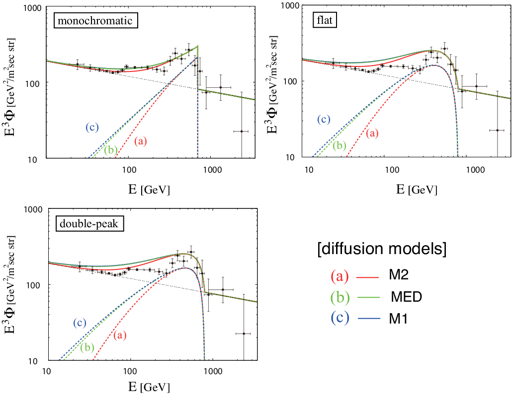
To see how the diffusion models affect the electron flux, we show in Fig. 4 the electron flux for the three diffusion models in the decaying dark matter scenarios with the three initial spectra. The parameters are the same as before. Note that those features in the electron fluxes are not sensitive to the diffusion models, especially in the high energy region (say $E\gtrsim(400-500)$ GeV). In the low energy region, the diffusion modes slightly affect the electron flux; the M1 and MED models predict a flatter spectrum than that in the M2 model. This opens up a possibility to sort out the dark matter models without suffering an uncertainty as to the diffusion processes in the galaxy, especially if we focus on the high-end of the electron flux ^#7^#7 #7 In this letter we do not take into consideration the electron spectrum below $400$ GeV, because there might be a possible contribution from the nearby pulsars [5], and because the diffusion-model dependence may not be negligible. .

Lastly, we show in Fig. 5 the electron spectra in both decaying and annihilating dark matter for the M2 and M1 diffusion models, where we have set the cross section and the mass as

\left\langle\sigma v\right\rangle\;=\;0.7\times 10^{-23}{\rm cm}^{3}/{\rm sec}{\rm~~and}~~m_{X}=700{\rm\,GeV}

(18)

for the monochromatic spectrum, and

\left\langle\sigma v\right\rangle\;=\;2.4\times 10^{-23}{\rm cm}^{3}/{\rm sec}{\rm~~and}~~m_{X}=800{\rm\,GeV}

(19)

for the flat and double-peak ones. The mass and lifetime for the decaying dark matter are same as before. As mentioned in the previous subsection, the electron spectra in the annihilating dark matter scenario look quite similar to those in the decaying one especially in the M2 model. Although not shown in the figure, the MED diffusion model is somewhat between the two models. Also one can more clearly see the difference between the flat and double-peak spectra in Fig. 5.

III Future experiments and dark matter model selection

In this section we roughly estimate how much statistics and precision are needed in future experiments in order to tell one dark matter model from another. Before proceeding further, however, it will be useful to briefly review the Fermi and CALET experiments.

In the near future, we expect to measure the energy spectrum of the cosmic-ray electrons more precisely. The Fermi satellite [17] has an $18$ silicon-strip tracker and an $8.5\,X_{0}$ thick CsI calorimeter ^#8^#8 #8 $X_{0}$ denotes the radiation length. with a geometric factor about $5\,{\rm\,m}^{2}{\rm\,str}$ and the energy resolution of about $5-10$ % over the energy range between $10$ and $300$ GeV. The central issue is how to select electrons while suppressing the hadron (mainly proton) contamination. After applying a set of selections [18], the residual proton contamination is found to be around $3$ % while retaining almost $30$ % of electrons, and the geometric factor for electrons turns out to be around $0.8{\rm\,m}^{2}{\rm str}$ ( $0.6{\rm\,m}^{2}{\rm str}$ ) at $600(800)$ GeV with an energy resolution of $5$ % at $20$ GeV to $20$ % at $1000$ GeV.

There is also a dedicated experiment proposed to measure the electron spectrum; CALET [19] is an instrument to observe very high energy electrons and gamma rays on JEM-EF of ISS. The CALET detector, developed based on the previous PPB-BETS balloon experiments, aims to measure the cosmic-ray electrons from $1$ GeV to $10$ TeV with an energy resolution better than a few % for energies greater than 100 GeV. The CALET detector consists of a combination of an imaging calorimeter IMC and a total absorption calorimeter TASC. (See Fig. 6) The geometric factor for electrons is $0.7{\rm\,m}^{2}$ str. The IMC can achieve the precision necessary to measure the starting point of an electro-magnetic shower and identify the incident particle. The TASC measures the development of electro-magnetic showers to determine the energy of the incident particle. One of the outstanding features of the CALET detector is that it achieves $32.8X_{0}$ (IMC $+$ TASC), which is large enough to get rid of the proton contamination efficiently even at an electron energy of $10$ TeV. The energy resolution is estimated to be $7{\rm\%}/(\sqrt{E/10{\rm GeV)}}$ [19]. The experiment was recently approved for a phase A study aiming at launching the detector in 2013 for a $5$ -year observation.

We have seen from Fig. 3 that the monochromatic initial spectrum results in the electron flux with a sharp drop-off. Let us study whether we can see such a feature in the energy spectrum when measured with the energy resolution of the Fermi and CALET experiments. The result is shown in Fig. 7, where we have set the dark matter mass $m_{X}=600(700)$ GeV for the monochromatic(flat) initial spectrum and the cross section $\left\langle\sigma v\right\rangle=0.8(2.4)\times 10^{-23}\,{\rm cm}^{3}/{\rm sec}$ . We have adopted the annihilating dark matter with the MED diffusion model, although the result is not sensitive to the decay/annihilation nor to the diffusion models (see Figs. 4 and 5). The dotted lines are the original ones corresponding to the monochromatic and flat initial spectra without smearing, while the solid (long-dashed) lines are obtained after taking account of the smearing effect based on the expected Fermi (CALET) energy resolution. Here we take $10$ % energy resolution for Fermi and $(7{\rm}/(\sqrt{E/10{\rm GeV}})\oplus 1)$ % for CALET, where $1\%$ stands for (unknown) systematic error. We can see that, even with the accuracy of the Fermi satellite, the sharp edge of the energy spectrum at $E=600$ GeV is smeared out, resulting in a smooth transition from $500$ GeV to $700$ GeV (solid), which is less prominent compared to that expected for CALET (long dashed). We expect that the accuracy of the Fermi satellite is good enough to measure the kinematic structure in the case of the monochromatic spectrum. In a case of the flat spectrum, however, the expected spectrum for Fermi is too broad to extract the dark matter mass, which may leave room for astrophysical interpretations.

Let us now investigate the electron energy distribution for the flat and double peak initial spectra. From Fig. 7 we expect that CALET can clearly measure the end point of the dark matter signal. In Fig. 8 we show the expected statistics at CALET for the annihilating dark matter scenario with the double-peak initial spectrum (iii), using the MED and M2 diffusion models. We have adopted the dark matter mass $m_{X}=800$ GeV, and the annihilation cross section $\left\langle\sigma v\right\rangle=2.4\times 10^{-23}{\rm cm}^{3}/{\rm sec}$ . Here we assume an exposure of $3\,\,{\rm m}^{2}\,{\rm str\,years}$ , and the errors take into account only the statistics. To avoid the uncertainty in the diffusion models, we focus on the flux in the high energy region, i.e., $E>500$ GeV. Indeed the MED and M2 diffusion models do not show any difference in the plotted region (the upper solid line corresponds to the MED model). From the plot, it is obvious that the sharp end of the distribution will exclude expected astrophysical sources.

We also show the distribution for the flat source spectrum for $m_{X}=800$ GeV (short dashed line). The distribution is normalized so that it is consistent to the double-peak spectrum at $500$ GeV by increasing the pair annihilation cross section. Although the distribution is quite similar to the solid line, we find more than $1\sigma$ difference over $11$ bins between $570$ GeV and $770$ GeV.

Note that the double-peak distribution is an unique signature that the parent particle is a vector. Although the propagation model we take in this paper is rather simple, it is tempting to estimate the $\chi^{2}$ difference between the two signal profiles quantitatively. For this purpose, let us define $\delta\chi^{2}$ as

\delta\chi^{2}\;=\;\sum_{i}\frac{(\phi_{T,i}-\phi_{{\rm flat},i})^{2}(\Delta E)^{2}\,\Omega^{2}}{\sigma_{i}^{2}},

(20)

where $\phi_{T,i}$ and $\phi_{{\rm flat},i}$ denote the electron flux for the double-peak and the flat source spectra, respectively, $\Delta E$ is the width of the energy bin, $\Omega$ is the exposure, $\sigma_{i}$ denotes the standard deviation, and the summation is taken over the energy bins from $500$ GeV to $900$ GeV. Here we take $\sigma_{i}^{2}=N_{i}$ , where $N_{i}$ is the number of events in an $i$ -th bin.

We have obtained $\delta\chi^{2}\simeq 74.6$ when calculated for $m_{X}=800$ GeV and the flux is normalized so that they are the same at $E=500$ GeV. If we minimize the $\delta\chi^{2}$ by varying $m_{X}$ with the distribution normalized at 500 GeV, we find the minimum value of $\delta\chi^{2}\simeq 31.8$ for $m_{X}=820$ GeV, corresponding to more than $5\sigma$ deviations.

IV Discussion and Conclusions

In this letter we have estimated the electron energy spectrum at the solar system for the three different initial energy spectra, $dN_{e}/dE$ , given by (1) - (5), in both decaying and annihilating dark matter scenarios, varying the diffusion model parameters. We have found that the difference in the initial spectra are reflected in the electron flux measured at the Earth even after long propagation through the galaxy. We have explicitly shown that such behavior is robust against changing diffusion parameters as long as we are concerned with the electron flux in the high energy region (say $E\gtrsim 400-500$ GeV). This observation will enable us to sort out dark matter models by precisely measuring the electron energy spectrum in a future observation such as CALET or the Fermi satellite in operation. We have also shown that the discontinuity predicted by the monochromatic initial spectrum (i) can be identified with an energy resolution of Fermi, while the other spectra (ii) and (iii) are less prominent as the electron spectrum from supernova remnant will also drop significantly with a certain energy cutoff. Also we have studied if we can distinguish the flat and double-peak initial spectra, which result in relatively similar energy spectra at the solar system. We have seen that the end point of the electron spectrum will be clearly seen with the resolution of about a few % assuming the statistics consistent with the ATIC anomaly, and that it will be possible to distinguish the two models at more than $5\sigma$ C.L. for the expected statistics at CALET.

Acknowledgements.

We would like to thank Satoshi Shirai and Tsutomu Yanagida for useful discussions. C.R.C. thanks Institute of Physics, Academia Sinica in Taiwan for its hospitality, where part of the work was done. This work was supported by World Premier International Research Center Initiative (WPI Initiative), MEXT, Japan.

References

[1] O. Adriani et al., arXiv:0810.4995 [astro-ph].
[2] J. Chang et al/, Nature 456 (2008) 362-365.
[3] S. Torii et al., arXiv:0809.0760 [astro-ph].
[4] F. A. Aharonian, A. M. Atoyan and H. J. Volk, Astron. Astrophys. 294, L41 (1995).
[5] D. Hooper, P. Blasi and P. D. Serpico, arXiv:0810.1527 [astro-ph];
H. Yuksel, M. D. Kistler and T. Stanev, arXiv:0810.2784 [astro-ph].
[6] S. Heinz and R. A. Sunyaev, Astron. Astrophys. 390, 751 (2002) [arXiv:astro-ph/0204183].
[7] C. R. Chen, F. Takahashi and T. T. Yanagida, arXiv:0809.0792 [hep-ph]; arXiv:0811.0477 [hep-ph]; A. E. Nelson and C. Spitzer, arXiv:0810.5167 [hep-ph]; I. Cholis, D. P. Finkbeiner, L. Goodenough and N. Weiner, arXiv:0810.5344 [astro-ph]; Y. Nomura and J. Thaler, arXiv:0810.5397 [hep-ph]; R. Harnik and G. D. Kribs, arXiv:0810.5557 [hep-ph]; D. Feldman, Z. Liu and P. Nath, arXiv:0810.5762 [hep-ph]; C. R. Chen and F. Takahashi, arXiv:0810.4110 [hep-ph]; P. f. Yin, Q. Yuan, J. Liu, J. Zhang, X. j. Bi and S. h. Zhu, arXiv:0811.0176 [hep-ph]; Y. Bai and Z. Han, arXiv:0811.0387 [hep-ph]; P. J. Fox and E. Poppitz, arXiv:0811.0399 [hep-ph]; K. Hamaguchi, E. Nakamura, S. Shirai and T. T. Yanagida, arXiv:0811.0737 [hep-ph]; T. Hur, H. S. Lee and C. Luhn, arXiv:0811.0812 [hep-ph]; E. Ponton and L. Randall, arXiv:0811.1029 [hep-ph]; M. Pospelov, arXiv:0811.1030 [hep-ph]; S. Baek and P. Ko, arXiv:0811.1646 [hep-ph]; E. J. Chun and J. C. Park, arXiv:0812.0308 [hep-ph]; M. Pospelov and M. Trott, arXiv:0812.0432 [hep-ph]; A. Arvanitaki, S. Dimopoulos, S. Dubovsky, P. W. Graham, R. Harnik and S. Rajendran, arXiv:0812.2075 [hep-ph]; R. Allahverdi, B. Dutta, K. Richardson-McDaniel and Y. Santoso, arXiv:0812.2196 [hep-ph]; K. Hamaguchi, S. Shirai and T. T. Yanagida, arXiv:0812.2374 [hep-ph].
[8] O. Adriani et al., arXiv:0810.4994 [astro-ph].
[9] A. Yamamoto et al., Adv. Space Res. 42, 442 (2008).
[10] C. R. Chen, F. Takahashi and T. T. Yanagida, in Ref. [7]; C. R. Chen, Mihoko M. Nojiri, F. Takahashi and T. T. Yanagida, arXiv:0811.3357 [astro-ph].
[11] T. Asaka, K. Ishiwata and T. Moroi, Phys. Rev. D 73, 051301 (2006) [arXiv:hep-ph/0512118].
[12] C. R. Chen and F. Takahashi, arXiv:0810.4110 [hep-ph].
[13] F. Takayama and M. Yamaguchi, Phys. Lett. B 485, 388 (2000) [arXiv:hep-ph/0005214].
[14] W. Buchmuller, L. Covi, K. Hamaguchi, A. Ibarra and T. Yanagida, JHEP 0703, 037 (2007) [arXiv:hep-ph/0702184].
[15] A. Ibarra and D. Tran, JCAP 0807, 002 (2008) [arXiv:0804.4596 [astro-ph]]; K. Ishiwata, S. Matsumoto and T. Moroi, arXiv:0805.1133 [hep-ph];
[16] I. Cholis, L. Goodenough and N. Weiner, arXiv:0802.2922 [astro-ph]; See also N. Arkani-Hamed, D. P. Finkbeiner, T. Slatyer and N. Weiner, in Ref. [7].
[17] Fermi Gamma-ray Space Telescope (formerly GLAST) collaboration, see the webpage: http://fermi.gsfc.nasa.gov/
[18] A. A. Moiseev, J. F. Ormes and I. V. Moskalenko, arXiv:0706.0882 [astro-ph].
[19] S. Torii [CALET Collaboration], Nucl. Phys. Proc. Suppl. 150, 345 (2006); J. Phys. Conf. Ser. 120, 062020 (2008).
[20] J. Hall and D. Hooper, arXiv:0811.3362 [astro-ph].
[21] V. Barger, W. Y. Keung, D. Marfatia and G. Shaughnessy, arXiv:0809.0162 [hep-ph].
[22] T. Delahaye, R. Lineros, F. Donato, N. Fornengo and P. Salati, Phys. Rev. D 77, 063527 (2008) [arXiv:0712.2312 [astro-ph]].
[23] L. Bergstrom, P. Ullio and J. H. Buckley, Astropart. Phys. 9, 137 (1998) [arXiv:astro-ph/9712318].
[24] J. Hisano, S. Matsumoto, O. Saito and M. Senami, Phys. Rev. D 73, 055004 (2006) [arXiv:hep-ph/0511118].