Inspired by the study of community structure in connection networks, we introduce the graph polynomial , the bivariate generating function which counts the number of connected components in induced subgraphs.
We give a recursive definition of using vertex deletion, vertex contraction and deletion of a vertex together with its neighborhood and prove a universality property. We relate to other known graph invariants and graph polynomials, among them partition functions, the Tutte polynomial, the independence and matching polynomials, and the universal edge elimination polynomial introduced by I. Averbouch, B. Godlin and J.A. Makowsky (2008).
We show that is vertex reconstructible in the sense of Kelly and Ulam, discuss its use in computing residual connectedness reliability. Finally we show that the computation of is -hard, but Fixed Parameter Tractable for graphs of bounded tree-width and clique-width.
1. Introduction
1.1. Motivation: Community Structure in Networks
In the last decade stochastic social networks have been analyzed mathematically from various points of view. Understanding such networks sheds light on many questions arising in biology, epidemology, sociology and large computer networks. Researchers have concentrated particularly on a few properties that seem to be common to many networks: the small-world property, power-law degree distributions, and network transitivity, For a broad view on the structure and dynamics of networks, see [36]. M. Girvan and M.E.J. Newman, [24], highlight another property that is found in many networks, the property of community structure, in which network nodes are joined together in tightly knit groups, between which there are only looser connections.
Motivated by [35], and the first author’s involvement in a project studying social networks, we were led to study the graph parameter , the number of vertex subsets with vertices such that has exactly components. , counts the number of degenerated communities which consist of members, and which split into isolated subcommunities.
The ordinary bivariate generating function associated with is the two-variable graph polynomial
We call the subgraph component polynomial of . The coefficient of in is the ordinary generating function for the number of vertex sets that induce a subgraph of with exactly components.
1.2. as a Graph Polynomial
There is an abundance of graph polynomials studied in the literature, and slowly there is a framework emerging, [30, 31, 25], which allows to compare graph polynomials with respect to their ability to distinguish graphs, to encode other graph polynomials or numeric graph invariants, and their computational complexity. In this paper we study the subgraph component polynomial as a graph polynomial in its own right and explore its properties within this emerging framework.
Like the bivariate Tutte polynomial, see [10, Chapter 10], the polynomial has several remarkable properties. However, its distinguishing power is quite different from the Tutte polynomial and other well studied polynomials.
Our main findings are:
- •
- •
Nevertheless, we construct an infinite family of pairs of graphs which cannot be pairwise distinguished by (Proposition 20).
- •
The Tutte polynomial, satisfies a linear recurrence relation with respect to edge deletion and edge contraction, and is universal in this respect. also satisfies a linear recurrence relation, but with respect to three kinds of vertex elimination, and is universal in this respect. (Theorems 13 and 21).
- •
A graph polynomial in three indeterminates, , which satisfies a linear recurrence relation with respect to three kinds of edge elimation, and which is universal in this respect, was introduced in [4, 5]. It subsumes both the Tutte polynomial and the matching polynomial. For a line graph of a graph , we have is a substitution instance of (Theorem 22).
- •
- •
- •
- •
Also like for the Tutte polynomial, cf. [27], has the Difficult Point Property, i.e. it is -hard to compute for all fixed values of where is a semi-algebraic set of lower dimension (Theorem 29). In [31] it is conjectured that the Difficult Point Property holds for a wide class of graph polynomials, the graph polynomials definable in Monadic Second Order Logic. The conjecture has been verified only for special cases, [6, 7, 8].
- •
Outline of the paper
The paper is organized as follows: In Section 2 we introduce the polynomial and its univariate versions. In Seection 3 we discuss the distinguishing power of and compare this to other graph polynomials. In Section 4 we show how certain graph parameters are definable using and relate it to partition functions and counting weighted homomorphisms. In Section 5 we give a recursive defintion of using deletion, contraction and extraction of vertices and show that is universal. We also compare it to the universal edge elimination polynomial defined in [4, 5] and give a subset expansion formula for . In Section 6 we prove decomposition formulas for for clique separators. In Section 7 we show the reconstructibility of . In Section 8 we discuss its use to compute the residual connectedness reliability. In Section 9 we discuss the complexity of computing . In Section 10 we draw conclusions and state open problems.
2. The Subgraph Component Polynomial
2.1. The Bivariate Polynomial
Let be a finite undirected graph with vertices and let be a positive integer. Assume the vertices of fail stochastic independently with a given probability . What is the probability that a subgraph of with exactly components survives? The solution of this problem leads to the enumeration of vertex induced subgraphs of with components. For a given vertex subset , let be the vertex induced subgraph of with vertex set and all edges of that have both end vertices in . We denote by the number of components of . Let be the number of vertex subsets with vertices such that has exactly components:
The ordinary generating function for these numbers is the two-variable polynomial
We call the subgraph component polynomial of . Since loops or parallel edges do not contribute to connectedness properties of a graph, we assume in this paper that all graphs are simple.

The star , presented in Figure 1, has the subgraph polynomial
The term tell us that there are 3 possibilities to select two vertices of that are non-adjacent.
The empty set induces the null graph that we consider as being connected, which gives for any graph. Substitution of for results in an univariate polynomial that is the ordinary generating function for all subsets of , i.e. .
2.2. Univariate Polynomials
The coefficient of in is the ordinary generating function for the number of vertex sets that induce a subgraph of with exactly components:
We call the polynomial for again subgraph component polynomial. The subscript as well as the number of variables should avoid confusion with the formerly defined subgraph polynomial. The subgraph polynomial is of special interest. We rename this polynomial to
It counts the connected vertex induced subgraphs of . A separating vertex set of a connected graph is a subset such that is a disconnected graph.
Theorem 1.
Let be a connected graph with vertices. Let be the number of separating vertex sets of cardinality for . Then the coefficients of the subgraph polynomial are given by
Proof.
If is a separating vertex set then induces a disconnected graph. Conversely, if is not a separating vertex set of then is connected. ∎
We conclude that is the number of all separating vertex sets of .

A graph invariant is on a class of graphs of for any two graphs and with the same number of vertices we have .
Proposition 2.
All non-isomorphic trees with up to nine vertices have different subgraph component polynomials. In other words we have: The graph polynomials and are not trivial on trees.
However, we have:
Proposition 3.
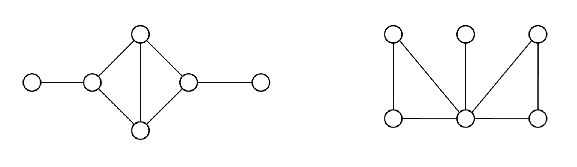
There exist a unique pair of non-isomorphic trees with vertices sharing the same subgraph component polynomial.
Proof.
Figure 2 shows these trees. This statement is true for as well as for the (general) subgraph polynomial . ∎
In Section 5 we shall see how to use this to generate infinite families of pairs of graphs which are not distinguished by .
3. Distinctive Power
We denote by be the matching polynomial with the number of -matchings of , by be the characteristic polynomial, by the Tutte polynomial, and by the bivariate chromatic polynomial introduced in [18].


Proposition 4.
Proof.
Remark 5.
does not distinguish between graphs which differ only by the multiplicity of their edges, whereas for the Tutte polynomial this is not the case. Let denote the complete graph with edges between any two distinct vertices. Then we have but .
Problem 6.
Are there simple graphs distinguished by , , or which are not distinguished by ?
We say that a simple graph is determined by a graph polynomial if for every simple graph such that we have that is isomorphic to . The class of simple graphs is determined by a graph polynomial if every graph is determined by . This notion has been studied in [38, 16], for the chromatic polynomial, the Tutte polynomial and the matching polynomial. It is shown, e.g., that several well-known families of graphs are determined by their Tutte polynomial, among them the class of wheels, squares of cycles, complete multipartite graphs, ladders, Möbius ladders, and hypercubes.
It follows from Proposition 8 that the class of empty graphs is determined by , and so is the class of complete graphs . Note that, since for all , the class of empty graphs is not determined by the the Tutte polynomial. It follows from Proposition 3 that the class of trees is not determined by .
Proposition 7.
The class of graphs of the form is determined by .
Proof.
It is easy to verify, that if , and , then is isomorphic to . ∎
4. Combinatorial Interpretations
4.1. Evaluations and Coefficients of
For a polynomial , let be the coefficient of in and let be the degree with respect to the variable .
Proposition 8.
The following graph properties can be easily obtained from the subgraph polynomial:
- (1)
The number of vertices:
- (2)
The number of edges:
- (3)
The number of components:
Theorem 9.
The degree of the subgraph component polynomial with respect to is the cardinality of a maximum independent set of (the independence number):
Proof.
Let be a maximum independent set of . In this case, we have and hence . Assume that there exists a set with . Then we obtain an independent set by selecting one vertex of each component of such that – a contradiction. ∎
Let be the number of independent vertex sets of size of . The independence polynomial of is defined by
As a consequence of Theorem 9 we can derive the independence polynomial of from the subgraph component polynomial. Let denote the coefficient of in . This coefficient is a polynomial in where the coefficient of counts the vertex subsets of cardinality of that induce a subgraph with components. A vertex set is independent if and only if . Hence is the number of independent vertex sets of size of .
4.2. Partition Functions
In this subsection we show that the subgraph polynomial for any and fixed can be viewed as a partition function, using counting of weighted graph homomorphisms. Partition functions were first studied in the context of statistical physics and have recently attracted much attention, [34]. A systematic study of the question which graph invariants can be presented as partition functions has been initiated in [23].
A weighted graph consists of a graph with assigning weights to vertices and to edges. The partition function associated with is defined by

Let be a weighted star with vertices and with all loops. The central vertex is . An example of for is shown on Figure 6. The weight functions are defined as follows:
Theorem 10.
Let be the partition function associated with and as above. Then, for all nonnegative integers and all , we have
Proof.
Let us start with the definition of . Under every mapping , let be the subset of vertices that are not mapped to . Let us count the homomorphisms that map the subset into : there are exactly such homomorphisms, because every connected component of must be mapped into a single vertex. Finally, we get
which by (10) completes the proof ∎
It is open whether there are other points in which is definable as a partition function.
Remark 11.
The auxiliary graph is called in physical literature The Widom-Rowlinson model for particles. The homomorphisms to are called Widom-Rowlinson configurations, [20].
5. Recursive Definition and Subset Expansion
5.1. Recurrence Relation for Vertex Elimination
We turn now our attention to the investigation of properties of the subgraph polynomial that support its computation. The first statement concerns the multiplicativity with respect to components of the graph.
Theorem 12 (Multiplicativity).
- (1)
Let be the disjoint union of the graphs and . Then
- (2)
In particular, if consists of components then the subgraph polynomial satisfies
Proof.
In case , each subset of cardinality is the disjoint union of two subsets and with and . The number of components of is the sum of the number of components of and . We obtain
| (3) |
Thus for a graph with two components, the subgraph polynomial satisfies
We obtain the statement of the theorem by induction on the number of components. ∎

We distinguish three types of vertex elimination:
- Vertex deletion:
-
For a given vertex , let the graph obtained from by removal of and all edges that are incident to . We call this operation vertex deletion.
- Vertex extraction:
-
Similarly, let be the graph obtained from by removal of all vertices of the set . Let be the set of vertices that are adjacent to in (the neighborhood of ). We denote by the closed neighborhood of a vertex in , i.e. the set of all vertices adjacent to including itself. The operation is called vertex extraction.
- Vertex contraction:
-
A further special graph operation is needed here – the contraction of a vertex. That is the graph obtained from by removal of and insertion of edges between all pairs of non-adjacent neighbor vertices of . Figure 7 shows an example graph and the graph obtained by vertex contraction.
Theorem 13.
Let be a graph and . Then the subgraph polynomial satisfies the decomposition formula
Proof.
Let us first consider all vertex induced subgraphs of that do not contain vertex . These subgraphs are also vertex induced subgraphs of . Consequently,
enumerates all induced subgraphs not including the vertex .
In a second step we count all vertex induced subgraphs that contain vertex but none of its neighbors in . In this case, the vertex forms a connected component consisting of only. The rest of the induced subgraph is a subgraph of of . All these subgraphs are enumerated by . However, the component built by contributes one vertex and one component to the polynomial. Thus we obtain the generating function
In our enumeration so far we missed exactly those vertex induced subgraphs that contain and at least one of its neighbors together in one component. We include in the corresponding candidate set, remove it from , and multiply the generating function by (not by because we do not increase the number of components). In order to trace the components, we have to simulate the paths using in . These paths are no longer present in . This task is best performed by using instead of . Thus we obtain the contribution to the generating function. Unfortunately, this polynomial enumerates induced subgraphs that do not contain any vertices from , too. We can fix this problem by subtraction of , which gives
as final contribution to the generating function. ∎
Corollary 14.
Let be a vertex of degree 1 in and let be its only neighbor in . Then
Proof.
Notice that in this case and . Then the statement follows immediately from Theorem 13. ∎
5.2. Some Easy Computations
The subgraph polynomial can be easily computed for certain special graphs.
Proposition 15.
For the complete graphs and the empty graphs (the complement of ) we have:
- (1)
.
- (2)
.
Proof.
(1) In a complete graph each vertex subset except the empty set induces a connected subgraph.
(2) In the empty graph each subset induces a subgraph with components. ∎
From Theorem 13 we obtain a recurrence relation for the subgraph polynomial of the paths :
Proposition 16.
Together with the initial values,
equation (16) determines the subgraph polynomial of uniquely. The explicit solution is
with .
The subgraph polynomial of the cycle satisfies another recurrence relation:
Proposition 17.
The join of two graphs and with is the graph obtained from by introducing edges form each vertex of to each vertex of . Consequently, the join of two empty graphs and is the complete bipartite graph .
Theorem 18.
Let and be two graphs with , , . Then
Proof.
All vertex subsets of belong to exactly one of three classes:
(1) subsets of ,
(2) subsets of
(3) subsets that have at least one vertex of and at least one vertex of
.
The first two classes are counted by and , respectively. The empty set is counted twice, which is corrected by subtracting one. All vertex subsets of the third class induce connected subgraphs of . The generating function for the number of subsets of this class is . ∎
From Theorem 18, we deduce the subgraph polynomial of the complete bipartite graph:
Corollary 19.
Propositions 16 and 17 and Theorem 18 are explicit instances of general results which follow from the fact that is definable in Monadic Second Order Logic. We shall discuss this feature in Section 5.5.
We can use Theorem 18 and the multiplicativity of to prove the following:
Proposition 20.
There are infinite families of pairs of non-isomorphic graphs with a fixed number of connected components which are not distinguished by .
5.3. The Universality Property of
The vertex decomposition formula represented in Theorem 13 can be considered as a vertex equivalent to the well-known edge decomposition (deletion-contraction relations). Edge decomposition formulae of the form apply to the Tutte polynomial and derived graph invariants, for instance the number of spanning trees or the reliability polynomial. Indeed, it was shown by J.G. Oxley and D.J.A. Welsh, [41], that the Tutte polynomial is in a certain sense universal, meaning that all other graph invariants that satisfy edge decomposition formulae can be derived from the Tutte polynomial by substitution of variables. A textbook presentation is given in [10]. A general framework analyzing universality properties of graph polynomials is studied in [25].
It seems natural to ask for the most general vertex decomposition formula. Let us assume that we try to construct an ordinary generating function that counts some type of vertex induced subgraphs with respect to the number of vertices. Which properties should such a function have? If the subgraphs in question are composed from subgraphs of the components then we can expect multiplicativity of with respect to components of the graph. In order to assign the value uniquely to a graph by application of a decomposition formula as given in Theorem 13, certain initial values for the null graph and the empty graph have to be given. Therefore, we presuppose the following four properties of :
- (a)
(Multiplicativity) If and are components of then .
- (b)
(Recurrence relation) Let and let be a vertex of , then
(4) - (c)
(Initial condition) There exists such that for the null graph .
- (d)
(Initial condition) There exists such that for a graph consisting of one vertex.
Furthermore, in order to make a well-defined graph polynomial, the result of computing has to be the same, irrespective of the order in which we apply the enabled computation steps. In particular, it has to be independent of the order of the vertices, which we use to apply the decomposition formula (b). In general we may choose from a field of characteristic zero or from a ring. A graph invariant is proper if there are two graphs and with the same number of vertices such that .
Applying the conditions (b), (c), and (d) we obtain from the equation
Computing in two ways using (a) and (b), respectively, results in
Consequently, the values of and are determined:
If the constants are properly defined then the value of does not depend on the choice of the vertex in equation (4). Consequently, the function does not depend on the order of the vertex decomposition (4). The calculation of for path of three vertices yields, in case we start from a vertex of degree 1,
If we begin the vertex decomposition at the vertex of degree 2 then we obtain
These two results coincide if , , or . In any case, there remain only two variables that can be chosen independently. In case of , all graphs with the same number of vertices result in the same polynomial. Therefore, this case does not yield any interesting applications. If then for all graphs. The only remaining choice, , gives for and the subgraph component polynomial .
From this we get that is universal among polynomials recursively defined using vertex deletion, vertex extraction and vertex contraction. More precisely, we have the following theorem.
Theorem 21 (Universality of ).
- (1)
For a graph polynomial to be proper and well-defined by conditions (a)-(d) we have , and .
- (2)
There is a unique proper graph polynomial which is well-defined by conditions (a)-(d) and we have
and
5.4. Vertex Eliminations vs Edge Elimination
The subgraph component polynomial can be regarded as counting vertex set expansions. In the literature there is a variety of graph polynomials, including the Tutte polynomial, which can be defined by counting edge set expansions.
We have seen in Theorem 21 that is universal among the polynomials defined recursively via deletion, extraction and contraction of vertices. In [4, 5] the polynomial was shown to be universal among the polynomials defined recursively via deletion, extraction and contraction of edges. In this section we will show the connection of to the universal edge elimination polynomial .
The polynomial generalizes both the Tutte and the matching polynomials, as well as the bivariate chromatic polynomial of [18]. We shall use the recursive decomposition of from [5]:
| (5) |
where denotes the disjoint union of graphs and , and the three edge elimination operations are defined as follows:
- Edge deletion::
-
We denote by the graph obtained from by simply removing the edge .
- Edge extraction::
-
We denote by the graph induced by provided . Note that this operation removes also all the edges adjacent to .
- Edge contraction::
-
We denote by the graph obtained from by unifying the endpoints of .
We will rewrite the decomposition of using Theorem 13.
| (6) |
Theorem 22.
Let be a graph. Let denote the line graph of . Then the following equation holds:
Proof.
First, let us analyze the correspondence of the edge elimination operations in a graph to the vertex elimination operations in its line graph. Let be the vertex in the line graph that corresponds to the edge of the original graph. By the definition of the edge and vertex elimination operations:
| (7) | |||
| (8) | |||
| (9) |
First let us check the connected graphs with up to one edge:
If , ,
The equivalence holds.
If is a single point with a loop, or , is a singleton, The equivalence holds.
Problem 23.
How does the distinguishing power of compare to the distinguishing power of ?
5.5. Subset Expansion and Definability in Logic
was defined as a generating function. Let us rewrite the definition of in a slightly different way. Instead of summation over the number of the used vertices , and the number of induced connected components , we shall summate over all the possible subsets of vertices:
| (10) |
This is a subset expansion formula, a term coined in [42]. The relationship between recursive definitions of graph polynomials and the existence of subset expansion formulas has been studied from a logical point of view in [25]. Subset expansion formulas can often be used to show that a graph polynomial is definable in Monadic Second Order Logic, as studied in [28, 31] . However, the exponent in Equation (10) causes a problem. to remedy this, we use, like in [29], an auxiliary order over the vertices. We will denote by the subset of the smallest vertices in every respective connected component.
| (11) |
Note that the result does not depend on the used auxiliary order.
Without having to go in the details of graph polynomials definable in Monadic Second Order Logic11 1 The interested reader can consult [21] for the use Monadic Second Order Logic in finite model theory, and [13] for its use in graph theory. , Equation (11) shows that is a graph polynomial definable in Monadic Second Order Logic for graphs with universe and a binary edge relation. Therefore all the theorems from [28, 32] can be applied. In particular, the Feferman-Vaught-type theorems from [28] guarantee existence of reduction formulas like multiplicativity from Theorem 12, or the one in Theorem 18 for the join, not only for the disjoint union or the join operation, but for a wide class of -definable operations. Also, a general theorem from [32] guarantees the existence of recurrence formulas, as proven in Propositions 16 and 17, for a wide class of recursively defined families of graphs, as studied also in [39]. Among these we have the wheels , the ladders and the stars . It should not be difficult to compute the recurrence relations for these explicitly.
We shall exploit -definability also for our complexity analysis in Section 9.2.
6. Clique Separators
The simplest case of a clique separator in a graph is an articulation, i.e. a vertex whose removal from results in an increase of the number of components. Let be an articulation of and let and be subgraphs of such that and . It is well known, cf. [10], that in this case the Tutte polynomial satisfies
In the case of the subgraph component polynomial the situation is a bit more complicated:
Theorem 24.
Let be an articulation of and let and be subgraphs of such that and . Then the subgraph polynomial satisfies
Proof.
The first product of the polynomial is the generating function for the number all vertex induced subgraphs that do not contain the articulation . The product is justified by Theorem 12. The second term counts all remaining subgraphs, i.e. those ones containing vertex . Here the equation (3) from the proof of Theorem 12 has to be modified. The vertex is counted twice because it belongs to both and . This double counting is corrected by multiplication with . By analogy, we introduce the factor in order to avoid that the component containing is counted twice. ∎
Theorem 24 can be generalized in order to cover clique separators with more than one vertex. Let be a connected graph and , subgraphs of such that and . In this case forms a separating clique of . Here we assume that neither nor coincides with . The subgraphs and are called split components of with respect to .
Theorem 25.
Let be a clique separator of such that there are two split components and . Then the subgraph polynomial satisfies
Proof.
First we count all subgraphs that are induced by vertex subsets included in . These subgraphs are also subgraphs of . From Theorem 12 we obtain as generating function for all subgraphs of induced by subsets of .
For each subset , let be the number of vertex subsets of cardinality with such that the induced subgraph has exactly components:
The polynomial
is the ordinary generating function for the numbers . We define the numbers and the corresponding generating function for the second split component analogously. Let be a vertex subset with . Then the component of that contains is counted in and in . There is indeed only one component counted twice, since induces a clique of and , respectively. Thus we obtain
| (12) |
The factor takes into account that all vertices of contribute to and to . For each subset , the subgraph polynomial of can be represented as a sum of generating functions as follows:
We define and obtain
or
By Möbius inversion, we obtain
Similarly, we can prove for each that
The substitution of and in equation (12) yields
∎
Problem 26.
Can we have an analogue of Theorem 25 for the case where the separating vertex set is not required to be a clique?
7. Reconstruction
The famous graph reconstruction conjecture by Kelly and Ulam [44] states the every undirected graph with at least three vertices can be reconstructed from a deck of its vertex-deleted subgraphs (more precisely from the corresponding isomorphism classes). See for example the papers [12, 11] as an introduction into this field. Despite the fact that the conjecture is still open, many graph invariants and graph polynomials (e.g. the Tutte polynomial) are known to be reconstructible. We can show that also the subgraph component polynomial can be reconstructed from the deck of the subgraph polynomials of the vertex-deleted subgraphs.
Theorem 27.
The subgraph polynomial for a graph with is uniquely determined by the set of polynomials
Let be the smallest power of that appears at least twice among the terms of the polynomials . Define
Then the subgraph polynomial is given by
Proof.
Let denote the number of components of a graph . In each graph with at least three vertices and at least one edge there exist two vertices such that . If the term appears in the polynomial then the number of components of equals . Since for each vertex , the the smallest power of that appears at least twice among the terms of the polynomials is equal to . There is only one exception: If is the empty (edgeless) graph then the removal of each vertex of decreases the number of components by one, which is taken into consideration within the definition of . Consequently, we obtain .
Each vertex induced subgraph with vertices is counted exactly times in the polynomial
The coefficient of in
equals times the number of vertex induced subgraphs of with exactly vertices and components. The integration with respect to transforms into such that the vertex induced subgraphs are enumerated correctly by the coefficients of the resulting polynomial. Finally, the bounds of integration and the multiplication with performs the back-substitution in order to obtain an ordinary generating function with variables and . ∎
8. Random Subgraphs
Now we assume that the vertices of fail stochastic independently with a given (identical) probability . We obtain the probability that a vertex induced subgraph of has exactly components from the subgraph polynomial:
| (13) |
The sequence is the distribution of the number of components. Consequently, we obtain


The probability is called the residual connectedness reliability. Boesch, Satyanarayana, and Suffel [9] showed that the computation of is a #P-hard problem, even in planar bipartite graphs. Since can be obtained in polynomial time from the subgraph polynomial by applying the relation (13), we obtain the following statement.
Corollary 28.
The computation of the subgraph polynomial is a #P-hard problem. It remains #P-hard for the class of all planar bipartite graphs.
9. Computational complexity of
9.1. Complexity of evaluation
We have already seen in Corollary 28 that is -hard to compute. Now we deal with a problem of evaluation of at a given point for arbitrary input graph .
Theorem 29.
For every point , possibly except for the lines , , and , the evaluation of for an input graph is -hard.
C. Hoffmann in [26] showed the following:
Theorem 30 (Hoffmann 2008).
For every point , except possibly for the subsets , , and , the evaluation of for an input graph is -hard.
Proof of Theorem 29:
The evaluation of is polynomial time computable for and for . It remains open whether it is polynomial time computable for and . One can also ask, whether there is some point , in which is hard to evaluate for general input graph, but easy for input line graph.
9.2. Parameterized complexity
Here we discuss the computational complexity of for input graphs of bounded tree with, and for input graphs for bounded clique width. We do not need the exact definitions here. For background on tree-width the reader can consult [17]. Clique-width was defined in [15]. Both are discussed in [28].
Recall that the subgraph component polynomial is definable using the -formalism (definition 11) with auxiliary order, while the result is order-independent. Hense, using a general theorem from [29, 28], we have
Proposition 31.
is polynomial time computable on graphs of tree-width at most where the exponent of the run time is independent of .
Moreover, applying the result of Courcelle, Makowsky and Rotics [14], combined with the results from [40], we have a similar result for graphs of bouded clique width:
Proposition 32.
is polynomial time computable on graphs of clique-width at most where the exponent of the run time is independent of .
The drawback of the general methods of [29, 28] and [14], lies in the huge hidden constants, which make it practically unusable. However, an explicit dynamic algorithm for computing the polynomial on graphs of bounded tree-width, given the tree decomposition of the graph, where the constants are simply exponential in , can be constructed along the same ideas as presented in [43, 22]. For the graphs of bounded clique width, given the clique decomposition of the graph, we know an algorithm with constants doubly-exponential in . It is open whether an algorithm with constants simply exponential in exists. For a comparison of the complexity of computing graph polynomials on graphs classes of bounded clique-width, cf. [33].
10. Conclusions and Open Problems
We have shown that is a universal vertex elimination polynomial. We have given a few combinatorial interpretations of its evaluations and coefficients. We have proven various splitting formulas for such as the multiplicativity, Theorem 13 and Theorem 25. Problem 26 asks for more such theorems. Besides having algorithmic importance, such splitting formulas increase our structural understanding of the graph polynomial under study, and may help us in analizing its distictive power.
We have looked at the graph polynomial from various angles and compared its behaviour and distinguishing power with the characteristic polynomial, the matching polynomial the Tutte polynomial and the universal edge elimination polynomial. We have not discussed the relationship of to other graph polynomials, such as the interlace polynomial, [3, 1], or the many other graph polynomials listed in [31].
We have seen that distinguishes between graphs where these polynomials do not. We have not found cases where these other polynomials do distinguish between graphs where does not. This is probably due to our lack of computerized tools for searching for such cases, cf. Problem 6. In Problem 23 we ask about comparing distinguishing power of and the universal edge elimination polynomial . This seems to be more tricky. We have given a few examples of graphs and graph families which are determined by .
Problem 33.
Find more graph invariants which are determined by .
Problem 34.
Find more classes of graphs which are determined by .
Returning to our motivation, we have only studied the simplest case of community structure in networks. We have studied the generating function of induced subgraphs with vertices which have components. More generally, one would want to study community structures where components are replaced by maximal -connected components.
Problem 35.
What are the appropriate generating functions which capture the essence of various community structures?
References
- [1] M. Aigner and H. van der Holst. Interlace polynomials. Linear Algebra and Applications, 377:11–30, 2004.
- [2] A. Andrzejak. Splitting formulas for Tutte polynomials. Journal of Combinatorial Theory, Series B, 70.2:346–366, 1997.
- [3] R. Arratia, B. Bollobás, and G.B. Sorkin. The interlace polynomial of a graph. Journal of Combinatorial Theory, Series B, 92:199–233, 2004.
- [4] I. Averbouch, B. Godlin, and J.A. Makowsky. The most general edge elimination polynomial. arXiv http://uk.arxiv.org/pdf/0712.3112.pdf, 2007.
- [5] I. Averbouch, B. Godlin, and J.A. Makowsky. An extension of the bivariate chromatic polynomial. submitted, 2008.
- [6] M. Bläser and H. Dell. Complexity of the cover polynomial. In L. Arge, C. Cachin, T. Jurdziński, and A. Tarlecki, editors, Automata, Languages and Programming, ICALP 2007, volume 4596 of Lecture Notes in Computer Science, pages 801–812. Springer, 2007.
- [7] M. Bläser and H. Dell. Complexity of the Bollobás-Riordan polynomia. exceptional points and uniform reductions. In Edward A. Hirsch, Alexander A. Razborov, Alexei Semenov, and Anatol Slissenko, editors, Computer Science–Theory and Applications, Third International Computer Science Symposium in Russia, volume 5010 of Lecture Notes in Computer Science, pages 86–98. Springer, 2008.
- [8] Markus Bläser and Christian Hoffmann. On the complexity of the interlace polynomial. In STACS, pages 97–108, 2008.
- [9] F. Boesch, A. Satyanarayana, and C. Suffel. On residual connectedness reliability. In F. Roberts, F. Hwang, and C. Monma, editors, Reliability of Computer and Communication Networks, volume 5 of DIMACS Series in Discrete Math. and Theor. Comp. Science, pages 51–59. AMS and ACM, 1991.
- [10] B. Bollobás. Modern Graph Theory. Springer, 1999.
- [11] J. A. Bondy. A graph reconstructor’s manual. In A.D. Keedwell, editor, Surveys in Combinatorics, 1991, volume 166 of London Mathematical Society Lecture Note Series, pages 221–252. Cambridge University Press, 1991.
- [12] J. A. Bondy and R.L. Hemminger. Graph reconstruction: A survey. Journal of Graph Theory, 1:227–268, 1977.
- [13] B. Courcelle. Graph Structure and Monadic Second Order Logic. Cambridge University Press, in preparation.
- [14] B. Courcelle, J.A. Makowsky, and U. Rotics. On the fixed parameter complexity of graph enumeration problems definable in monadic second order logic. Discrete Applied Mathematics, 108(1-2):23–52, 2001.
- [15] B. Courcelle and S. Olariu. Upper bounds to the clique–width of graphs. Discrete Applied Mathematics, 101:77–114, 2000.
- [16] A. de Mier and M. Noy. On graphs determined by their Tutte polynomials. Graphs and Combinatorics, 20.1:105–119, 2004.
- [17] R. Diestel. Graph Decompositions, A Study in Infinite Graph Theory. Clarendon Press, Oxford, 1990.
- [18] K. Dohmen, A. Pönitz, and P. Tittmann. A new two-variable generalization of the chromatic polynomial. Discrete Mathematics and Theoretical Computer Science, 6:69–90, 2003.
- [19] R.G. Downey and M.F Fellows. Parametrized Complexity. Springer, 1999.
- [20] M. Dyer and C. Greenhill. The complexity of counting graph homomorphisms. Random Structures and Algorithms, 17.3-4:260 – 289, 2000.
- [21] H. Ebbinghaus and J. Flum. Finite Model Theory. Springer Verlag, 1995.
- [22] E. Fischer, J.A. Makowsky, and E.V. Ravve. Counting truth assignments of formulas of bounded tree width and clique-width. Discrete Applied Mathematics, 156:511–529, 2008.
- [23] M. Freedman, László Lovász, and A. Schrijver. Reflection positivity, rank connectivity, and homomorphisms of graphs. Journal of AMS, 20:37–51, 2007.
- [24] M. Girvan and M.E.J. Newman. Community structure in social and biological networks. Proc. Natl. Acad. Sci. USA, 99:7821–7826, 2002.
- [25] B. Godlin, E. Katz, and J.A. Makowsky. Graph polynomials: From recursive definitions to subset expansion formulas. arXiv http://uk.arxiv.org/pdf/0812.1364.pdf, 2008.
- [26] C. Hoffmann. A most general edge elimination polynomial–thickening of edges. arXiv:0801.1600v1 [math.CO], 2008.
- [27] F. Jaeger, D.L. Vertigan, and D.J.A. Welsh. On the computational complexity of the Jones and Tutte polynomials. Math. Proc. Camb. Phil. Soc., 108:35–53, 1990.
- [28] J.A. Makowsky. Algorithmic uses of the Feferman-Vaught theorem. Annals of Pure and Applied Logic, 126.1-3:159–213, 2004.
- [29] J.A. Makowsky. Colored Tutte polynomials and Kauffman brackets on graphs of bounded tree width. Disc. Appl. Math., 145(2):276–290, 2005.
- [30] J.A. Makowsky. From a zoo to a zoology: Descriptive complexity for graph polynomials. In A. Beckmann, U. Berger, B. Löwe, and J.V. Tucker, editors, Logical Approaches to Computational Barriers, Second Conference on Computability in Europe, CiE 2006, Swansea, UK, July 2006, volume 3988 of Lecture Notes in Computer Science, pages 330–341. Springer, 2006.
- [31] J.A. Makowsky. From a zoo to a zoology: Towards a general theory of graph polynomials. Theory of Computing Systems, 43:542–562, 2008.
- [32] J.A. Makowsky and E. Fischer. Linear recurrence relations for graph polynomials. In A. Avron, N. Dershowitz, and A. Rabinowitz, editors, Boris (Boaz) A. Trakhtenbrot on the occasion of his 85th birthday, volume 4800 of LNCS, pages 266–279. Springer, 2008.
- [33] J.A. Makowsky, U. Rotics, I. Averbouch, and B. Godlin. Computing graph polynomials on graphs of bounded clique-width. In F. V. Fomin, editor, Graph-Theoretic Concepts in Computer Science, 32nd International Workshop, WG 2006, Bergen, Norway, June 22-23, 2006, Revised Papers, volume 4271 of Lecture Notes in Computer Science, pages 191–204. Springer, 2006.
- [34] J. Nesetril and P. Winkler, editors. Graphs, Morphisms and Statistical Physics, volume 63 of DIMACS Series in Discrete Mathematics and Theoretical Computer Science. AMS, 2004.
- [35] M.E.J. Newman. Detecting community structure in networks. Eur. Phys. J.B., 38:321–330, 2004.
- [36] M.E.J. Newman, A.L. Barabasi, and D. Watts. The Structure and Dynamics of Networks. Princeton University Press, 2006.
- [37] S.D. Noble. Evaluating the Tutte polynomial for graphs of bounded tree-width. Combinatorics, Probability and Computing, 7:307–321, 1998.
- [38] M. Noy. On graphs determined by polynomial invariants. tcs, 307:365–384, 2003.
- [39] M. Noy and A. Ribó. Recursively constructible families of graphs. Advances in Applied Mathematics, 32:350–363, 2004.
- [40] S. Oum. Approximating rank-width and clique-width quickly. In Graph Theoretic Concepts in Computer Science, WG 2005, volume 3787 of Lecture Notes in Computer Science, pages 49–58, 2005.
- [41] J.G. Oxley and D.J.A. Welsh. The Tutte polynomial and percolation. In J.A. Bundy and U.S.R. Murty, editors, Graph Theory and Related Topics, pages 329–339. Academic Press, London, 1979.
- [42] L. Traldi. A subset expansion of the coloured Tutte polynomial. Combinatorics, Probability and Computing, 13:269–275, 2004.
- [43] L. Traldi. On the colored Tutte polynomial of a graph of bounded tree-width. Discrete Applied Mathematics, 154.6:1032–1036, 2006.
- [44] S.M. Ulam. A Collection of Mathematical Problems. Wiley, 1960.