Relativistic orbits with gravitomagnetic corrections

The analogy between the classical Newton and Coulomb laws led to investigate if masses in motion, considered as charges, could give rise to a "gravitational" magnetic field.

In fact, the magnetic field is produced by the motion of electric-charge, i.e. the electric current. The analogy consists of the fact that a mass-energy current can produce what is called "gravitomagnetic" field.

The pioneering approach to the problem is due to Maxwell himself which, in one of his fundamental works on electromagnetism, turned his attention on the possibility to formulate the theory of gravitation in a form corresponding to the electromagnetic equations [1]. However, he was puzzled by the problem of the energy of the gravitational field, i.e. the meaning and the origin of the negative energy due to the mutual attraction of material bodies. In fact, according to him, the energy of a given field had to be "essentially positive", but this is not the case for the gravitational field. To balance this negative energy, a great amount of positive energy is required, in the form of energy of the space (a sort of back-reaction). But, since he was unable to understand how this could be, he did not proceed further along this line of thinking since the problem can be addressed and solved only in the framework of General Relativity.

Later, Holzmuller [2] and Tisserand [3] proposed to modify the Newton law introducing, in the radial component of the force, a term depending on the relative velocity of the two attracting particles (see also [4, 5]). Also Heaviside [6, 7] investigated the analogy between gravitation and electromagnetism considering the propagation of gravitational energy in terms of a sort of gravito - electromagnetic Poynting vector: however, also in this case, he failed to frame the problem of gravitational energy in a self-consistent scheme.

Finally, the formal analogy between electromagnetic and gravitational fields was explored by Einstein [8], in the framework of General Relativity, and then by Thirring [9]. This author pointed out that the geodesic equation can be written as a Lorentz force splitting the gravitational field in gravito-electric and gravito-magnetic components. The final result of these studies was that any theory which combines Newtonian gravity together with Lorentz invariance in a consistent way, has to include a gravitomagnetic field, which is generated by the mass-energy current. This is the case, of course, of General Relativity: it was shown by Lense and Thirring [10], that a rotating mass generates a gravitomagnetic field, which in turn, causes the precession of planetary orbits. To be more precise, H. Pfister has recently shown that it would be better to speak about an Einstein - Lense - Thirring effect [11].

It is interesting to notice that also Lodge and Larmor, at the end of the nineteenth century, discussed the effects of frame dragging on a non-rotating interferometer [12], but within the framework of an aether-theoretical model. This frame dragging corresponded, in fact, to the Lense-Thirring effect of General Relativity. However, at the beginning of the XX century, when Lense and Thirring published their papers, the effect named after them, which is indeed very small in the terrestrial environment, was far from being detectable, because of the technical difficulties and limitations of the time. Contemporary improvements in technology have made possible to propose new ideas to reveal the Lense-Thirring precession by analyzing the data-sets on the orbits of Earth satellites (see e.g. [13] where, for the first time, the use of LAGEOS satellite was proposed). Several proposals have been recently published to measure the Lense-Thirring effect by natural and artificial bodies in some Solar System scenarios. For example, in [14], the Sun with Venus is considered. Mars with MGS spacecraft is discussed in [15], while Jupiter with the Galilean moons (which is the original idea by Lense and Thirring) is studied in [16]. Regarding the Earth with the existing LAGEOS and LAGEOSII satellites, recent results are reported in [17], while for the approved experiment LARES the expected forthcoming measurement are discussed in [18].

On the other hand, the experiment Gravity Probe-B [19] has been devoted to another gravitomagnetic effect due to Earth’s rotation, i.e. the Pugh-Schiff effect consisting of the precessions of the spins of four gyroscopes carried onboard the spcaecraft [20, 21]. This experiment has detected the effect and its magnitude in the gravitational field of the Earth [22]. The originally expected accuracy was $1\%$ or better, but it is still unclear if it will be finally obtained because of unexpected systematic effects arisen in the data analysis. Other experiments (like GP-C [23, 24, 25]) have been proposed to reveal the space-time structure, which is affected by gravitomagnetism, for example evidencing clock effects around a spinning massive object. In particular, concerning the so-called gravitomagnetic clock effect, we have to stress that its most investigated form consists of the difference between the orbital periods of two counter-rotating satellites.

Recently, gravitomagnetic effects have been considered also in the framework of gravitational lensing. By using the Fermat principle and the standard theory of gravitational lensing, the gravitomagnetic corrections to the time delay function and the deflection angle for a geometrically thin lens can be derived. Such corrections can induce observational effects both in point-like [26] and in extended gravitational lenses (as the isothermal sphere and the disk of spiral galaxies [27, 28]. Other researches concerning the gravitomagnetic effects on time delay and light deflection have been pursued. In [29], the gravitomagnetic effects in the propagation of electromagnetic waves in variable gravitational fields of arbitrary-moving and spinning bodies have been studied, while, in [30, 31, 32], the gravitational lensing due to stars with angular momentum, and then inducing gravitomagnetic effects, have been considered.

Finally, the analogy between general relativity and electromagnetism suggests that there is also a galvano-gravitomagnetic effect, which is the gravitational analog of the Hall effect. This effect takes place when a current carrying conductor is placed in a gravitomagnetic field and the conduction electrons moving inside the conductor are deflected transversally with respect to the current flow. Such a galvano-gravitomagnetic effect, considering current carrying conductors, could be used for detecting the gravitomagnetic field of the Earth. A discussion of the effect and its measurability is in [33, 34, 35].

In this paper, we want to study how the relativistic theory of orbits for massive point-like objects is affected by gravitomagnetic corrections. In other words, we want to consider the orbital effects of higher-order terms in $v/c$ and this is the main difference with respect to the standard gravitomagnetic effect so far considered. In this case, the problem of gravitomagnetic vector potential entering into the off-diagonal components $g_{0l}$ of the metric $g_{\mu\nu}$ can be greatly simplified and the corrections can be seen as further powers in the expansion in $c^{-1}$ (up to $c^{-3}$). Nevertheless, the effects on the orbit behavior are interesting and involve not only the precession at peri-astron but also nutation corrections as we will show below. This means that it could be misleading to neglect such effects when the weak field approximation is not so weak, as in the case of point-like compact objects moving in a tight-binding regime or spiralizing each other as in the case of evolved binary systems constituted by black holes and/or neutron stars. A study in this sense is in [36] where the possibility of measuring the Lense-Thirring effect with the double pulsar J0737-3039A is discussed.

In particular, we can study the evolution of compact binary systems in the extreme mass ratio limit, i.e. the mass of the moving particle is $m$ and the mass that produces the gravitational field is $M$, so that $m\ll M$. This constraint is satisfied by several real systems. For example, there has been gathering evidence suggesting the existence of supermassive black hole with masses in the ranges $10^{6}\div 10^{9}M_{\odot}$) in galactic nuclei [37, 38]. One expects that small compact objects ($1\div 10M_{\odot}$) from the surrounding stellar population will be captured by these black holes following many-body scattering interactions at a relatively high rate [39, 40].

Our approach suggests that, in the weak field approximation, when considering higher order corrections in the motion equations, the gravitomagnetic effects can be particularly significant, also in a rough approximation, giving rise also to chaotic behaviors in the transient regime dividing stable from unstable orbits. Generally, such contributions are discarded since they are assumed too small but they have to be taken into account as soon as the $v/c$ is not so small.

Sec.II is devoted to the discussion of the gravitomagnetic corrections which have to be considered when relevant mass-energy current effects are presented in a given problem. The geodesics, and then their spatial components, the trajectories, are corrected by such terms. We derive the Christoffel symbols with gravitomagnetic corrections and the vector form of geodesics. In particular, the metric "gravitomagnetically" corrected is achieved and the conditions in which the vector potential $V^{l}$ can be substituted with its point-like counterpart $\Phi v^{l}/c$ where $\Phi$ is the static Newton potential and $v^{l}$ the velocity of the test-particle $m$ moving around the generator of the gravitational field $M$.

In Sec. III, the theory of orbits is discussed. We review the Newtonian and the relativistic theory considering, in particular, the role of relativistic corrections [44, 43]. In Sec.IV, after constructing an effective Lagrangian coming from the line element with the gravitomagnetic effect, we derive the equations of motion. Numerical results for orbits and their phase-space portrait are presented in Sec.V. Discussion and conclusions are drawn in Sec.VI.

Before treating the theory of the orbits with the gravitomagnetic effects, let us get some insight into gravitomagnetism and show how to derive the corrected metric. A recent book concerning both theoretical and experimental aspects of gravitomagnetism is [41], while the Lense-Thirring effect is discussed in [42].

A remark is in order at this point: any theory combining, in a consistent way, Newtonian gravity together with Lorentz invariance has to include a gravitomagnetic field generated by the mass-energy currents. This is the case, of course, of General Relativity: it was shown by Lense and Thirring [10, 46, 47, 48, 49], that a rotating mass generates a gravitomagnetic field, which, in turn, causes a precession of planetary orbits. In the framework of the linearized weak-field and slow-motion approximation of General Relativity, the ensemble of the so-called gravitomagnetic effects are induced by the off-diagonal components of the space-time metric tensor which are proportional to the components of the matter-energy current density of the source. It is possible to take into account two types of mass-energy currents in gravity. The former is induced by the matter source rotation around its center of mass: it generates the intrinsic gravitomagnetic field which is closely related to the angular momentum (spin) of the rotating body. The latter is due to the translational motion of the source: it is responsible of the extrinsic gravitomagnetic field. This concept has been discussed in Refs.[50, 51]. Then, starting from the Einstein field equations in the weak field approximation one obtain the gravitoelectromagnetic equations and then the corrections in the metric. Let us start from the weak field approximation of the gravitational field¹¹ 1 Notation: latin indices run from 1 to 3, while greek indices run from 0 to 3; the flat spacetime metric tensor is $\eta_{\mu\nu}=diag(1,-1,-1,-1)$.

$$g_{\mu\nu}(x)=\eta_{\mu\nu}+h_{\mu\nu}(x),\qquad\left|h_{\mu\nu}(x)\right|<<1.$$

(1)

where $\eta_{\mu\nu}$ is the Minkowski metric tensor and $\left|h_{\mu\nu}(x)\right|<<1$ is a small deviation from it [52].

The stress-energy tensor for perfect - fluid matter is given by

$$T^{\mu\nu}=\left(p+\rho c^{2}\right)u^{\mu}u^{\nu}-pg^{\mu\nu}$$

(2)

which, in the weak field approximation $p\ll\rho c^{2}$, is

$$T^{00}\simeq\rho c^{2},\qquad T^{0j}\simeq\rho cv^{j},\qquad T^{ij}\simeq\rho v^{i}v^{j}\,.$$

(3)

From the Einstein field equations $G_{\mu\nu}=(8\pi G/c^{4})T_{\mu\nu}$, one finds

$$\bigtriangledown^{2}h_{00}=\frac{8\pi G}{c^{2}}\rho\,,$$

(4)

$$\bigtriangledown^{2}h_{ij}=\frac{8\pi G}{c^{2}}\delta_{ij}\rho\,,$$

(5)

$$\bigtriangledown^{2}h_{0j}=-\frac{16\pi G}{c^{2}}\delta_{jl}\rho v^{l}\,,$$

(6)

where $\bigtriangledown^{2}$ is the standard Laplacian operator defined on the flat spacetime. To achieve Eqs. (4)-(6), the harmonic condition

$$g^{\mu\nu}\Gamma_{\mu\nu}^{\alpha}=0\;,$$

(7)

has been used.

By integrating Eqs. (4)-(6), one obtains

$$h_{00}=-\frac{2\Phi}{c^{2}}\;,$$

(8)

$$h_{ij}=-\frac{2\Phi}{c^{2}}\delta_{ij}\;,$$

(9)

$$h_{0j}=\frac{4}{c^{3}}\delta_{jl}V^{l}\;.$$

(10)

The metric is determined by the gravitational Newtonian potential

$$\Phi(x)=-G\int\frac{\rho}{\left|\mathbf{x}-\mathbf{x}^{\prime}\right|}d^{3}x^{\prime}\;,$$

(11)

and by the vector potential $V^{l}$,

$$V^{l}=-G\int\frac{\rho v^{l}}{\left|\mathbf{x}-\mathbf{x}^{\prime}\right|}d^{3}x^{\prime}\;.$$

(12)

given by the matter current density $\rho v^{l}$ of the moving bodies. This last potential gives rise to the gravitomagnetic corrections.

From Eqs(1) and (8)-(12), the metric tensor in terms of Newton and gravitomagnetic potentials is

$$ds^{2}=\left(1+\frac{2\Phi}{c^{2}}\right)c^{2}dt^{2}-\frac{8\delta_{lj}V^{l}}{c^{3}}cdtdx^{j}-\left(1-\frac{2\Phi}{c^{2}}\right)\delta_{lj}dx^{i}dx^{j}\;.$$

(13)

From Eq.(13) it is possible to construct a variational principle from which the geodesic equation follows. Then we can derive the orbital equations. As standard, we have

$$\ddot{x}^{\alpha}+\Gamma_{\mu\nu}^{\alpha}\dot{x}^{\mu}\dot{x}^{\nu}=0\;,$$

(14)

where the dot indicates the differentiation with respect to the affine parameter. In order to put in evidence the gravitomagnetic contributions, let us explicitly calculate the Christoffel symbols at lower orders. By some straightforward calculations, one gets

$$\begin{array}[]{cl}\Gamma^{0}_{00}&=0\\ \Gamma^{0}_{0j}&=\frac{1}{c^{2}}\frac{\partial\Phi}{\partial x^{j}}\\ \Gamma^{0}_{ij}&=-\frac{2}{c^{3}}\left(\frac{\partial V^{i}}{\partial x^{j}}+\frac{\partial V^{j}}{\partial x^{i}}\right)\\ \Gamma^{k}_{00}&=\frac{1}{c^{2}}\frac{\partial\Phi}{\partial x^{k}}\\ \Gamma^{k}_{0j}&=\frac{2}{c^{3}}\left(\frac{\partial V^{k}}{\partial x^{j}}-\frac{\partial V^{j}}{\partial x^{k}}\right)\\ \Gamma^{k}_{ij}&=-\frac{1}{c^{2}}\left(\frac{\partial\Phi}{\partial x^{j}}\delta^{k}_{i}+\frac{\partial\Phi}{\partial x^{i}}\delta^{k}_{j}-\frac{\partial\Phi}{\partial x^{k}}\delta_{ij}\right)\end{array}$$

(15)

In the approximation which we are going to consider, we are retaining terms up to the orders $\Phi/c^{2}$ and $V^{j}/c^{3}$. It is important to point out that we are discarding terms like $(\Phi/c^{4})\partial\Phi/\partial x^{k}$, $(V^{j}/c^{5})\partial\Phi/\partial x^{k}$, $(\Phi/c^{5})\partial V^{k}/\partial x^{j}$, $(V^{k}/c^{6})\partial V^{j}/\partial x^{i}$ and of higher orders. Our aim is to show that, in several cases like in tight binary stars, it is not correct to discard higher order terms in $v/c$ since physically interesting effects could come out.

The geodesic equations up to $c^{-3}$ corrections are then

$$c^{2}\frac{d^{2}t}{d\sigma^{2}}+\frac{2}{c^{2}}\frac{\partial\Phi}{\partial x^{j}}c\frac{dt}{d\sigma}\frac{dx^{j}}{d\sigma}-\frac{2}{c^{3}}\left(\delta_{im}\frac{\partial V^{m}}{\partial x^{j}}+\delta_{jm}\frac{\partial V^{m}}{\partial x^{i}}\right)\frac{dx^{i}}{d\sigma}\frac{dx^{j}}{d\sigma}=0\;,$$

(16)

for the time component, and

	$\displaystyle\frac{d^{2}x^{k}}{d\sigma^{2}}$	$\displaystyle+$	$\displaystyle\frac{1}{c^{2}}\frac{\partial\Phi}{\partial x^{j}}\left(c\frac{dt}{d\sigma}\right)^{2}+\frac{1}{c^{2}}\frac{\partial\Phi}{\partial x^{k}}\delta_{ij}\frac{dx^{i}}{d\sigma}\frac{dx^{j}}{d\sigma}$		(17)
			$\displaystyle-\frac{2}{c^{2}}\frac{\partial\Phi}{\partial x^{l}}\frac{dx^{l}}{d\sigma}\frac{dx^{k}}{d\sigma}+\frac{4}{c^{3}}\left(\frac{\partial V^{k}}{\partial x^{j}}-\delta_{jm}\frac{\partial V^{m}}{\partial x^{k}}\right)c\frac{dt}{d\sigma}\frac{dx^{i}}{d\sigma}=0\;,$

for the spatial components.

In the case of a null-geodesic, it is $ds^{2}=d\sigma^{2}=0$. Eq. (13) gives, up to the order $c^{-3}$,

$$cdt=\frac{4V^{l}}{c^{3}}dx^{l}+\left(1-\frac{2\Phi}{c^{2}}\right)dl_{euclid}\;,$$

(18)

where $dl_{euclid}^{2}=\delta_{ij}dx^{i}dx^{j}$ is the Euclidean length interval. Squaring Eq.(18) and keeping terms up to order $c^{-3}$, one finds

$$c^{2}dt^{2}=\left(1-\frac{4\Phi}{c^{2}}\right)dl_{euclid}^{2}+\frac{8V^{l}}{c^{3}}dx^{l}dl_{euclid}\;.$$

(19)

Inserting Eq.(19) into Eq.(17), one gets, for the spatial components,

$$\frac{d^{2}x^{k}}{d\sigma^{2}}+\frac{2}{c^{2}}\frac{\partial\Phi}{\partial x^{k}}\left(\frac{dl_{euclid}}{d\sigma}\right)^{2}-\frac{2}{c^{2}}\frac{\partial\Phi}{\partial x^{l}}\frac{dx^{l}}{d\sigma}\frac{dx^{k}}{d\sigma}+\frac{4}{c^{3}}\left(\frac{\partial V^{k}}{\partial x^{j}}-\delta_{jm}\frac{\partial V^{m}}{\partial x^{k}}\right)\frac{dl_{euclid}}{d\sigma}\frac{dx^{j}}{d\sigma}=0\;.$$

(20)

Such an equation can be seen as a differential equation for $dx^{k}/d\sigma$ which is the tangent 3-vector to the trajectory. On the other hand, Eq.(20) can be expressed in terms of $l_{euclid}$ considered as a parameter. In fact, for null geodesics and taking into account the lowest order in $v/c$, $d\sigma$ is proportional to $dl_{euclid}$. From Eq.(16) multiplied for ${\displaystyle\left(1+\frac{2}{c^{2}}\Phi\right)}$, we have

$$\frac{d}{d\sigma}\left(\frac{dt}{d\sigma}+\frac{2}{c^{2}}\Phi\frac{dt}{d\sigma}-\frac{4}{c^{4}}\delta_{im}V^{m}\frac{dx^{i}}{d\sigma}\right)=0\,,$$

(21)

and then

$$\frac{dt}{d\sigma}\left(1+\frac{2}{c^{2}}\Phi\right)-\frac{4}{c^{4}}\delta_{im}V^{m}\frac{dx^{i}}{d\sigma}=1\,,$$

(22)

where, as standard, we have defined the affine parameter so that the integration constant is equal to 1 [52]. Substituting Eq.(18) into Eq.(22), at lowest order in $v/c$, we find

$$\frac{dl_{euclid}}{cd\sigma}=1\,.$$

(23)

In the weak field regime, the spatial 3-vector, tangent to a given trajectory, can be expressed as

$$\frac{dx^{k}}{d\sigma}=\frac{cdx^{k}}{dl_{euclid}}\,.$$

(24)

By defining

$$e^{k}=\frac{dx^{k}}{dl_{euclid}}\,,$$

(25)

Eq.(20) becomes

$$\frac{de^{k}}{dl_{euclid}}+\frac{2}{c^{2}}\frac{\partial\Phi}{\partial x^{k}}-\frac{2}{c^{2}}\frac{\partial\Phi}{\partial x^{l}}e^{l}e^{k}+\frac{4}{c^{3}}\left(\frac{\partial V^{k}}{\partial x^{j}}-\delta_{jm}\frac{\partial V^{m}}{\partial x^{k}}\right)e^{j}=0\;,$$

(26)

which can be expressed in a vector form as

$$\frac{d\mathbf{e}}{dl_{euclid}}=-\frac{2}{c^{2}}\left[\nabla\Phi-\mathbf{e}(\mathbf{e}\cdot\nabla\Phi)\right]+\frac{4}{c^{3}}\left[\mathbf{e}\wedge(\nabla\wedge\mathbf{V})\right]\,.$$

(27)

The gravitomagnetic term is the second one in Eq.(27) and it is usually discarded since considered not relevant. This is not true if $v/c$ is quite large as in the cases of tight binary systems or point masses approaching to black holes.

Our task is now to achieve explicitly the trajectories, in particular the orbits, corrected by such effects.

Orbits with gravitomagnetic effects can be obtained starting from the classical Newtonian theory and then correcting it by successive relativistic terms. Here we give, for the sake of completeness, a quick review of classical and relativistic theory of orbits showing how gravitomagnetic effects are the further corrections to be taken into account. A detailed discussion of classical and relativistic theory of orbits can be found in [53, 54].

From the above Lagrangian (52), it is straightforward to derive the equations of motion

	$\displaystyle\ddot{r}$	$\displaystyle=$	$\displaystyle\frac{1}{cr\left(rc^{2}+2GM\right)}\Big[c\left(rc^{2}+GM\right)\left(\dot{\theta}^{2}+\sin^{2}\theta\dot{\phi}^{2}\right)r^{2}$		(56)
			$\displaystyle-4GM\dot{t}\left((\cos\theta(\cos\phi+\sin\phi)-\sin\theta)\dot{\theta}+\sin\theta(\cos\phi-\sin\phi)\dot{\phi}\right)r+cGM\dot{r}^{2}-cGM\dot{t}^{2}\Big]\,,$

$\displaystyle\ddot{\phi}=-\frac{2\left(c\cot\theta\left(rc^{2}+2GM\right)\dot{\theta}\dot{\phi}r^{2}+\dot{r}\left(2GM\csc\theta(\sin\phi-\cos\phi)\dot{t}+cr\left(rc^{2}+GM\right)\dot{\phi}\right)\right)}{r^{2}\left(rc^{3}+2GMc\right)}\,,$

(57)

$\displaystyle\ddot{\theta}=\frac{c\cos\theta r^{2}\left(rc^{2}+2GM\right)\sin\theta\dot{\phi}^{2}+\dot{r}\left(4GM(\cos\theta(\cos\phi+\sin\phi)-\sin\theta)\dot{t}-2cr\left(rc^{2}+GM\right)\dot{\theta}\right)}{r^{2}\left(rc^{3}+2GMc\right)}\,,$

(58)

corresponding to the spatial components of the geodesic Eq. (20). Due to the numerical calculations which we are going to perform below, we consider the explicit form of the equations of motion. We have not considered the time component $\ddot{t}$ since it is not necessary for the discussion of orbital motion.

As remarked above, from $\mathcal{L}=1$ the first integral $\dot{r}$ is achieved. It is:

	$\displaystyle\dot{r}=\frac{1}{r^{2}c^{6}+4G^{2}M^{2}\left(-c^{2}+4\sin 2\theta(\cos\phi+\sin\phi)+4\sin^{2}\theta\sin 2\phi+4\right)}\pm\Bigg[r\Big(64G^{4}M^{4}r$
	$\displaystyle\left((2\cos 2\theta(\cos\phi+\sin\phi)+\sin 2\theta\sin 2\phi)\dot{\theta}+\left(2\cos 2\phi\sin^{2}\theta+\sin 2\theta(\cos\phi-\sin\phi)\right)\dot{\phi}\right)^{2}+$
	$\displaystyle-\Big(r^{2}c^{6}+4G^{2}M^{2}\big(-c^{2}+4\sin 2\theta(\cos\phi+\sin\phi)+4\sin^{2}\theta\sin 2\phi+4\big)\Big)\Big(r^{3}\big(\dot{\theta}^{2}+\sin^{2}\theta\dot{\phi}^{2}\big)c^{6}-4GMc^{4}+$
	$\displaystyle-r\Big(\big(\mathbb{E}^{2}-2)c^{6}+4G^{2}M^{2}\Big(\big(c^{2}+4\sin 2\theta(\cos\phi+\sin\phi)-4\cos^{2}\theta\sin 2\phi-4\Big)\dot{\theta}^{2}-8\sin\theta(\cos\phi-\sin\phi)$
	$\displaystyle\bigg(\cos\theta(\cos\phi+\sin\phi-\sin\theta)\dot{\phi}\dot{\theta}+\sin^{2}\theta\big(c^{2}+4\sin 2\phi-4\big)\dot{\phi}^{2})\Big)\bigg)\bigg)-8G^{2}M^{2}r\Big((2\cos 2\theta(\cos\phi+\sin\phi)+$
	$\displaystyle\sin 2\theta\sin 2\phi)\dot{\theta}+\big(2\cos 2\phi\sin^{2}\theta+\sin 2\theta(\cos\phi-\sin\phi)\big)\dot{\phi}\Big)\Bigg]^{\frac{1}{2}}\,,$		(59)

which is the natural constrain equation related to the energy. The double sign comes out from the quadratic form of the Lagrangian. For our purpose, the positive sign can be retained.

In the following calculations, we adopt geometrized units. Our aim is to study how gravitomagnetic effects modify the orbital shapes and what are the parameters determining the stability of the problem. As we will see, the energy and the mass, essentially, determine the stability. Beside the standard periastron precession of General Relativity, a nutation effect is genuinely induced by gravitomagnetism and stability greatly depends on it. A fundamental issue for this study is to achieve the orbital phase space portrait.

The solution of the above system of differential equations presents some difficulties since the equations are stiff and their numerical solutions can diverge in several test points. Some numerical algorithms allow to change dynamically the meshing in order to decrease the mesh size near the critical points.

For our purposes, we have found solutions by using the so called Stiffness Switching Method to provide an automatic tool of switching between a non-stiff and a stiff solver coupled with a more conventional explicit Runge-Kutta method for the non-stiff part of our differential equations.

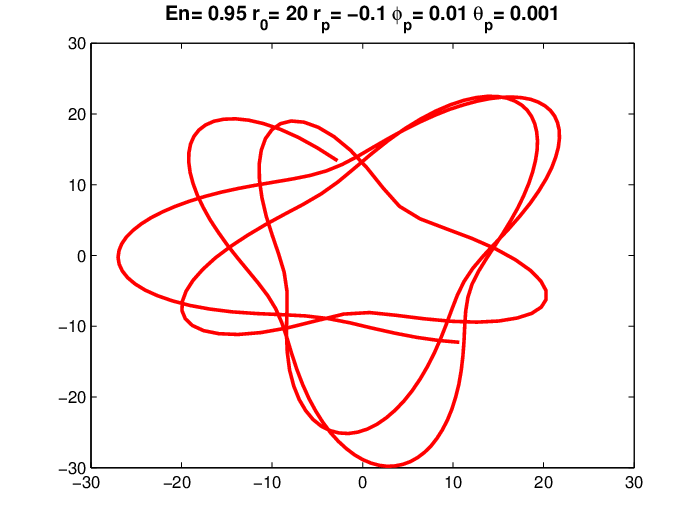
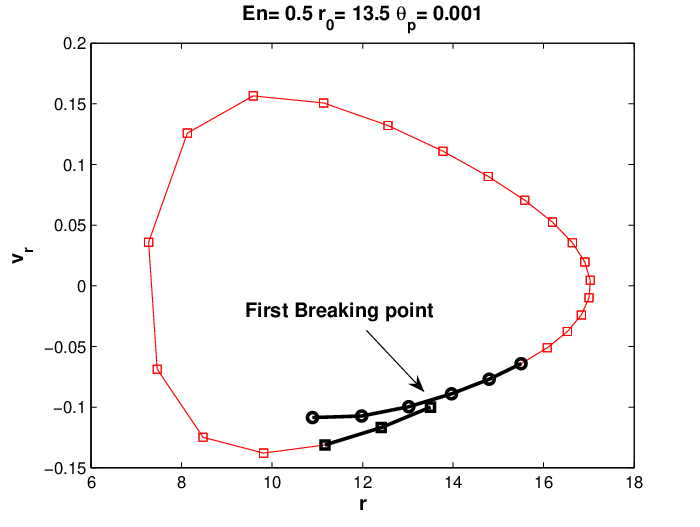
We have used for the computation the $6^{th}$ version of Wolfram Software Mathematica package [56]. The stiffness of the differential equations is evident from Fig. 1, where the first and second derivative of $r$, plotted with respect to $t$, show steep peaks corresponding to the points where the radial velocity changes its sign abruptly. We show the time series of both $\dot{r}(t)$ and $r(t)$ together with the phase portrait $\dot{r}=f(r)$ and $\ddot{r}(t)$, assuming given initial values for the angular precession and nutation velocities (see also Fig. 5. In Fig.1, the results for a given value of nutation angular velocity with a time span of $10000$ steps is shown. It is interesting to see that, by increasing the initial nutation angular velocity, being fixed all the other initial conditions, we get curves with decreasing frequencies for $\dot{r}(t)$ and $\ddot{r}(t)$. This fact is relevant to have an insight on the orbital motion stability (see Fig.4). We have taken into account the effect of gravitomagnetic terms, in Fig. 2, showing the basic orbits (left) and the orbit with the associated velocity field in false colors (right). From a rapid inspection of the right panel, it is clear the sudden changes of velocity direction induced by the gravitomagnetic effects.

To show the orbital velocity field, we have performed a rotation and a projection of the orbits along the axes of maximal energy. In other words, by a Singular Value Decomposition of the de-trended positions and velocities, we have selected only the eigenvectors corresponding to the largest eigenvalues and, of course, those representing the highest energy components (see Fig 2).

The above differential equations for the parametric orbital motion are non-linear and with time-varying coefficients. In order to have a well-posed Cauchy problem, we have to define:

• •

  the initial and final boundary condition problems;

• •

  the stability and the dynamical equilibrium of solutions.

We can start by solving the Cauchy problem, as in the classical case, for the initial condition putting $\dot{r}=0$ , $\dot{\phi}=0$, $\dot{\theta}=0$ and $\theta=\frac{\pi}{2}$ and the result we get is that the orbit is not planar being $\ddot{\theta}\neq 0$. In this case, we are compelled to solve numerically the system of second order differential equations and to treat carefully the initial conditions, taking into account the high non-linearity of the system. A similar discussion, but for different problems, can be found in [57, 58].

A series of numerical trials on the orbital parameters can be done in order to get an empirical insight on the orbit stability. The parameters involved in this analysis are the mass, the energy, the orbital radius, the initial values of $r,\phi,\theta$ and the angular precession and nutation velocities $\dot{\phi}$ and $\dot{\theta}$ respectively. We have empirically assumed initial conditions on $\dot{r}$, $\dot{\phi}$ and $\dot{\theta}$.

The trials we have performed can be organized in two series, i.e. constant mass and energy variation and constant energy and mass variation.

• •

  In the first class of trials, we assume the mass equal to $M=1M_{\bigodot}$ and the energy $E_{n}$ (in mass units) varying step by step. The initial orbital radius $r_{0}$ can be changed, according to the step in energy: this allow to find out numerically the dynamical equilibrium of the orbit. We have also chosen, as varying parameters, the ratios of the precession angular velocity $\dot{\phi}$ to the radial angular velocity $\dot{r}$ and the ratio of the nutation angular velocity $\dot{\theta}$ and the precession angular velocity $\dot{\phi}$. The initial condition on $\phi$ has been assumed to be $\phi_{0}=0$ and the initial condition on $\theta$ has been $\theta_{0}=\frac{\pi}{2}$. For $M=1$ (in Solar masses) , $\frac{\dot{\theta}}{\dot{\phi}}=\frac{1}{2}$ and $\dot{\phi}=-\frac{\dot{r}}{10}$, we have found out two different empirical linear equations, according to the different values of $\dot{\theta},\dot{\phi}$. We obtain a rough guess of the initial distance $r_{0}=r_{0}(E_{n})$ around which is possible to find a guess on the equilibrium of the initial radius, followed by trials and errors procedure.

• •

  In the second class of trials, we have assumed the variation of the initial orbital radius for different values of mass at a constant energy value equal to $E_{n}=0.95$ in mass units. With this conditions, we assume ${\displaystyle\dot{\phi}=\frac{\dot{r}}{10}}$ and assume that $\dot{\theta}$ takes the two values $1/2$ and $1/10$. We can approach the problem also considering the mass parameterization, at a given fixed energy, to have an insight of the effect of mass variation on the initial conditions. The masses have been varied between 0.5 and 20 Solar masses and the distances have been found to vary according to the two 3rd-order polynomial functions, according to the different values of $\dot{\theta}$ with respect to the mass.

In summary, the numerical calculations, if optimized, allow to put in evidence the specific contributions of gravitomagnetic corrections on orbital motion. In particular, specific contributions due to nutation and precession emerge when higher order terms in $v/c$ are considered.

In this paper, we have discussed the theory of orbits considering gravitomagnetic effects in the geodesic motion. In particular, we have considered the orbital effects of higher-order terms in $v/c$ which is the main difference with respect to the standard approach to the gravitomagnetism. Such terms are often discarded but, as we have shown, they could give rise to interesting phenomena in tight binding systems as binary systems of evolved objects (neutron stars or black holes). They could be important for objects falling toward extremely massive black holes as those seated in the galactic centers [57, 58]. The leading parameter for such correction is the ratio $v/c$ which, in several physical cases cannot be simply discarded. For a detailed discussion see for example [26, 27, 28, 30]. A part the standard periastron precession effects, such terms induce nutations and are capable of affecting the stability basin of the orbital phase space. As shown, the global structure of such a basin is extremely sensitive to the initial angular velocities, the initial energy and mass conditions which can determine possible transitions to chaotic behaviors. Detailed studies on the transition to chaos could greatly aid in gravitational wave detections in order to determine the shape, the spectrum and the intensity of the waves (for a discussion see [59, 60]).

In a forthcoming paper, we will discuss how gravitomagnetic effects could affect also the gravitational wave production in extreme gravitational field regimes.

References

- [1] J.C. Maxwell,Phil. Trans., 155, (1865) 492.
- [2] G. Holzmuller, Z. Math. Phys 15, (1870) 69.
- [3] F. Tisserand, Compte Rendu hebdomadaire des scéances de L’Acad’emie des Sciences, 75, (1872) 760; 110, (1890) 313.
- [4] J.D.North, The Measure of the Universe, Dover Publications, New York, (1989).
- [5] E. Whittaker, A History of the Theories of Aether and Electricity, Vol. I: The Classical Theories, Harper and Brothers, New York (1960).
- [6] O. Heaviside, Electromagnetic Theory, The Electrician Printing and Publishing Co., London (1894).
- [7] O. Heaviside, The Electrician, 31 (1893) 281.
- [8] A. Einstein, Phys. Z. 14 (1913) 1261.
- [9] H. Thirring, Phys. Z. 19 (1918) 204.
- [10] H. Thirring, Phys. Z. 19 (1918) 33; J. Lense and H. Thirring, Phys. Z. 19 (1918) 156; B. Mashhoon, F.W. Hehl and D.S. Theiss, Gen. Rel. Grav. 16 (1984) 711.
- [11] H. Pfister, Gen. Rel. Grav. 39 (2007) 1735.
- [12] R. Anderson, H.R. Bilger and G.E. Stedman, Am. J. Phys. 62 (1994) 975.
- [13] L. Cugusi and E. Proverbio Astron. & Astrophys. 69 (1978) 321.
- [14] L. Iorio, Scholarly Research Exchange (2008) 105235.
- [15] L. Iorio, Class. Quant. Grav. 23 (2006) 5451; K. Krogh, Class. Quant. Grav. 24 (2007) 5709.
- [16] L. Iorio and V. Lainey, Int. Jou. Mod. Phys. D 14 (2005) 2039.
- [17] J.C. Ries, R.J. Eanes, and M.M. Watkins, Confirming the Frame-Dragging Effect with Satellite Laser Ranging, 16th Int. Laser Ranging Workshop, Poznan (PL) 13-17 October 2008.
- [18] L. Iorio, Adv. Space. Res. doi:10.1016/j.asr.2008.10.016.
- [19] C.W.F. Everitt et al., Near Zero: Festschrift for William M. Fairbank, ed. C.W.F. Everitt, Freeman Ed., S. Francisco (1986).
- [20] G.E. Pugh, Proposal for a Satellite Test of the Coriolis Prediction of General Relativity, WSEG Research Memorandum No. 11, reprinted in R. Ruffini and C. Sigismondi (eds) 2003, Nonlinear Gravitodynamics. The Lense-Thirring Effect Singapore, World Scientific, pp. 414-426.
- [21] L. Schiff, Phys. Rev. Lett. 4 (1960) 215.
- [22] Gravity Probe B Testing Einstein’s Universe, http://einstein.stanford.edu/
- [23] F. Gronwald, E. Gruber, H.I.M. Lichtenegger and R.A. Puntigam, Proceedings of the Alpbach Summer School 1997, Fundamental Physics in Space, Organized by the Austrian and European Space Agency, ed. A. Wilson, gr-qc/9712054.
- [24] B. Mashhoon, L. Iorio, and H.I.M. Lichtenegger, Phys. Lett. A 292 (2001) 49.
- [25] L. Iorio, and H.I.M. Lichtenegger, Class. Quant. Grav. 22 (2005) 119.
- [26] S. Capozziello, G. Lambiase, G. Papini, G. Scarpetta, Phys. Lett. A 254 (1999) 11.
- [27] S. Capozziello, V. Re, Phys. Lett. A 290 (2001) 115.
- [28] S. Capozziello, V.F. Cardone, V. Re, M. Sereno, Mon. Not. R. Ast. Soc. 343 (2003) 360.
- [29] S. Kopeikin and B. Mashhoon, Phys. Rev. 65 (2002) 064025.
- [30] M. Sereno and V.F. Cardone, Astron. & Astroph. 396 (2002) 393.
- [31] M. Sereno, Mon. Not. R. Ast. Soc. 3434 (2003) 942.
- [32] M. Sereno, Mon. Not. R. Ast. Soc. 356 (2005) 381.
- [33] B.J. Ahmedov, Phys. Lett. A 256 (1999) 9.
- [34] B.J. Ahmedov and N.I. Rakhmatov Found. of Phys. 33 (2003) 625.
- [35] L.Iorio, Class. Quant. Grav. 21 (2004) 2065.
- [36] L. Iorio, New Astronomy 14 (2009) 40.
- [37] R.M. Wald, Black Holes and Relativistic Stars Univ. Chicago Press, Chicago (1998).
- [38] J. Kormendy and D. O. Richstone, Ann. Rev. Astron. Astrophys., 33 (1995) 581.
- [39] S. Sigurdsson and M. Rees, Mont. Not. R. Astron. Soc., 284 (1997) 318.
- [40] S. Sigurdsson, Class. Quant. Grav. 14 (1997) 1425.
- [41] L. Iorio (ed.), The Measurement of Gravitomagnetism: A Challenging Enterprise, NOVA Science (2007), Hauppauge, New York.
- [42] R. Ruffini and C. Sigismondi, Nonlinear Gravitodynamics: The Lense-Thirring Effect, World Scientific (2003) Singapore.
- [43] L. Landau and E.M. Lifsits, Field Theory, Pergamon Press, New York (1973).
- [44] J.Binney and S.Tremaine, Galactic Dynamics, Princeton University Press, Princeton, New Jersey (1987).
- [45] W.M. Smart, Textbook on Spherical Astronomy, Cambridge University Press, Cambridge (1977).
- [46] B.M. Barker and R.F. O’Connell, Phys. Rev. D 10 (1974) 1340.
- [47] N. Ashby and T. Allison, Celest. Mech. Dyn. Astron. 57 (1993) 537.
- [48] L.Iorio, Nuovo Cim. B 116 (2001) 777.
- [49] M. L. Ruggiero, A. Tartaglia, Nuovo Cim. B 117 (2002) 743; Tartaglia A., Eur. J. Phys. 22 (2001) 105.
- [50] J.-F. Pascual-Sanchez Int. Jou. Mod. Phys. D 13 (2006) 2345.
- [51] S.M. Kopeikin Int. Jou. Mod. Phys. D 15 (2006) 305.
- [52] S. Weinberg, Gravitation and Cosmology, Wiley, New York (1972).
- [53] A. Roy, Orbital Motion, Fourth Edition IoP (2005) Bristol.
- [54] V. Brumberg, Essential Relativistic Celestial Mechanics , Taylor & Francis (1991) New York.
- [55] L. Landau and E.M. Lifsits, Mechanics, Pergamon Press, New York (1973).
- [56] http://www.wolfram.com
- [57] L. Barack and C. Cutler, Phys. Rev. D 69 (2004). 082005.
- [58] L. Barack and C. Cutler, Phys. Rev. D 70 (2004) 122002.
- [59] J. Levin, arXiv: gr-qc/9910040 (2000).
- [60] J.R. Gair et al., Class. Quant. Grav. 21 (2004) S1595.