The Offset Tree for Learning with Partial LabelsThanks: work done while at IBM ResearchThanks: work done while at Yahoo! Research
Abstract
We present an algorithm, called the , for learning to make decisions in situations where the payoff of only one choice is observed, rather than all choices. The algorithm reduces this setting to binary classification, allowing one to reuse of any existing, fully supervised binary classification algorithm in this partial information setting. We show that the Offset Tree is an optimal reduction to binary classification. In particular, it has regret at most times the regret of the binary classifier it uses (where is the number of choices), and no reduction to binary classification can do better. This reduction is also computationally optimal, both at training and test time, requiring just work to train on an example or make a prediction.
Experiments with the show that it generally performs better than several alternative approaches.
1 Introduction
This paper is about learning to make decisions in partial feedback settings where the payoff of only one choice is observed rather than all choices.
As an example, consider an internet site recommending ads or other content based on such observable quantities as user history and search engine queries, which are unique or nearly unique for every decision. After the ad is displayed, a user either clicks on it or not. This type of feedback differs critically from the standard supervised learning setting since we don’t observe whether or not the user would have clicked had a different ad beed displayed instead.
In an online version of the problem, a policy chooses which ads to display and uses the observed feedback to improve its future ad choices. A good solution to this problem must explore different choices and properly exploit the feedback.
The problem faced by an internet site, however, is more complex. They have observed many interactions historically, and would like to exploit them in forming an initial policy, which may then be improved by further online exploration. Since exploration decisions have already been made, online solutions are not applicable. To properly use the data, we need non-interactive methods for learning with partial feedback.
This paper is about constructing a family of algorithms for non-interactive learning in such partial feedback settings. Since any non-interactive solution can be composed with an exploration policy to form an algorithm for the online learning setting, the algorithm proposed here can also be used online. Indeed, some of our experiments are done in an online setting.
Problem Definition
Here is a formal description of non-interactive data generation:
- 1.
Some unknown distribution generates a feature vector and a vector , where is the reward of the -th action, . Only is revealed to the learner.
- 2.
An existing policy chooses an action .
- 3.
The reward is revealed.
The goal is to learn a policy for choosing action given , with the goal of maximizing the expected reward with respect to , given by
We call this a partial label problem (defined by) .
Existing Approaches
Probably the simplest approach is to regress on the reward given and , and then choose according to the largest predicted reward given a new . This approach reduces the partial label problem to a standard regression problem.
A key technique for analyzing such a reduction is regret analysis, which bounds the “regret” of the resulting policy in terms of the regressor’s “regret” on the problem of predicting given and . Here regret is the difference between the largest reward that can be achieved on the problem and the reward achieved by the predictor; or—defined in terms of losses—the difference between the incurred loss and the smallest achievable loss. One analyzes excess loss (i.e., regret) instead of absolute loss so that the bounds apply to inherently noisy problems. It turns out that the simple approach above has regret that scales with the square root of the regressor’s regret (see section 6 for a proof). Recalling that the latter is upper bounded by 1, this is undesirable.
Another natural approach is to use the technique in [25]. Given a distribution over the actions given , the idea is to transform each partial label example into an importance weighted multiclass example , where is the cost of not predicting label on input . These examples are then fed into any importance weighted multiclass classification algorithm, with the output classifier used to make future predictions. Section 6 shows that when is uniform, the resulting regret on the original partial label problem is bounded by times the importance weighted multiclass regret, where is the number of choices. The importance weighted multiclass classification problem can, in turn, be reduced to binary classification, but all known conversions yield worse bounds than the approach presented in this paper.
Results
We propose the algorithm for reducing the partial label problem to binary classification, allowing one to reuse any existing, fully supervised binary classification algorithm for the partial label problem.
The uses the following trick, which is easiest to understand in the case of choices (covered in section 3). When the observed reward of choice is low, we essentially pretend that the other choice was chosen and a different reward was observed. Precisely how this is done and why, is driven by the regret analysis. This basic trick is composable in a binary tree structure for , as described in section 4.
The achieves computational efficiency in two ways: First, it improves the dependence on from to . It is also an oracle algorithm, which implies that it can use the implicit optimization in existing learning algorithms rather than a brute-force enumeration over policies, as in the Exp4 algorithm [3]. We prove that the policy regret is bounded by times the regret of the binary classifier in solving the induced binary problems. Section 5 shows that no reduction can provide a better guarantee, giving the first nontrivial lower bound for learning reductions. Since the bound is tight and has a dependence on , it shows that the partial label problem is inherently different from standard fully supervised learning problems like -class classification.
Related Work
The problem considered here is a non-interactive version of the contextual bandit problem (see [2, 3, 8, 19, 24] for background on the bandit problem). The interactive version has been analyzed under various additional assumptions [7, 13, 17, 18, 20, 22], including payoffs as a linear function of the side information [1, 2]. The Exp4 algorithm [3] has a nice assumption-free analysis. However, it is intractable when the number of policies we want to compete with is large. It also relies on careful control of the action choosing distribution, and thus cannot be applied to historical data, i.e., non-interactively.
Sample complexity results for policy evaluation in reinforcement learning [12] and contextual bandits [17] show that Empirical Risk Minimization type algorithms can find a good policy in a non-interactive setting. The results here are mostly orthogonal to these results, although we do show in section A that a constant factor improvement in sample complexity is possible using the offset trick.
The Banditron algorithm [7] deals with a similar setting but does not address several concerns that the addresses: (1) the Banditron requires an interactive setting; (2) it deals with a specialization of our setting where the reward for one choice is , and for all other choices; (3) its analysis is further specialized to the case where linear separators with a small hinge loss exist; (4) it requires exponentially in more computation; (5) the Banditron is not an oracle algorithm, so it is unclear, for example, how to compose it with a decision tree bias.
Transformations from partial label problems to fully supervised problems can be thought of as learning methods for dealing with sample selection bias [11], which is heavily studied in Economics and Statistics.
2 Basic Definitions
This section reviews several basic learning problems and the method [26] used in the construction.
A -class classification problem is defined by a distribution over , where is an arbitrary feature space and is a label space with . The goal is to learn a classifier minimizing the error rate on ,
given training examples of the form . Here is the indicator function which evaluates to 1 when its argument is true, and to 0 otherwise.
Importance weighted classification is a generalization where some errors are more costly than others. Formally, an importance weighted classification problem is defined by a distribution over . Given training examples of the form , where is the cost associated with mislabeling , the goal is to learn a classifier minimizing the importance weighted loss on , .
A folk theorem [26] says that for any importance weighted distribution , there exists a constant such that for any classifier ,
where is the distribution over defined by
marginalized over . In other words, choosing to minimize the error rate under is equivalent to choosing to minimize the importance weighted loss under .
The method [26] can be used to resample the training set drawn from using rejection sampling on the importance weights (an example with weight is accepted with probability proportional to ), so that the resampled set is effectively drawn from . Then, any binary classification algorithm can be run on the resampled set to optimize the importance weighted loss on .
runs a base classification algorithm on multiple draws of the resampled set, and averages over the learned classifiers when making importance weighted predictions (see [26] for details). To simplify the analysis, we do not actually have to consider separate classifiers. We can simply augment the feature space with the index of the resampled set and then learn a single classifier on the union of all resampled data. The implication of this observation is that we can view as a machine that maps importance weighted examples to unweighted examples. We use this method in Algorithms 1 and 2 below.
3 The Binary Case
This section deals with the special case of actions. We state the algorithm, prove the regret bound (which is later used for the general case), and state a sample complexity bound. For simplicity, we let the two action choices in this section be and .
3.1 The Algorithm
The algorithm is a reduction from the 2-class partial label problem to binary classification. The reduction operates per example, implying that it can be used either online or offline. We state it here for the offline case. The algorithm reduces the original problem to binary importance weighted classification, which is then reduced to binary classification using the method described above. A base binary classification algorithm is used as a subroutine.
The key trick appears inside the loop in Algorithm 1, where importance weighted binary examples are formed. The offset of changes the range of importances, effectively reducing the variance of the induced problem. This trick is driven by the regret analysis in section 3.2.
3.2 Regret Analysis
This section proves a regret transform theorem for the reduction. Informally, regret measures how well a predictor performs compared to the best possible predictor on the same problem. A regret transform shows how the regret of a base classifier on the induced (binary classification) problem controls the regret of the resulting policy on the original (partial label) problem. Thus a regret transform bounds only excess loss due to suboptimal prediction.
transforms partial label examples into binary examples. This process implicitly transforms the distribution defining the partial label problem into a distribution over binary examples, via a distribution over importance weighted binary examples. Note that even though the latter distribution depends on both and the action-choosing distribution , the induced binary distribution depends only on . Indeed, the unnormalized probability of label 1 given and , according to , is
independent of .
The binary regret of a classifier on is given by
where the min is over all classifiers . The importance weighted regret is definited similarly with respect to the importance weighted loss.
For the partial label case, the policy that a classifier induces is simply the classifier. The regret of policy is defined as
where
is the value of the policy.
The theorem below states that the policy regret is bounded by the binary regret. We find it surprising because strictly less information is available than in binary classification. Note that the lower bound in section 5 implies that no reduction can do better. Redoing the proof with the offset set to rather than also reveals that bounds the policy regret, implying that the offset trick gives a factor of 2 improvement in the bound.
Finally, note that the theorem is quantified over all classifiers, which includes the classifier returned by in the last line of the algorithm.
Theorem 3.1.
( Regret) For all -class partial label problems and all binary classifiers ,
Furthermore, the bound is tight: There exists a distribution such that, for any value , there exists a classifier satisfying .
Proof.
We first bound the partial label regret of in terms of importance weighted regret, and then apply known results to relate the importance weighted regret to binary regret.
Condition what follows on a fixed , taking the expectation over at the end. We can assume without loss of generality that . If , the regrets on both sides are , and the claim holds trivially. Otherwise, makes a mistake on .
The importance-weighted error of predicting on is given by
where expectations and probabilities are with respect to .
Similarly, the error of predicting on is
The importance-weighted regret of preferring to on is given by the difference of the two expressions above. As the four -terms cancel out, the importance-weighted regret simplifies to
Thus the importance weighted regret of the binary classifier is the policy regret. The folk theorem from section 2 (see [26]) says that the importance weighted regret is bounded by the binary regret, times the expected importance. The latter is
since both and are bounded by 1. Taking expectation over finishes the first part of the theorem.
For the second part, notice that the proof of the first part can be made an equality by having a reward vector for each always, and letting the classifier predict label with probability over the draw of . ∎
4 The Offset Tree Reduction
In this section we deal with the case of large .
4.1 The Offset Tree Algorithm
The technique in the previous section can be applied repeatedly using a tree structure to give an algorithm for general . Consider a maximally balanced binary tree on the set of choices, conditioned on a given observation . Every internal node in the tree is associated with a classification problem of predicting which of its two inputs has the larger expected reward. At each node, the same offsetting technique is used as in the binary case described in section 3.
For an internal node , let denote the set of leaves in the subtree rooted at . Every input to a node is either a leaf or a winning choice from another internal node closer to the leaves.
The training algorithm, , is given in Algorithm 2. The testing algorithm defining the predictor is given in Algorithm 3.
4.2 The Offset Tree Regret Theorem
The theorem below gives an extension of Theorem 3.1 for general . For the analysis, we use a simple trick which allows us to consider only a single induced binary problem, and thus a single binary classifier . The trick is to add the node index as an additional feature into each importance weighted binary example created algorithm 2, and then train based upon the union of all the training sets.
As in section 3, the reduction transforms a partial label distribution into a distribution over binary examples. To draw from , we draw from , an action from the action-choosing distribution , and apply algorithm 2 to transform into a set of binary examples (up to one for each level in the tree) from which we draw uniformly at random. Note that is independent of , as explained in the beginning of section 3.
Denote the policy induced by the Offset-Test algorithm using classifier by . For the following theorem, the definitions of regret are from section 3.
Theorem 4.1.
( Regret) For all -class partial label problems , for all binary classifiers ,
where ranges over the internal nodes in , and and are its inputs determined by ’s predictions.
Note: Section 5 shows that no reduction can give a better regret transform theorem. With a little bit of side information, however, we can do better: The offset minimizing the regret bound turns out to be the median value of the reward given . Thus, it is generally best to pair choices which tend to have similar rewards. Note that the algorithm need not know how well performs on .
The proof below can be reworked with the offset set to , resulting in a regret bound which is a factor of worse.
Proof.
We fix , taking the expectation over the draw of at the end. The first step is to show that the partial label regret is bounded by the sum of the importance weighted regrets over the binary prediction problems in the tree. We then apply the costing analysis [26] to bound this sum in terms of the binary regret.
The proof of the first step is by induction on the nodes in the tree. We want to show that the sum of the importance weighted regrets of the nodes in any subtree bounds the regret of the output choice for the subtree. The hypothesis trivially holds for one-node trees.
Consider a node making an importance weighted decision between choices and . Without loss of generality, has the larger expected reward. As shown in the proof of Theorem 3.1, the importance weighted binary regret of the classifier’s decision at is either if it predicts , or if it predicts .
Let be the subtree rooted at node , and let be the choice output by on . If the best choice in comes from the subtree producing , the policy regret of is given by
If on the other hand the best choice comes from the other subtree , we have
proving the induction.
The induction hypothesis applied to tells us that . According to the Costing theorem discussed in section 2, the importance weighted regret is bounded by the unweighted regret on the resampled distribution, times the expected importance. The expected importance of deciding between actions and is
since all rewards are between 0 and 1. Noting that , we thus have
completing the proof for any . Taking the expectation over finishes the proof. ∎
The setting above is akin to Boosting [9]: At each round , a booster creates an input distribution and calls an oracle learning algorithm to obtain a classifier with some error on . The distribution depends on the classifiers returned by the oracle in previous rounds. The accuracy of the final classifier is analyzed in terms of ’s. The binary problems induced at internal nodes of an offset tree depend, similarly, on the classifiers closer to the leaves. The performance of the resulting partial label policy is analyzed in terms of the oracle’s performance on these problems. (Notice that Theorem 4.1 makes no assumptions on the error rates on the binary problems; in particular, it doesn’t require them to be bounded away from .)
For the analysis, we use the simple trick from the beginning of this subsection to consider only a single binary classifier. The theorem is quantified over all classifiers, and thus it holds for the classifier returned by the algorithm. In practice, one can either call the oracle multiple times to learn a separate classifier for each node (as we do in our experiments), or use iterative techniques for dealing with the fact that the classifiers are dependent on other classifiers closer to the leaves.
5 A Lower Bound
This section shows that no method for reducing the partial label setting to binary classification can do better. First we formalize a learning reduction which relies upon a binary classification oracle. The lower bound we prove below holds for all such learning reductions.
Definition 5.1.
(Binary Classification Oracle) A binary classification oracle is a (stateful) program that supports two kinds of queries:
- 1.
Advice. An advice query consists of a single example , where is a feature vector and is a binary label. An advice query is equivalent to presenting the oracle with a training example, and has no return value.
- 2.
Predict. A predict query is made with a feature vector . The return value is a binary label.
All learning reductions work on a per-example basis, and that is the representation we work with here.
Definition 5.2.
(Learning Reduction) A learning reduction is a pair of algorithms and .
- 1.
The algorithm takes a partially labeled example and a binary classification oracle as input, and forms a (possibly dependent) sequence of advice queries.
- 2.
The algorithm takes an unlabeled example and a binary classification oracle as input. It asks a (possibly dependent) sequence of predict queries, and makes a prediction dependent only on the oracle’s predictions. The oracle’s predictions may be adversarial (and are assumed so by the analysis).
We are now ready to state the lower bound.
Theorem 5.1.
For all reductions , there exists a partial label problem and an oracle such that
where is the binary distribution induced by on , and is the policy resulting from using .
Proof.
The proof is by construction. We choose to be uniform over examples, with example having 1 in its -th component of the reward vector, and zeros elsewhere. The corresponding feature vector consists of the binary representation of the index with reward 1. Let the action-choosing distribution be uniform.
The reduction produces some simulatable sequence of advice calls when the observed reward is 0. The oracle ignores all advice calls from and chooses to answer all queries with zero error rate according to this sequence.
There are two cases: Either observes reward (with probability ) or it observes reward (with probability ). In the first case, the oracle has error rate (and, hence regret). In the second case, it has error rate (and regret) of at most . Thus the expected error rate of the oracle on is at most .
The inverse reduction has access to only the unlabeled example and the oracle . Since the oracle’s answers are independent of the draw from , the output action has reward with probability and reward with probability , implying a regret of with respect to the best policy. This is a factor of greater than the regret of the oracle, proving the lower bound. ∎
6 Analysis of Simple Reductions
This section analyzes two simple approaches for reducing partial label problems to basic supervised learning problems. These approaches have been discussed previously, but the analysis is new.
6.1 The Regression Approach
The most obvious approach is to regress on the value of a choice as in Algorithm 4, and then use the argmax classifier as in Algorithm 5. Instead of learning a single regressor, we can learn a separate regressor for each choice.
The squared error of a regressor on a distribution over is denoted by
The corresponding regret is given by .
The following theorem relates the regret of the resulting predictor to that of the learned regressor.
Theorem 6.1.
For all -class partial label problems and all squared-error regressors ,
where is the regression distribution induced by Algorithm 4 on , and is the argmax policy based on . Furthermore, there exist and such that the bound is tight.
The theorem has a square root, which is undesirable, because the theorem is vacuous when the right hand side is greater than 1.
Proof.
Let choose some action with true value . Some other action may have a larger expected reward . The squared error regret suffered by on is . Similarly for , we have regret . In order for to be chosen over , we must have . Convexity of the two regrets implies that the minima is reached when , where the regret for each of the two choices is . The regressor need not suffer any regret on the other arms. Thus with average regret a regret of can be induced, completing the proof of the first part. For the second part, note that an adversary can play the optimal strategy outlined above achieving the bound precisely. ∎
6.2 Importance Weighted Classification
Zadrozny [25] noted that the partial label problem could be reduced to importance weighted multiclass classification. After Algorithm 6 creates importance weighted multiclass examples, the weights are stripped using Costing (the rejection sampling on the weights discussed in Section 2), and then the resulting multiclass distribution is converted into a binary distribution using, for example, the all-pairs reduction [10]). The last step is done to get a comparable analysis.
All-Pairs-Train uses a given binary learning algorithm Learn to distinguish each pair of classes in the multiclass distribution created by Costing. The learned classifier predicts, given and a distinct pair of classes , whether class is more likely than given . At test time, we make a choice using All-Pairs-Test, which takes and an unlabeled example , and returns the class that wins the most pairwise comparisons on , according to .
A basic theorem applies to this approach.
Theorem 6.2.
For all -class partial label problems and all binary classifiers ,
where is the IWC-Test policy based on and is the binary distribution induced by IWC-Train on .
Proof.
The proof first bounds the policy regret in terms of the importance weighted multiclass regret. Then, we apply known results for the other reductions to relate the policy regret to binary classification regret.
Fix a particular . The policy regret of choosing action over the best action is . The importance weighted multiclass loss of action is
since the loss is proportional to with probability . This implies the importance weighted regret of
which is the same as the policy regret.
Relative to the , this theorem has an undesirable extra factor of in the regret bound. While this factor is due to the all-pairs reduction being a weak regret transform, we are aware of no alternative approach for reducing multiclass to binary classification that in composition can yield the same regret transform as the .
7 Experimental Results
| Properties | Single regressor | regressors | ||||||
|---|---|---|---|---|---|---|---|---|
| Dataset | Weighting | M5P | REPTree | M5P | REPTree | Offset Tree | ||
| ecoli | 8 | 336 | 0.3120 | 0.5663 | 0.3376 | 0.3752 | 0.3811 | 0.2311 |
| flare | 7 | 1388 | 0.1565 | 0.1570 | 0.1685 | 0.1570 | 0.1592 | 0.1506 |
| glass | 6 | 214 | 0.5938 | 0.6662 | 0.5846 | 0.5800 | 0.6077 | 0.5000 |
| letter | 25 | 20000 | 0.3546 | 0.6974 | 0.5491 | 0.4456 | 0.5352 | 0.3790 |
| lymph | 4 | 148 | 0.2953 | 0.5267 | 0.4622 | 0.3422 | 0.3400 | 0.3114 |
| optdigits | 10 | 5620 | 0.1682 | 0.5426 | 0.4108 | 0.1948 | 0.2956 | 0.1649 |
| page-blocks | 5 | 5473 | 0.0407 | 0.0590 | 0.0451 | 0.0571 | 0.0465 | 0.0488 |
| pendigits | 10 | 10992 | 0.1029 | 0.2492 | 0.1840 | 0.1408 | 0.1774 | 0.0976 |
| satimage | 6 | 6435 | 0.1703 | 0.2027 | 0.1968 | 0.1787 | 0.1878 | 0.1853 |
| soybean | 19 | 683 | 0.6533 | 0.8824 | 0.7327 | 0.7688 | 0.7473 | 0.5971 |
| vehicle | 4 | 846 | 0.3719 | 0.6142 | 0.5665 | 0.3886 | 0.4114 | 0.3743 |
| vowel | 11 | 990 | 0.6403 | 0.9034 | 0.8919 | 0.7440 | 0.8198 | 0.6501 |
| yeast | 10 | 1484 | 0.5406 | 0.6626 | 0.5679 | 0.5406 | 0.5697 | 0.4904 |
We conduct two sets of experiments. The first set compares the Offset Tree with the two approaches from section 6. The second compares with the Banditron [7] on the dataset used in that paper.
7.1 Comparisons with Reductions
Ideally, this comparison would be with a data source in the partial label setting. Unfortunately, data of this sort is rarely available publicly, so we used a number of publicly available multiclass datasets [21] and allowed queries for the reward ( or for correct or wrong) of only one value per example.

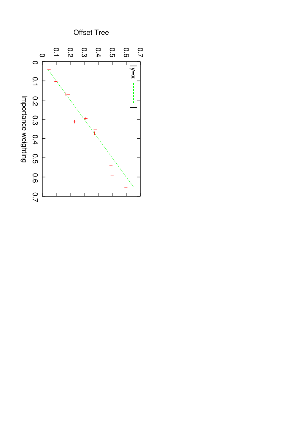
For all datasets, we report the average result over 10 random splits (fixed for all methods), with of the dataset used for training and for testing. Figure 1 shows the error rates (in %) of the plotted against the error rates of the regression (left) and the importance weighting (right). Decision trees (J48 in Weka [23]) were used as a base binary learning algorithm for both the and the importance weighting. For the regression approach, we learned a separate regressor for each of the choices. (A single regressor trained by adding the choice as an additional feature performed worse.) M5P and REPTree, both available in Weka [23], were used as base regression algorithms.
The clearly outperforms regression, in some cases considerably. The advantage over importance weighting is moderate: Often the performance is similar and occasionally it is substantially better.
We did not perform any parameter tuning because we expect that practitioners encountering partial label problems may not have the expertise or time for such optimization. All datasets tested are included. Note that although some error rates appear large, we are choosing among alternatives and thus an error rate of less than gives an advantage over random guessing. Dataset-specific test error rates are reported in Table 1.
7.2 Comparison with the Banditron Algorithm
The Banditron [7] is an algorithm for the special case of the problem where one of the rewards is and the rest are . The sample complexity guarantees provided for it are particularly good when the correct choice is separated by a multiclass margin from the other classes.
We chose the Binary Perceptron as a base classification algorithm since it is the closest fully supervised learning algorithm to the Banditron. Exploration was done according to Epoch-Greedy [17] instead of Epsilon-Greedy (as in the Banditron), motivated by the observation that the optimal rate of exploration should decay over time. The Banditron was tested on one dataset, a 4-class specialization of the Reuters RCV1 dataset consisting of 673,768 examples. We use precisely the same dataset, made available by the authors of [7].
Since the Banditron analysis suggests the realizable case, and the dataset tested on is nearly perfectly separable, we also specialized the for the realizable case. In particular, in the realizable case we can freely learn from every observation implying it is unnecessary to importance weight by . We also specialize Epoch-Greedy to this case by using a realizable bound, resulting in a probability of exploration that decays as rather than .
The algorithms are compared according to their error rate. For the Banditron, the error rate after one pass on the dataset was . For the realizable method above, the error rate was . For the fully agnostic version of the , the error rate was . These results suggest there is some tradeoff between being optimal when there is arbitrary noise, and performance when there is no or very little noise. In the no-noise situation, the realizable performs substantially superior to the Banditron.
8 Discussion
We have analyzed the tractability of learning when only one outcome from a set of alternatives is known, in the reductions setting. The approach has a worst-case dependence on (Theorem 4.1), and no other reduction approach can provide a better guarantee (Section 5). Furthermore, with an computation, the is qualitatively more efficient than all other known algorithms, the best of which are . Experimental results suggest that this approach is empirically promising.
The algorithms presented here show how to learn from one step of exploration. By aggregating information over multiple steps, we can learn good policies using binary classification methods. A straightforward extension of this method to deeper time horizons is not compelling as is replaced by in the regret bounds. Due to the lower bound proved here, it appears that further progress on the multi-step problem in this framework must come with additional assumptions.
9 Acknowledgements
We would like to thank Tong Zhang, Alex Strehl, and Sham Kakade for helpful discussions. We would also like to thank Shai Shalev-Shwartz for providing data and helping setup a clean comparison with the Banditron.
References
- (1) N. Abe, A. Biermann, and P. Long. Reinforcement learning with immediate rewards and linear hypotheses, Algorithmica, 37(4): 263–293, 2003.
- (2) P. Auer. Using confidence bounds for exploitation-exploration tradeoffs, Journal of Machine Learning Research, 3: 397–422, 2002.
- (3) P. Auer, N. Cesa-Bianchi, Y. Freund, and R. Schapire. Gambling in a rigged casino: The adversarial multi-armed bandit problem, Proceedings of the 36th Annual Symposium on Foundations of Computer Science (FOCS), 322–331, 1995.
- (4) P. Auer, N. Cesa-Bianchi, and P. Fischer. Finite time analysis of the multi-armed bandit problem, Machine Learning, 47: 235–256, 2002.
- (5) B. Edelman, M. Ostrovsky and M. Schwarz. Internet Advertising and the Generalized Second-Price Auction: Selling Billions of Dollars Worth of Keywords, American Economic Review, Vol 97, 242–259, 2007.
- (6) B. Edelman and M. Schwarz. Optimal Auction design in a multi-unit environment: The case of sponsored search auctions.ACM Conference on Electronic Commerce, 2007.
- (7) S. Kakade, S. Shalev-Schwartz, and A. Tewari. Efficient bandit algorithms for online multiclass prediction, Proceedings of the 25th International Conference on Machine Learning (ICML), 2008.
- (8) E. Even-dar, S. Mannor, and Y. Mansour. Action elimination and stopping conditions for the multi-armed bandit and reinforcement learning problems, Journal of Machine Learning Research, 7: 1079–1105, 2006.
- (9) Y. Freund and R. Schapire. A decision-theoretic generalization of online learning and an application to boosting, Journal of Computer and System Sciences, 55(1): 119–139, 1997.
- (10) T. Hastie and R. Tibshirani. Classification by pairwise coupling, Annals of Statistics, 26(2): 451–471, 1998. (Also in Advances in Neural Information Processing Systems (NIPS), 10: 507–513, 1998.)
- (11) J. Heckman. Sample selection bias as a specification error, Econometrica, 47(1): 153–161, 1979.
- (12) M. Kearns, Y. Mansour, and A. Y. Ng. Approximate planning in large POMDPs via reusable trajectories, Advances in Neural Information Processing Systems (NIPS), 12, 2000.
- (13) S. Kulkarni. On bandit problems with side observations and learnability, Proceedings of the 31st Allerton Conference on Communication, Control, and Computing, 83–92, 1993.
- (14) J. Langford. Tutorial on practical prediction theory for classification, Journal of Machine Learning Research, 6(3): 273–306, 2005.
- (15) J. Langford and A. Beygelzimer. Sensitive error correcting output codes, Proceedings of the 18th Annual Conference on Learning Theory (COLT), 158–172, 2005.
- (16) J. Langford, L. Li, and A. Strehl. Vowpal Wabbit online learning software. Available at http://hunch.net/ vw, 2007.
- (17) J. Langford and T. Zhang. The Epoch-greedy algorithm for contextual multiarmed bandits, NIPS 2007.
- (18) S. Pandey, D. Agarwal, D. Chakrabati, V. Josifovski. Bandits for taxonomies: a model based approach, SDM 2007.
- (19) H. Robbins. Some aspects of the sequential design of experiments, Bulletins of the American Mathematical Society, 58: 527–535, 1952.
- (20) A. Strehl, C. Mesterham, M. Littman, and H. Hirsh. Experience-efficient learning in associative bandit problems, ICML 2006, 889–896.
- (21) Lichman, UCI Machine Learning Repository, Irvine, CA: University of California, School of Information and Computer Science, 2013.
- (22) C. C. Wang, S. Kulkarni, and H. Vincent Poor, Bandit problems with side observations, IEEE Transactions on Automatic Control, 50(5), 2005.
- (23) I. Witten and E. Frank. Data Mining: Practical machine learning tools with Java implementations, http://www.cs.waikato.ac.nz/ml/weka/, 2000.
- (24) M. Woodruff. A one-armed bandit problem with concomitant variates, JASA, 74 (368): 799–806, 1979.
- (25) B. Zadrozny, Ph.D. Thesis, University of California, San Diego, 2003.
- (26) B. Zadrozny, J. Langford, and N. Abe. Cost sensitive learning by cost-proportionate example weighting, Proceedings of the 3rd IEEE International Conference on Data Mining (ICDM), 435–442, 2003.
Appendix A Sample Complexity Bound
This section proves a simple sample complexity bound on the performance of . For ease of comparison with existing results, we specialize the problem set to partial label binary classification problems where one label has reward and the other label has reward . Note that this is not equivalent to assuming realizability: Conditioned on , any distribution over reward vectors and is allowed.
Comparing the bound with standard results in binary classification (see, for example, [14]), shows that the bounds are identical, while eliminating the offset trick weakens the performance by a factor of roughly 2.
When a sample set is used as a distribution, we mean the uniform distribution over the sample set (i.e., an empirical average).
Theorem A.1.
( Sample Complexity) Let the action choosing distribution be uniform. For all partial label binary classification problems and all sets of binary classifiers , after observing a set of examples drawn independently from , with probability at least ,
holds simultaneously for all classifiers . Furthermore, if the offset is set to , then
Proof.
First note that for partial label binary classification problems, the reduction recovers the correct label. Since all importance weights are , no examples are lost in converting from importance weighted classification to binary classification. Consequently, the Occam’s Razor bound on the deviations of error rates implies that, with probability , for all classifiers , , where the induced distribution is with the two reward vectors encoded as binary labels. Observing that finishes the first half of the proof.
For the second half, notice that rejection sampling reduces the number of examples by a factor of two in expectation; and with probability at least , this number is at least . Applying the Occam’s Razor bound with probability of failure , gives
Taking the union bound over the two failure modes proves that the above inequality holds with probability . Observing the equivalence gives us the final result. ∎
The sample complexity bound provides a stronger (absolute) guarantee, but it requires samples to be independent and identically distributed. The regret bound, on the other hand, provides a relative assumption-free guarantee, and thus applies always.