Investigations of hadron structure on the lattice
Abstract:
Lattice simulations of hadronic structure are now reaching a level where they are able to not only complement, but also provide guidance to current and forthcoming experimental programmes at, e.g. Jefferson Lab, COMPASS/CERN and FAIR/GSI. In this talk I review the progress that has been made in this exciting area in the past year and discuss the advances that we can expect to see in the coming year. Topics to be covered include form factors (including transition form factors), moments of ordinary parton and generalised parton distribution functions, moments of distribution amplitudes, and magnetic and electric polarisabilities. I will also highlight the progress being made in determining disconnected contributions to hadronic properties. Of particular interest here is the size of the contribution to various nucleonic properties coming from strange quarks.
July 14-19 2008
Williamsburg, Virginia, USA
Edinburgh 2008/49
1 Introduction
Much of our knowledge about hadronic structure in terms of quark and gluon degrees of freedom has been obtained from high energy scattering experiments. However, as discussed in the talk of Vanderhaeghen [1], there are still many unresolved issues in hadronic physics that need to be addressed, from both an experimental and theoretical perspective. This is one of the main motivations of the 12 GeV Jefferson Lab upgrade which aims to [2]: search for exotic mesons; study the role of hidden flavours in the nucleon; map out the spin and flavour dependence of the valence parton distribution functions; explore nuclear medium effecs; and measure the generalised parton distribution functions of the nucleon. It is imperative that these and other exciting experimental efforts, such as those at COMPASS/CERN and FAIR/GSI, are matched by modern lattice simulations which, thanks to recent innovative computer and algorithmic improvements [3], are now capable of reaching light quark masses ( MeV) and large volumes (¿3 fm) [4].
In this talk I will report on progress made in the past year (for reviews of results reported in the previous two conferences, see earlier reviews by Orginos [5] and Hägler [6]) in lattice calculations of many different aspects of hadronic physics such as the electromagnetic form factors of and transitions in Sec. 2, moments of structure functions in Sec. 3, axial coupling constants of baryons in Sec. 4, moments of generalised parton distributions (Sec. 5) and distribution amplitudes (Sec. 6), disconnected contributions in Sec. 7, polarisabilities in Sec. 8, and finally in Sec. 9 I summarise the current status of these topics and point out unresolved issues and directions for the future.
2 Electromagnetic Form Factors
The study of the electromagnetic properties of hadrons provides important insights into the non-perturbative structure of QCD. The EM form factors reveal important information on the internal structure of hadrons including their size, charge distribution and magnetisation.
A lattice calculation of the -dependence of hadronic electromagnetic form factors can not only allow for a comparison with experiment, but also help in the understanding of the asymptotic behaviour of these form factors, which is predicted from perturbative QCD. Such a lattice calculation would also allow for the extraction of other phenomenologically interesting quantities such as charge radii and magnetic moments. For a recent review see [7].
2.1 Nucleon Form Factors
Phenomenological interest in the electromagnetic form factors of the proton has been revived by recent Jefferson Lab polarisation experiments [8] measuring the ratio of the proton electric to magnetic, , and Pauli to Dirac, , form factors. Based on perturbative QCD [9], the asymptotic scaling behaviour of these ratios should be independent of (for ) or scale as (for ), however these experiments showed that decreases almost linearly with increasing , while scales as . Additionally, fits of proton and neutron data using phenomenologically motivated ansäze provide for the possibility of a zero crossing in the isovector electric form factor, , around (GeV/c)2 [10].
The electromagnetic form factors of the neutron are also receiving plenty of interest at the moment since we know that it has charge zero, but how is its internal charge distributed and does it have a positively or negatively charged core [11]? Lattice calculations can provide insights into this distribution since lattice simulations of three-point functions are performed at the quark level, and hence they have an advantage over experiment in that they can directly measure the individual quark contributions to the nucleon form factors.
On the lattice, we determine the form factors and by calculating the following matrix element of the electromagnetic current
| (1) |
where is a Dirac spinor with momentum, , and spin polarisation, , is the momentum transfer, is the nucleon mass and is the electromagnetic current. The Dirac and Pauli form factors of the proton are obtained by using , while for isovector form factors . It is common to rewrite the form factors and in terms of the electric and magnetic Sachs form factors, and .
If one is using a conserved current, then (e.g. for the proton) gives the electric charge, while gives the magnetic moment, where is the anomalous magnetic moment. From Eq. (1) with see that always appears with a factor of , so it is not possible to extract a value for at directly from our lattice simulations. Hence we are required to extrapolate the results we obtain at finite to . Form factor radii, , are defined as the slope of the form factor at .
In Fig. 2 we see results for the isovector Dirac radius from several different fermion actions. RBC/UKQCD presented an update from the domain wall fermion run on lattices with GeV [12] (red circles), while LHPC updated their mixed action (DWF valence, asqtad sea) results at their lightest pion masses [13] (green right triangles). Additionally, LHPC have started running on the DWF configurations with GeV generated by the RBC/UKQCD collaborations, and preliminary results from these runs are shown by the black upside-down triangles [13].


These latest results are compared with earlier quenched and Wilson [14, 15] and DWF [16, 17] results. We observe agreement between the different lattice formulations, while any discrepancies are an indication for systematic uncertainties, such as finite volume effects, discretisation errors, etc. The overall pattern is typical of lattice results for , i.e. the lattice results lie below experiment with little variation as a function of . Investigations using chiral perturbation theory predict that these radii should increase dramatically close to the chiral limit [14, 18]. Current results indicate that in order to see such curvature, one needs to perform simulations at MeV.
During the conference, we also saw a preliminary analysis from the European Twisted Mass Collaboration using twisted mass fermions with pion masses down to MeV at a single lattice spacing, fm [19], and results are forthcoming.
Finally, QCDSF have been studing the -dependence of the individual quark contributions to the nucleon form factors. In Fig. 2 we see some results for the ratio of the - to -quark contributions to the proton’s Dirac radius. Here we clearly see that for all simulated quark masses (the same behaviour is seen for ), indicating that the -quarks are more broadly distributed than -quarks in the proton (neutron). Note that disconnected contributions were not considered in this study.
2.2 Accessing small : Partially twisted boundary conditions
On a lattice of spatial size, , momenta are discretised in units of . Modifying the boundary conditions of the valence quarks [21] allows one to tune the momenta continuously . Momentum transfer in a matrix element between states with initial and final momenta, and , respectively, then reads where .
is particularly interesting since it cannot be measured directly at to obtain magnetic moments. Hence it needs to be extrapolatd from finite which can not only increase the error, but can also introduce a model dependence into the result. As can be seen in Fig. 4 from the QCDSF collaboration [25], results obtained by using partially twisted bc’s (open blue symbols) help to constrain the extrapolation to .
Twisted boundary conditions, however, introduce additional finite volume (FV) effects , which were shown to be small for the pion form factor in the Breit frame [22], but can be substantial for isovector nucleon form factors [23]. In [24] it was shown that when tbcs are applied only to the active quarks attached to the current, the FV corrections depend on an unphysical and unknown parameter. They also found that the FV corrections are largest for the magnetic form factor with small twists. Indeed, the partially twisted bc results at small in Fig. 4 appear to be suppressed compared to the overall fit, which is the expectation from [23, 24].


2.3 Large
Lattice calculations suffer from noise at large . This typically restricts the range of available momentum transfers to . Earlier attempts by the LHP Collaboration to access the electromagnetic form factors out to GeV2 in the Breit frame, [26] revealed that the relative error in , at fixed pion mass increases as . They found that in order to achieve a point at GeV2 with a relative error of 30%, they would have to increase the statistical accuracy by at least a factor of 50. Furthermore, to compound the difficulty, it was observed that the relative error in the isovector Dirac form factor increased with .
This has led the JLab group to attempt a study of these form factors using variational methods [27]. Their initial quenched study is performed on a anisotropic lattice () using the Wilson gauge action and clover fermion action with 3 quark masses corresponding to pion masses of 1100, 720 and 480 MeV.
To extract (1) from a lattice 3-point function, accurate knowledge on the overlap factors and masses is required. Usually these are cancelled by constructing a ratio of 3pt and 2pt functions, however the drawback here is that often one needs to use a 2pt function with large momentum at large Euclidean times, which introduces additional statistical noise. An additional problem could arise if a smeared source is used that has been tuned at , but may not be ideal at large . To circumvent these issues, the JLab group use three different choices of gaussian smearing and then solve a generalised eigenvalue problem to obtain the overlap factors and masses from the two point functions. These are then used in the 3pt correlator to solve for the form factors.
Their preliminary result for using this method is shown in Fig. 4. Encouragingly, we see that they are able to find a clean signal up to GeV2. Simulations with dynamical fermions and lighter quark masses are now starting.
2.4 Nucleon- (Roper) Form Factors
Using the methods outline in the previous section, the JLab group have performed a quenched study of the transition form factors of the ground-state nucleon to its excited state [28]
| (2) |
which are extracted from the correlators using a variational analysis.
Results for from this quenched initial study are shown in Fig. 5, where we clearly see that it is possible to obtain a signal in such channels. While the behaviour of the results is different to that of the experimental data, this is probably a result of the heavy quark masses currently being used. Investigations are now under way with dynamical fermions and lighter quark masses.

2.5 Pion Form Factor
The pion form factor, , has recently received a surge of interest from several lattice groups. This is partly due to the fact that the pion is the easiest hadron to study on the lattice, making it the perfect candidate for testing new techniques (e.g. twisted boundary conditions, all-to-all propagators). In addition to this, is an interesting quantity to study phenomenologically since its asymptotic () normalisation is known from decay, and hence it allows us to study the transistion from the soft to hard regimes. At low the is measured directly by scattering high energy pions from atomic elections [29], however measurements at high require quasi-elastic scattering off virtual pions [30] which leads to a model dependence in the extraction of the form factor from experimental data; a source of systematic error not present in a lattice calculation.
Recently, RBC/UKQCD have used stochastic propagators with a single spin/colour source calculated using the so-called “one-end-trick” [31], together with twisted boundary conditions [21] to calculate the at small values of the momentum transfer [32]. The results from this study are presented in Fig. 7. Here the smallest momentum transfer available on this lattice using periodic bc’s is denoted by the vertical dashed line and the results for for these by filled circles. The results obtained using twisted boundary conditions are given by the triangles, and we clearly see that they smoothly fill the gap between the first fourier momentum and .
Using their results at the smallest 3 values of , the authors computed the pion charge radius and, using the NLO expression from ChPT [33]
| (3) |
and the value of the pion decay constant in the chiral limit [34], are able to determine the LEC, . Evaluting the expression using the physical gives fm2, compared with fm2.
The ETM Collaboration are also using the combination of stochastic propagators and twisted bc’s to determine the pion form factor (and subsequently, ) on their twisted mass configurations [35]. They have calculated at a number of pion masses and extrapolated their values to the physical pion mass using 2-loop ChPT [36], obtaining fm2.


We also saw an updated analysis from the JLQCD collaboration with doubled statistics [37]. They are using all-to-all propagators to calculate with overlap fermions on a lattice with light quark masses down to a sixth of the strange quark mass. By comparing NLO and NNLO ChPt, they find the two-loop contribution to to be significant in the simulated region. Hence they performed a joint two-loop fit to and (pion scalar form factor, see Sec. 7.2.1), from which they obtain fm2.
In Fig. 7, we present the current status of lattice determinations of by comparing the latest results with earlier determinations [38] and the experimental value [39]. While there is a slight scatter, the general trend of the lattice results, even after attempts at including chiral logs, is to lie low compared to the experimental value. Whether this can be explained by finite volume effects, discretisation errors, or even the application of ChPT at such large quark masses, will require further investigation.
2.6 Electromagnetic Form Factors
The matrix element of the electromagnetic current between spin-3/2 states has the form (c.f. Eq. (1) for spin-1/2 states)
| (4) |
where is a Rarita-Schwinger spin-vector, is the mass of the decuplet baryon and
| (5) |
The parameters and are independent covariant vertex function coefficients. For decuplet baryons, there are four multipole form factors, , which are defined in terms of , and are referred to as charge , electric-quadrupole , magnetic-dipole and magnetic-octupole form factors, respectively.
While the and form factors give access to charge radii and magnetic moments in the same way as for spin-1/2 baryons, the and moments accessible in spin-3/2 systems provide insights into the shape of decuplet baryons and have the potential to discriminate between various model descriptions of hadronic phenomena.
The Adelaide group are in the process of finalising their analysis of the multipole form factors of the full baryon decuplet [40] in the quenched approximation. Their findings for the magnetic moment of the is shown in Fig. 9 and the results are compared with earler proton results [41]. A simple quark model predicts that they should be equal, however, due to differing pion-loop contributions, the proton and magnetic moments are expected to differ at the physical pion mass [42]. In fact, quenched ChPT predicts that the pion-loop contributions for the come with an opposite sign to that of full QCD [43], and the results in Fig. 9 confirm this prediction.
To confirm that this is a quenched artifact, it is important to perform simulations in full QCD at light enough quark masses. The Cyprus group have started to perform such simulations [44] and they are currently simulating at pion masses down to MeV and so are now starting to enter the region where the quenched results “bend down”.
Both groups find that is negative as shown in Fig. 9 from the Cyprus group, indicating that is oblate. The Adelaide group find that deviates from zero only at small quark masses, while the Cyprus group only have a result at a single quark mass where they find that consistent with zero, so it will be interesting to see if their results will deviate from zero as their results at smaller quark masses start becoming available.


2.7 Electromagnetic Form Factors
The QCDSF collaboration has recently started an investigation into the electromagnetic form factors of the meson [45]. The matrix element of the electromagnetic current between spin-1 states is decomposed in terms of three form factors, . Of particular interest is the value of the quadrupole form factor at zero momentum transfer, , which gives the quadrupole moment; a non-zero value would indicate spatial deformation of the meson.
Fig. 10 shows the Sachs form factors for the smallest pion mass analysed . The electric form factor is fitted with a monopole ansatz and from the slope of the form factor at , the charge radius is computed. After an extrapolation linear in to the physical pion mass, they find the preliminary result , although it is reasonable to expect some chiral curvature to enhance this value.
For the magnetic form factor, it is not possible to calculate directly at , which is needed for the determination of the magnetic moment (-factor). Hence, the results at are extrapolated to with a dipole ansatz. As discussed in Sec. 2.2, twisted bc’s have the potential to help here.

Extrapolating linearly in to the physical pion mass gives , smaller than the quenched result from the Adelaide group [46] and a study using the background field method [47].
Similar to the magnetic form factor, the quadrupole form factor needs to be extrapolated from to to obtain the quadrupole moment. The form factor is fitted linearly in , although again twisted bc’s will help to determine if this is a valid assumption, and the resulting moments linearly in . The authors find a small negative result , in agreement with [46]. The negative result is interpreted as the meson having an oblate shape, an interpretation enhanced by recent results using density-density correlators [48].
2.8 Transition Form Factors
We have seen in Sec. 2.6 that there is emerging evidence that the quadrupole moment of the is non-zero, indicating that the is not spherically symmetric. The nucleon, on the other hand, being a spin-1/2 particle, doesn’t have a measurable quadrupole moment, however it still may possess an intrinsic quadrupole moment and thus also be spatially deformed. A possible way to search for such non-zero amplitudes is through the study of spin-1/2 to spin-3/2 () transitions, which are also accessible in lattice simulations [49, 50, 51].
The matrix element for the vector transition is defined in terms of three form factors which are known as the magnetic dipole, electric quadrupole and Coulomb quadrupole form factors, respectively. While the magnetic dipole is dominant, it is possible to search for non-zero quadrupole form factors by considering the following ratios measured in the lab frame of the
| (6) |
Precise experimental data exists for these ratios and strongly suggest deformation of and . This has recently been confirmed in a full QCD simulation by the Cyprus group [51], as we can clearly see in Fig. 11. While cannot be ruled out with the current precision on the hybrid run, is clearly negative, in agreement with experiment.


3 Moments of Structure Functions
3.1 Nucleon Momentum Fraction,
Much of our knowledge about QCD and the structure of the nucleon has been derived from deep inelastic scattering experiments where cross sections are determined by its structure functions. Through the operator product expansion, the first moment of these structure functions are directly related to the momentum fractions carried by the quarks and gluons in the nucleon, , whose sum must be . The scale and scheme dependence of and cancels out in the sum.
Hence the quark momentum fractions are interesting phenomenologically and have been studied on the lattice for some time. In fact, lattice studies of are notorious in that all lattice results to date at heavy quark masses exhibit an almost constant behaviour in quark mass towards the chiral limit and are almost a factor of two larger than phenomenologically accepted results, e.g. , leading many a lattice practitioner to scratch their head and wonder “Will this thing ever bend down?”, as predicted in [52].
To date, only connected contributions have been simulated to high precision, hence results are usually quoted for isovector quantities where disconnected contributions cancel. For the latest progress on disconnected calculations, see Sec. 7.

Dynamical configurations are now becoming available at quark masses light enough to enable calculations in the area where such bending is predicted to set in. During the conference, RBC/UKQCD presented their findings from their DWF configurations with pion masses as low as MeV [12]. Results in the scheme at 2 GeV are shown in Fig. 12 and are compared with the latest results from the QCDSF [53] and LHP [54] collaborations. In this figure we see excellent agreement between the older quenched [55, 56] and DWF runs and the clover results, with the possible exception of the lightest clover mass. This discrepancy may be attributed to a finite size effect , since these effects are expected to enhance at light quark masses [57].
While we see agreement between the DWF and Clover results, we observe a gap between these results and those coming from the mixed action approach. Since the overall pion mass dependence is similar, this suggests that it is a renormalisation effect; a suggestion further enhanced when we consider that the results from the mixed approach use (non-perturbatively improved) perturbative renormalisation [54], while those from the other approaches use nonperturbative renormalisation of the operators involved. Of course, for this issue to be fully resolved, the mixed action results need to be renormalised nonperturbatively.
The QCD collaboration has also started an investigation of using , Clover configurations from the CP-PACS/JLQCD collaborations with fm. Preliminary results from simulations at MeV were presented in [58, 59], with results from lighter quark masses forthcoming.
RBC/UKQCD also presented results for the nucleon’s helicity fraction, tensor charge and twist-3 matrix element, [12].
3.2 Operator Product Expansion on the Lattice
Moments of the nucleon structure functions can be expanded in the lattice regularisation as
| (7) |
where is the momentum transfer, the lattice spacing, the Wilson coefficients of twist, , and the reduced matrix elements.
The leading twist matrix elements are nonperturbative quantities and can be studied on the lattice (an example of which we have just seen in the previous section). The corresponding Wilson coefficients, however, are usually calculated in continuum perturbation theory. Recently it has been shown that by applying the Operator Product Expansion to a product of electromagnetic currents between quark states, it is possible to determine the Wilson coefficients nonperturbatively [60], allowing for a consistent treatment of the moments of structure functions.
QCDSF are currently performing a quenched simulation on a lattice using overlap fermions [61], which have the advantage that undesired operator mixings are suppressed by chiral symmetry and results are free of artifacts. By considering two different momenta, and , it was shown that preliminary results for Wilson coefficients of the 67 operators considered have the correct Bjorken scaling. Further improvements will involve using twisted bc’s to access smaller momenta. With the full data available, a fully nonperturbative and consistent evaluation of the moments of nucleon structure functions will be possible.
4 Baryon Axial Charges
The axial coupling constant of the nucleon is important as it governs neutron -decay and also provides a quantitative measure of spontaneous chiral symmetry breaking. It is also related to the first moment of the helicity dependent quark distribution functions, . It has been studied theoretically as well as experimentally for many years and its value, , is known to very high accuracy. Hence it is an important quantity to study on the lattice, and since it is relatively clean to calculate (zero momentum, isovector), it serves as useful yardstick for lattice simulations of nucleon structure.
4.1
The axial charge is defined as the value of the isovector axial form factor at zero momentum transfer and is determined by the forward matrix element
| (8) |
where is the nucleon momentum, and is a spin vector with .


has been studied in-depth for many years by the QCDSF [62] and LHP collaborations [63] and has been shown to suffer from large finite size effects. The RBC/UKQCD collaborations have recently calculated on their DWF configurations [64], where they observed the finite size effects to scale exponentially with [64] as seen in Fig. 14 for the DWF and Clover results.
The ETM collaboration have also started simulations to measure on their twisted mass lattices, and we saw a status report [65].
Finally, LHPC have a new simulated mixed action point at MeV and have also started to measure on the DWF configurations generated by RBC/UKQCD [13]. For the latter, measurements are being performed at three quark masses and two lattice spacings, but with similar volumes. Preliminary analysis indicates that results from the two approaches agree, indicating that effects due to unitarity violation in the mixed action approach is negligible.
4.2 Axial Coupling Constants of Octet Baryons
While there has been much work on the (experimentally well-known) nucleon axial coupling, there has been limited work on the axial coupling constants of the other octet baryons, which are relatively poorly known experimentally. These constants are important since at leading order of SU(3) heavy baryon ChPT, these coupling constants are linear combinations of the universal coupling constants and , which enter the chiral expansion of every baryonic quantity.
Lin and Orginos [66] have used DWF valence quarks on an Asqtad sea with ranging between 350 and 750 MeV and their results for and are shown in Fig. 14. Fitting all three couplings simultaneously using , , , with , they find
| (9) |
and . Since there is little known from experiment for and , these results serve as a prediction and are in agreement with findings from ChPT and large-.
4.3 Axial Charges
In the previous sections, we have seen results for axial couplings of ground state baryons. Recently, there has been an attempt to calculate the axial couplings of the two lowest lying, negative parity nucleon states, the and [67].
The authors have used the , clover configurations from the CP-PACS collaboration with fm and . In order to isolate the two negative parity states, they construct optimised source/sink operators from a combination of operators. In order to verify their method, they also calculate of the nucleon to compare with other determinations. They are able to see a signal and after extrapolating their results linearly in to the physical pion mass, they find , which is consistent with the NR quark model.
5 Generalised Parton Distributions
Generalised Parton Distributions (GPDs) have received much attention, from both theory and experiment, in the past decade since they provide a solid framework in QCD to relate many different aspects of hadron physics, including form factors, parton distribution functions, impact parameter dependent PDFs and spin sum rules. The importance of these functions has led the QCDSF and LHP collaborations to perform lattice investigations of their moments [54, 68], where it is has been shown that the -dependence of the generalised form factors associated with these moments flatten for increasing moment. This has the interpretation of a narrowing quark distribution in the transverse plane of a fast-moving nucleon as .
Here we focus on the insights moments of GPDs provide into the spin structure of the nucleon.
5.1 Spin Sum Rules
It is now well known that quark spin carries only of the total spin of the nucleon, with the remaining coming from quark orbital angular momentum and glue. The total spin of the nucleon can be decomposed in terms of the quark and gluon angular momentum
| (10) |
which is then further decomposed into the quark and gluon spin and orbital angular momentum contributions
| (11) |
where and are the standard gauge-invariant quark and gluon spin fractions, while the orbital angular momentum contributions are defined by and . The relation of total angular momenta, , to the GPDs is due to Ji[69] who showed that they can be expressed in terms of moments of GPDs
| (12) |
where and are matrix elements of the energy momentum tensor
| (13) |
Since are simply the quark and gluon momentum fractions, we have by momentum conservation , hence we have a sum rule for the anomalous gravitomagnetic moments . Here we stress that although the sum is scale and scheme independent and is equal to zero, for the individual , this is not necessarily the case.
 |
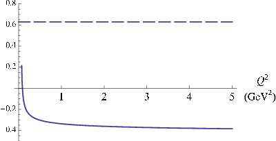 |
Most of the work towards a determination of has been done by the LHP [54] and QCDSF [70] collaborations. This year, we have seen an update from LHPC for their simulations using the mixed action approach (left plot, Fig. 15) and some preliminary results of a study using the DWF configurations from the RBC/UKQCD collaborations [13]. The results in the left of Fig. 15 indicate that the signs of the spin and orbital angular momentum contributions are opposite for each quark flavour. The same behaviour has been observed by QCDSF [70]. The lattice result is in strong disagreement with relativistic quark models and has led LHPC to search for scale dependence in , as suggested by [71]. As seen in the right of Fig. 15, they find that changes dramatically at small and in fact changes sign, which may help to reconcile the lattice and the quark model results, which generically are valid at a low hadronic scale GeV. Although as the authors point out, the one-loop evolution used here is not perhaps not quantitatively reliable below 1 GeV.
A potential improvement in the determination of from the lattice is in the extrapolation that is required from the simulated points at to the required point . As seen in Sec. 2.2, this can be achieved through the use of twisted boundary conditions, which is currently being explored by the QCDSF collaboration [25]. This may become particularly important at light quark masses when the data becomes noisier, and hence the extrapolation is poorly constrained.
5.2 Spin Asymmetries
In the past couple of years, lattice calculations of the moments of GPDs have provided facinating insights into how quarks are spatially distributed inside the nucleon [72] and pion [73]. Of particular interest is the strong correlation between the transverse spin and coordinate degrees of freedom [74], providing evidence for a sizeable Boer-Mulders function, [75].
Recently, there has been an attempt to determine on the lattice (moments of) the Transverse Momentum Dependent PDFs (TMDPDFs), e.g. , which are important in semi-inclusive DIS (SIDIS). In order to obtain information on the dependence of these functions on the transverse momentum, , of the quarks inside a hadron, it is necessary to consider matrix elements , where the quark fields are separated by a distance, , and is a Wilson line (to infinity and back). Of course, this is not possible on the lattice so instead one is required to consider a path of finite total length separating the quark and anti-quark in the operator, as illustrated in Fig. 3a of [76].
The matrix element is then obtained from from
| (14) |
Choosing to be gives access to , while gives . The -dependence of these functions is fitted with a double Gaussian. Moments of the TMDPDFs are then obtained via a Fourier transform
| (15) |
and similarly for which is obtained from .

Information on the correlation between the intrinsic quark transverse momentum and the transverse polarisation of the nucleon can then be obtained by considering the combination
| (16) |
which is shown in Fig. 16 for a longitudinally polarised -quark inside a nucleon that is transversly polarised in along the -axis, . We clearly see that the distribution is distorted along the -axis.
6 Distribution Amplitudes
Distribution amplitudes (DAs) describe the momentum-fraction distribution of partons at zero transverse separation in a particular Fock state, with a fixed number of constituents. They are essential for the determination of the hard contributions to exclusive processes, but being universal hadronic properties, are process independent. Hence, they are important for calculations of form factors at large , B-decays, and can be related to the Bethe-Salpeter wave function.
DAs are defined as non-local matrix elements on the light cone, e.g. the leading twist pion DA
| (17) |
Results for moments of the light pseudoscalar meson distribution amplitudes have been presented by QCDSF [77] and UKQCD/RBC [78] in the last couple of years. Here we will focus on some recent results for vector mesons and the nucleon.
6.1 Vector Mesons
For spin-1 mesons, there are two DA’s, , as opposed to a single DA for spin-0 mesons. The lowest moments of are obtained from the local matrix elements
| (18) | |||||
| (19) |
where and are the mass and decay constant, respectively, of the the vector meson, , and is a polarisation vector. The moments, are extracted by constructing ratios of lattice two-point functions [79, 80] and the bare lattice results are then renormalised.


In Fig. 17 we see some preliminary results from the RBC/UKQCD collaborations for and calculated with DWF configurations with 4 values of the light quark mass and 2 volumes [80]. The results indicate that there are no clear signs of finite volume effects. After renormalising perturbatively (although in [80] they also presented a status report on their nonperturbative renormalisation programme and the results should be finalised soon) to the scheme at , they find
| (20) |
which compare well with the preliminary results from QCDSF [79] , . These results show the -breaking effects in the DAs in a similar way to that observed for the DAs in [77, 78].
6.2 Nucleon
For the proton, there are three distribution amplitudes, . In a similar way to the case of mesons above, their moments () can be obtained from hadron-to-vacuum matrix elements of local operators [81]. It is useful to construct the combination, . In the asymptotic limit, and we have , , , hence it is useful to look for asymmetries, such as .


QCDSF have calculated first two moments [82] using an improved constrained analysis which considers ratios of correlators [82] together with nonperturbative renormalisation of the appropriate 3-quark operators [83]. By considering the difference between two such ratio, as shown in Fig. 18, the asymmetry is pronounced and increases as one approaches the chiral limit.
These asymmetries are visualised in Fig. 18, where the lattice moments have been used in a polynomial expansion of the full nucleon DA. Here refer to momentum fractions of the three quarks in the proton and the asymmetries indicate that the -quark with spin aligned with proton spin has largest momentum fraction (). Interestingly, the asymmetries are less pronounced than for QCD sum rules [84] and other phenomenological determinations [85].
7 Strange Quarks in the Proton
The determination of the strange quark content of the nucleon offers a unique opportunity to obtain information on the role of hidden flavour in the structure of the nucleon. Since the nucleon has no net strangeness, the strangeness contribution to the total charge of the nucleon must be zero, i.e. . However, there is no such simple constraint on either the sign or magnitude of the strangeness contribution to the magnetic moment, . Additionally, the strangeness charge radius may also be non-zero. While the latest experimental results [86] suggest that the strange form factors of the proton are consistent with zero, forthcoming experiments at JLab and Mainz will further clarify this picture. Additionally, the strangeness contribution to the total spin of the nucleon is poorly determined. Hence there is an opportunity for lattice simulations to make an important contribution to the current understanding of the role of strange quarks in the nucleon.
7.1 Indirect strangeness
An indirect method for determining the electromagnetic strangeness form factors has been proposed over the last couple of years by the Adelaide group [87]. By combining charge symmetry constraints with chiral extrapolation techniques, based on finite-range-regularisation [88], and low-mass quenched-QCD simulations of the individual quark contributions to the charge radii and magnetic moments of the nucleon octet, precise estimates of the proton’s strange electric charge radius and magnetic moment were obtained.
Recently, Lin & Orginos [27] have followed this procedure using results from a mixed action simulation (DWF valence on Asqtad sea) with pion masses in the range MeV. Their findings for the individual quark contributions to the charge radii of the nucleon octet indicate that the contribution from the heavier strange quark is smaller than those from the light quarks (Fig 20), in agreement with quenched results [41].
After taking these mixed action results and following the Adelaide method, Lin & Orginos find at
| (21) |
which is in excellent agreement with earlier findings [87] and recent JLab experiments [86].


7.2 Direct strangeness and other disconnected
Direct lattice calculations of the strangeness content are computationally demanding and are renowned for suffering from large statistical noise. Recent advances in computing power combined with technical innovations, such as all-to-all propagators [89], have led to a renewed interest in direct determinations of disconnected quantities, such as strangeness in the nucleon. This year we have seen the progress being made in this area from several groups using a variety of different methods.
The QCD collaboration [90, 59] have started a simulation to determine the gluonic and strange quark momentum fractions of the nucleon, , and the strangeness magnetic moment using dynamical clover configurations from the CP-PACS/JLQCD collaborations. They use stochastic noise sources combined with an unbiased subtraction from the hopping parameter expansion (HPE) [91], and multiple (up to 32) sources. By summing over the operator insertion times, they can then fit to the slope, as shown in Fig. 20. Their preliminary findings suggest that the strange-to-light momentum fraction ratio, , which is slightly larger than the CTEQ value, . Additionally, is studied using the overlap operator to construct [92] in quenched QCD; since ultraviolet fluctuations are expected to be suppressed due to the exponentially local nature of the overlap operator. For , a signal is obtained with accuracy, however renormalisation is required.
Another group that is making substantial progress is the Boston group [93]. They are using stochastic sources with maximum dilution with Wilson fermions and MeV. By using vacuum-subtracted currents, e.g. , they fit the three-point function directly using input from the two-point functions to calculate . They find that they are able to determine with 30% errors and their result for is consistent with zero. From the scalar form factor, they obtain the result .
There was an update [94] on work outlined in [95] to calculate and using various noise reduction techniques such as HPE, truncation solver method, truncated eigenmode approach and dilution so that the stochastic source is only defined on a single timeslice. They find a reduction in the stochastic variance at fixed cost of around 25-30. Disconnected loops are currently being calculated using Wilson propagators on a staggered sea for three valence quark masses and two sea quark masses, with plans to move on to a full simulation in the near future.
7.2.1 Scalar Form Factor
An analysis of the chiral behaviour of the scalar radius of the pion, , can lead to a determination of the LEC and it is expected to have an enhanced chiral logarithm as compared to the vector radius discussed in Sec. 2.5. Hence it is a good place to search for chiral nonanalytic behaviour in the chiral regime. However, such a calculation would need to take into account of the disconnected contribution to the form factor, and as a result it has received little attention to date.
As mentioned in Sec. 2.5, the JLQCD collaboration are computing all-to-all propagators on their overlap configurations [37]. These all-to-all propagators allow them to compute the scalar form factor of the pion, including the contributions coming from disconnected diagrams.
From the slope of this form factor, they calculate the scalar radius of the pion, , which is shown in Fig. 22 as a function of . Also shown in the plot is the result of a combined NNLO ChPT fit to , and (see Sec. 2.5), where we can clearly see the predicted chiral curvature at light quark masses. It will be interesting to see if this can be confirmed as results become available at masses below 300 MeV. After extrapolating to the physical pion mass, they find , in agreement with experiment.


8 Background Field & Polarizabilities
All of the results presented in the previous sections have been obtained using sequential source methods, where a current with a particular momentum is inserted into one of the quark propagators used to construct the hadron. Static quantities are then obtained from a fit to the momentum transfer, , dependence of the resulting form factors. An alternative method is to consider lattice simulations in the presence of constant electric, , and magnetic, , fields, and by studying the energy shifts in a hadron as a function of the field strength, it is possible to extract not only magnetic moments, but also electric and magnetic polarisabilities, and .
On a finite volume, discontinuities can occur as the quark crosses the boundary of the lattice unless the fields are quantised as . However, this means that for the volumes being used in current lattice simulations, the applied fields are so large that nonlinearities can arise (and dominate) in the -dependence of the masses and possible distortions in the particles themselves.
Aubin et al. [96] studied the finite volume effects of the magnetic moment of the baryon. They perform a test with quenched lattices for two different spatial volumes ( and ), they implement a “patch” to the field by adding the -link modification if , resulting a field that is quantised in units of . They find that when using unpatched data with , large finite size effects are seen on the small volume. However, after patching, so long as simulations are performed close to , reliable results are obtained, even on the small volume.
Having justified their method, they then proceeded to use flavours of stout-smeared clover fermions on anisotropic lattices with two spatial volumes and patched magnetic fields. One light quark propagator ( MeV) and one strange quark propagator to obtain results for the magnetic moments of and . Results for and are consistent with experiment, with the accuracy of comparable to experiment.
Tiburzi et al. [97] calculated for both neutral and charge hadrons using clover fermions on DWF sea as a test run, with valence DWF to follow. They also showed the benefit of patching, although here it is referred to as “including transverse links”, by showing that it is possible to remove “spikes” in, e.g. the pion’s effective mass, by including links such as mentioned above. The electric polarisability, , of hadrons are then determined by examining the quadratic dependence of the energy as a function of field strength, as in Fig. 22.
For charged hadrons, one must also take into account the sum of the Born couplings to the particles total charge, leading to a modification of the time-dependence of the particles two-point function. As a result, for charged hadrons are extracted from the exponential time behaviour of the two-point functions by fitting them with . While errors obtained in this initial study are fairly large, a couple of particularly interesting results are the ratio , which is found to be in good agreement with expectations from one-loop chiral perturbation theory, i.e. it scales as , and of and which are found to be negative. For the proton and neutron, they find and .
Alexandrou [98] showed that an earlier calculation of [99] can be improved by simulating with an exponential background electric field rather than the linear field used in [99].
Finally, in [100] we saw some preliminary results for on clover configurations from the CP-PACS collaboration with three lattice spacings but constant physical volume, and quark masses in the range .
9 Conclusion & Outlook
Due to recent computer and algorithmic improvements, lattice calculations of hadronic quantities are now becoming available at pion masses as low as MeV, and it is not unreasonable to expect that soon simulations will be performed close to the physical pion mass. However, as we have seen in, e.g. , finite size effects (FSE) are starting to become a serious issue. As a result, many groups are now planning future simulations on volumes as big as , in order to minimise these effects, although corrections from ChPT will still probably need to be taken into account.
This year we have seen an impressive amount of progress in many different hadronic quantities, providing fascinating insights into the structure of hadrons. From the slope of the electromagnetic form factors, charge radii are now being computed for hadrons such as in a region where we expect to see dramatic chiral curvature towards the physical point. However, as these radii are an indication of the size of a hadron, as mentioned earlier, FSE need to be considered carefully.
The scaling of hadronic form factors is now receiving an increasing amount of attention. In particular, twisted boundary conditions are providing access to small , but there also is work underway to attempt to probe the large region (¿ 4 GeV2). The small region is also an interesting place to study the Dirac and Sachs electric form factors of the neutron. The results that are now becoming available at small are not only able to help constrain static quantities such as charge radii and magnetic/quadrupole moments, but also the value of the generalised form factor , which at provides the value of the anomalous gravitomagnetic moment, which is important in Ji’s angular momentum sum rule.
Lattice calculations of moments of generalised parton distributions are providing insights into the different quark contributions to the nucleon’s spin and angular momentum, and current results indicate . These moments are also providing evidence for non-trivial transverse spin densities in the pion and nucleon.
Simulations with zero momentum transfer lead to moments of ordinary parton distribution functions, and include phenomenologically interesting quantities such as and . Here, FSE appear to playing an important role in the extraction of these quantities, especially for where we have seen FSE lowering the lattice results. While there appears to be a slight tension between the renormalisation of some of the lattice results for , the overall pattern seems to indicate that we may now at last be entering the region where the results may start to “bend down” towards the phenomenological value. Although once again, FSE are predicted to become an issue close to the physical pion mass, so care will need to be taken to ensure this encouraging behaviour continues.
Following the recent success of lattice calculations of the moments of the light pseudoscalar meson distribution amplitudes (DAs), there are now results becoming available for moments of vector meson and proton DAs. Results for the proton are providing evidence that asymmetries exist in the way the momentum of the nucleon is distributed amongst its constituent quarks, with the -quark with its spin aligned to that of the proton carrying the most momentum. The results also indicate that the symmetries are less pronounced than in QCD sum-rules.
While it is important to push these more “standard” hadronic measurements as far as we can with the new sets of dynamical configurations that are becoming available, it is also important to develop new ideas and techniques. This year we saw a number of innovative methods for accessing less well known quantities.
By considering matrix elements of operators where the quark fields are spatially separated, moments of Transverse Momentum Dependent PDFs have been computed. From these moments, it has been seen that densities of longitudinally polarised quarks in a transversely polarised nucleon are deformed.
To date, lattice calculations of hadronic quantities have neglected the contributions coming from disconnected diagrams, since these are notoriously difficult to compute. Recently, however, there has been a renewed interest in determining these disconnected contributions to investigate the strangeness and gluonic content of the nucleon and, in particular, their contributions to nucleon spin. Through the use of all-to-all propagators and various noise reduction techniques, it may now be possible to calculate some of these contributions with as small as 10% errors.
Although background field methods have been around for a long time, they have only recently received a lot of interest, since traditionally the electromagnetic fields induced on currently sized lattices were too large. However recent developments show that it is now possible to consider fields that are a factor of smaller. As a result, magnetic moments and polarisabilities can now be extracted from these simulations with much more confidence. Additionally, it has recently been shown that it is possible to extract the electric polarisabilities of charged hadrons from a lattice simulation, and preliminary results are promising.
In summary, lattice simulations of hadronic observables have received a surge of interest over the past few years, such that we are now not only in a position to confirm experimental findings from a first-principles calculation, but also to provide predictions for, and in some cases to guide, future experimental programmes.
Acknowledgements
It is a pleasure to thank C. Alexandrou, R. Babich, D. Brömmel, W. Detmold, T. Doi, Ph. Hägler, M. Gürtler, A. Jüttner, T. Kaneko, H.W. Lin, P. Moran, B. Musch, J. Negele, D. Pleiter, G. Schierholz, S. Simula, B. Tiburzi, N. Warkentin and T. Yamazaki for useful discussions and for providing me with many results and figures. I would also like to thank Ph. Hägler and R. Horsley for careful proofreading. This work is supported through the UK’s STFC Advanced Fellowship Programme under contract number PP/F009658/1.
References
- [1] M. Vanderhaeghen, PoS LAT2008 (2008) 006.
- [2] http://www.jlab.org/
- [3] K. I. Ishikawa, PoS LAT2008 (2008) 013 [arXiv:0811.1661 [hep-lat]].
- [4] K. Jansen, PoS LAT2008 (2008) 010 [arXiv:0810.5634 [hep-lat]].
- [5] K. Orginos, PoS LAT2006 (2006) 018.
- [6] P. Hägler, PoS LAT2007 (2007) 013 [arXiv:0711.0819 [hep-lat]].
- [7] J. Arrington, C. D. Roberts and J. M. Zanotti, J. Phys. G 34 (2007) S23 [arXiv:nucl-th/0611050].
- [8] M. K. Jones et al., Phys. Rev. Lett. 84 (2000) 1398 [arXiv:nucl-ex/9910005]; O. Gayou et al., Phys. Rev. C 64 (2001) 038202; O. Gayou et al., Phys. Rev. Lett. 88 (2002) 092301 [arXiv:nucl-ex/0111010].
- [9] S. J. Brodsky and G. R. Farrar, Phys. Rev. D 11 (1975) 1309; G. P. Lepage and S. J. Brodsky, Phys. Rev. D 22 (1980) 2157.
- [10] J. J. Kelly, Phys. Rev. C 70 (2004) 068202.
- [11] G. A. Miller and J. Arrington, Phys. Rev. C 78 (2008) 032201 [arXiv:0806.3977 [nucl-th]].
- [12] S. Ohta and T. Yamazaki [RBC/UKQCD] PoS LAT2008 (2008) 168 [arXiv:0810.0045 [hep-lat]].
- [13] J. D. Bratt et al., PoS LAT2008 (2008) 141 [arXiv:0810.1933 [hep-lat]].
- [14] M. Göckeler et al. [QCDSF], Phys. Rev. D 71 (2005) 034508 [arXiv:hep-lat/0303019].
- [15] C. Alexandrou et al., Phys. Rev. D 74 (2006) 034508 [arXiv:hep-lat/0605017].
- [16] S. Sasaki and T. Yamazaki, Phys. Rev. D 78 (2008) 014510 [arXiv:0709.3150 [hep-lat]].
- [17] H. W. Lin et al., Phys. Rev. D 78 (2008) 014505 [arXiv:0802.0863 [hep-lat]].
- [18] R. D. Young et al., Phys. Rev. D 71 (2005) 014001 [arXiv:hep-lat/0406001].
- [19]
- [20] C. Alexandrou et al., PoS LAT2008 (2008) 139 [arXiv:0811.0724 [hep-lat]].
- [21] C. T. Sachrajda and G. Villadoro, Phys. Lett. B 609 (2005) 73 [arXiv:hep-lat/0411033]; P. F. Bedaque and J. W. Chen, Phys. Lett. B 616 (2005) 208 [arXiv:hep-lat/0412023]; P. F. Bedaque, Phys. Lett. B 593 (2004) 82 [arXiv:nucl-th/0402051].
- [22] F. J. Jiang and B. C. Tiburzi, Phys. Rev. D 78 (2008) 037501 [arXiv:0806.4371 [hep-lat]].
- [23] B. C. Tiburzi, Phys. Lett. B 641 (2006) 342 [arXiv:hep-lat/0607019].
- [24] F. J. Jiang and B. C. Tiburzi, arXiv:0810.1495 [hep-lat].
- [25] Ph. Hägler et al., PoS LAT2008 (2008) 138.
- [26] R. G. Edwards et al. [LHPC Collaboration], PoS LAT2005 (2006) 056 [arXiv:hep-lat/0509185].
- [27] H.W. Lin et al., PoS LAT2008 (2008) 140 [arXiv:0810.5141 [hep-lat]].
- [28] H. W. Lin, S. D. Cohen, R. G. Edwards and D. G. Richards, arXiv:0803.3020 [hep-lat].
- [29] S. R. Amendolia et al. [NA7 Collaboration], Nucl. Phys. B 277 (1986) 168.
- [30] P. Brauel et al., Z. Phys. C 3 (1979) 101; H. Ackermann et al., Nucl. Phys. B 137 (1978) 294; T. Horn et al. Phys. Rev. Lett. 97 (2006) 192001 [arXiv:nucl-ex/0607005]; V. Tadevosyan et al. Phys. Rev. C 75 (2007) 055205 [arXiv:nucl-ex/0607007].
- [31] M. Foster and C. Michael [UKQCD], Phys. Rev. D 59 (1999) 074503 [arXiv:hep-lat/9810021]; C. McNeile and C. Michael [UKQCD], Phys. Rev. D 73 (2006) 074506 [arXiv:hep-lat/0603007]; P. A. Boyle et al. [UKQCD], JHEP 0808 (2008) 086 [arXiv:0804.1501 [hep-lat]].
- [32] P. A. Boyle et al. [UKQCD], JHEP 0807 (2008) 112 [arXiv:0804.3971 [hep-lat]].
- [33] J. Gasser and H. Leutwyler, Annals Phys. 158 (1984) 142.
- [34] C. Allton et al. [RBC-UKQCD Collaboration], arXiv:0804.0473 [hep-lat].
- [35] S. Simula [ETMC Collaboration], PoS LAT2007 (2007) 371 [arXiv:0710.0097 [hep-lat]].
- [36] J. Bijnens, G. Colangelo and P. Talavera, JHEP 9805 (1998) 014 [arXiv:hep-ph/9805389].
- [37] T. Kaneko et al. [JLQCD collaboration], arXiv:0810.2590 [hep-lat].
- [38] D. Brömmel et al. [QCDSF/UKQCD], Eur. Phys. J. C 51 (2007) 335 [arXiv:hep-lat/0608021]; F. D. R. Bonnet et al. [LHPC], Phys. Rev. D 72 (2005) 054506 [arXiv:hep-lat/0411028]; S. Hashimoto et al. [JLQCD], PoS LAT2005 (2006) 336 [arXiv:hep-lat/0510085].
- [39] W. M. Yao et al. [Particle Data Group], J. Phys. G 33 (2006) 1.
- [40] P. Moran et al., in preparation.
- [41] S. Boinepalli et al., Phys. Rev. D 74 (2006) 093005 [arXiv:hep-lat/0604022].
- [42] I. C. Cloet et al., Phys. Lett. B 563 (2003) 157 [arXiv:hep-lat/0302008].
- [43] J. N. Labrenz and S. R. Sharpe, Phys. Rev. D 54 (1996) 4595 [arXiv:hep-lat/9605034]; D. B. Leinweber et al., Nucl. Phys. A 737 (2004) 177 [arXiv:nucl-th/0308083].
- [44] C. Alexandrou et al., arXiv:0810.3976 [hep-lat].
- [45] M. Gürtler, PoS LAT2008 (2008) 051.
- [46] J. N. Hedditch et al., Phys. Rev. D 75 (2007) 094504 [arXiv:hep-lat/0703014].
- [47] F. X. Lee, S. Moerschbacher and W. Wilcox, arXiv:0807.4150 [hep-lat].
- [48] C. Alexandrou and G. Koutsou, arXiv:0809.2056 [hep-lat].
- [49] D. B. Leinweber et al., Phys. Rev. D 48 (1993) 2230 [arXiv:hep-lat/9212016].
- [50] C. Alexandrou et al., Phys. Rev. Lett. 94 (2005) 021601 [arXiv:hep-lat/0409122]; C. Alexandrou et al., Phys. Rev. Lett. 98 (2007) 052003 [arXiv:hep-lat/0607030]; C. Alexandrou et al., Phys. Rev. D 76 (2007) 094511.
- [51] C. Alexandrou et al., Phys. Rev. D 77 (2008) 085012 [arXiv:0710.4621 [hep-lat]].
- [52] W. Detmold et al., Phys. Rev. Lett. 87 (2001) 172001 [arXiv:hep-lat/0103006].
- [53] D. Brömmel et al., arXiv:0804.4706 [hep-lat].
- [54] Ph. Hägler et al. [LHPC], Phys. Rev. D 77 (2008) 094502 [arXiv:0705.4295 [hep-lat]].
- [55] M. Göckeler et al. [QCDSF], Phys. Rev. D 71 (2005) 114511 [arXiv:hep-ph/0410187].
- [56] K. Orginos, T. Blum and S. Ohta, Phys. Rev. D 73 (2006) 094503 [arXiv:hep-lat/0505024].
- [57] W. Detmold and C. J. D. Lin, Phys. Rev. D 71 (2005) 054510 [arXiv:hep-lat/0501007].
- [58] D. Mankame, T. Doi, T. Draper, K. F. Liu and T. Streuer, arXiv:0810.3241 [hep-lat].
- [59] M. Deka et al., arXiv:0811.1779 [hep-ph].
- [60] S. Capitani et al., Nucl. Phys. Proc. Suppl. 73 (1999) 288 [arXiv:hep-lat/9809171]; W. Detmold and C. J. D. Lin, Phys. Rev. D 73 (2006) 014501 [arXiv:hep-lat/0507007]; W. Bietenholz et al., PoS LAT2007 (2007) 159 [arXiv:0712.3772 [hep-lat]].
- [61] W. Bietenholz et al., arXiv:0808.3637 [hep-lat].
- [62] A. Ali Khan et al., Phys. Rev. D 74 (2006) 094508 [arXiv:hep-lat/0603028].
- [63] R. G. Edwards et al. [LHPC], Phys. Rev. Lett. 96 (2006) 052001 [arXiv:hep-lat/0510062].
- [64] T. Yamazaki et al. [RBC/UKQCD], Phys. Rev. Lett. 100 (2008) 171602 [arXiv:0801.4016 [hep-lat]].
- [65] R. Baron et al., PoS LAT2008 (2008) 162.
- [66] H. W. Lin and K. Orginos, arXiv:0712.1214 [hep-lat].
- [67] T. T. Takahashi and T. Kunihiro, Phys. Rev. D 78 (2008) 011503 [arXiv:0801.4707 [hep-lat]].
- [68] M. Göckeler et al. [QCDSF], Phys. Rev. Lett. 92 (2004) 042002 [arXiv:hep-ph/0304249].
- [69] X. D. Ji, Phys. Rev. Lett. 78 (1997) 610 [arXiv:hep-ph/9603249].
- [70] D. Brömmel et al. [QCDSF/UKQCD], PoS LAT2007 (2007) 158 [arXiv:0710.1534 [hep-lat]].
- [71] A. W. Thomas, Phys. Rev. Lett. 101 (2008) 102003 [arXiv:0803.2775 [hep-ph]].
- [72] M. Göckeler et al. [QCDSF], Phys. Rev. Lett. 98 (2007) 222001 [arXiv:hep-lat/0612032].
- [73] D. Brömmel et al. [QCDSF], Phys. Rev. Lett. 101 (2008) 122001 [arXiv:0708.2249 [hep-lat]].
- [74] M. Diehl and Ph. Hägler, Eur. Phys. J. C 44 (2005) 87 [arXiv:hep-ph/0504175]; M. Burkardt, Phys. Rev. D 72 (2005) 094020 [arXiv:hep-ph/0505189]; S. Meissner, A. Metz and K. Goeke, Phys. Rev. D 76 (2007) 034002 [arXiv:hep-ph/0703176].
- [75] D. Boer and P. J. Mulders, Phys. Rev. D 57 (1998) 5780 [arXiv:hep-ph/9711485].
- [76] B. U. Musch et al., [LHPC], PoS LAT2007 (2007) 155 [arXiv:0710.4423 [hep-lat]]; PoS LAT2008 (2008) 166 [arXiv:0811.1536 [hep-lat]].
- [77] V. M. Braun et al., Phys. Rev. D 74 (2006) 074501 [arXiv:hep-lat/0606012].
- [78] P. A. Boyle et al., [UKQCD], Phys. Lett. B 641 (2006) 67 [arXiv:hep-lat/0607018]; M. A. Donnellan et al. [UKQCD], PoS LAT2007 (2007) 369 [arXiv:0710.0869 [hep-lat]].
- [79] V. M. Braun et al. [QCDSF/UKQCD], PoS LAT2007 (2007) 144 [arXiv:0711.2174 [hep-lat]].
- [80] P. A. Boyle et al., PoS LAT2008 (2008) 165 [arXiv:0810.1669 [hep-lat]].
- [81] T. Kaltenbrunner et al., Eur. Phys. J. C 55 (2008) 387 [arXiv:0801.3932 [hep-lat]].
- [82] M. Göckeler et al., Phys. Rev. Lett. 101 (2008) 112002 [arXiv:0804.1877 [hep-lat]].
- [83] M. Göckeler et al., arXiv:0810.3762 [hep-lat].
- [84] I. D. King and C. T. Sachrajda, Nucl. Phys. B 279 (1987) 785.
- [85] J. Bolz and P. Kroll, Z. Phys. A 356 (1996) 327 [arXiv:hep-ph/9603289]; V. M. Braun, A. Lenz and M. Wittmann, Phys. Rev. D 73 (2006) 094019 [arXiv:hep-ph/0604050].
- [86] A. Acha et al. [HAPPEX collaboration], Phys. Rev. Lett. 98 (2007) 032301 [arXiv:nucl-ex/0609002].
- [87] D. B. Leinweber et al., Phys. Rev. Lett. 94 (2005) 212001 [arXiv:hep-lat/0406002]; Phys. Rev. Lett. 97 (2006) 022001 [arXiv:hep-lat/0601025].
- [88] R. D. Young, D. B. Leinweber and A. W. Thomas, Prog. Part. Nucl. Phys. 50 (2003) 399 [arXiv:hep-lat/0212031]; Phys. Rev. Lett. 92 (2004) 242002 [arXiv:hep-lat/0302020].
- [89] J. Foley et al., Comput. Phys. Commun. 172 (2005) 145 [arXiv:hep-lat/0505023].
- [90] T. Doi et al., PoS LAT2008 (2008) 163 [arXiv:0810.2482 [hep-lat]].
- [91] C. Thron, S. J. Dong, K. F. Liu and H. P. Ying, Phys. Rev. D 57 (1998) 1642 [arXiv:hep-lat/9707001].
- [92] K. F. Liu, A. Alexandru and I. Horvath, Phys. Lett. B 659 (2008) 773 [arXiv:hep-lat/0703010].
- [93] R. Babich et al., PoS LAT2008 (2008) 160.
- [94] G. Bali, S. Collins and A. Schafer, PoS LAT2008 (2008) 161 [arXiv:0811.0807 [hep-lat]].
- [95] S. Collins, G. Bali and A. Schafer, PoS LAT2007 (2007) 141 [arXiv:0709.3217 [hep-lat]].
- [96] C. Aubin, K. Orginos, V. Pascalutsa and M. Vanderhaeghen, arXiv:0809.1629 [hep-lat].
- [97] B. C. Tiburzi, arXiv:0809.1886 [hep-lat].
- [98] A. Alexandru and F. X. Lee, arXiv:0810.2833 [hep-lat].
- [99] J. C. Christensen et al., Phys. Rev. D 72 (2005) 034503 [arXiv:hep-lat/0408024].
- [100] S. Moerschbacher et al., PoS LAT2008 (2008) 148.