Finite Difference Methods for Second Order in Space, First Order in Time Hyperbolic Systems and the Linear Shifted Wave Equation as a Model Problem in Numerical Relativity
Abstract
Motivated by the problem of solving the Einstein equations, we discuss high order finite difference discretizations of first order in time, second order in space hyperbolic systems. Particular attention is paid to the case when first order derivatives that can be identified with advection terms are approximated with non-centered finite difference operators. We first derive general properties of these discrete operators, then we extend a known result on numerical stability for such systems to general order of accuracy. As an application we analyze the shifted wave equation, including the behavior of the numerical phase and group speeds at different orders of approximations. Special attention is paid to when the use of off-centered schemes improves the accuracy over the centered schemes.
1 Introduction
Numerical discretization of first order hyperbolic systems of partial differential equations (PDEs) is greatly simplified by a result for the linear constant coefficient case [1]: If the Cauchy problem is well-posed, then the semi-discrete problem (only discretizing space and leaving time continuous) is stable when spatial derivatives are discretized with a centered finite difference operator (CFDO). Furthermore, when using simple Runge-Kutta methods [2] for time integration, for sufficiently small time step the fully discrete problem is also stable.
Such a result does not hold in general for second order systems where first and second spatial derivatives appear [3]! In order to obtain a stable semi-discrete scheme, the second order system needs to have additional properties. In [3], which in the following we refer to as CHH, sufficient conditions for stability of the fully discrete problem were presented for such systems. Although these conditions are valid for general order centered discretizations, this point has not been explicitly made. One of the results of this article is to make this statement clear, by closing a technical gap related to the boundedness of the lower order terms. The main focus of our work is on a detailed analysis of the numerical properties of discretizations where some first order derivatives are approximated with off-centered finite difference operators and artificial dissipation is added to the equations. The motivation for choosing this more general situation comes from numerical relativity, where it is a common practice to off-center by one point the derivatives corresponding to the Lie advection terms. In numerical simulations of black holes using the BSSN formulation of the Einstein equations [4, 5, 6], this procedure of off-centering was found to be essential even for sixth order schemes [7]. Numerical solutions of the Einstein equations are currently quickly expanding our knowledge about the astrophysics of compact binaries (see [8, 9] for overviews on what has been achieved since the major breakthroughs in 2005 [10, 11, 12]), but a systematic understanding of the underlying numerical techniques has not yet been achieved.
The shifted scalar wave equation serves as a simple but powerful model in numerical relativity [13, 14, 15, 16, 17]. The particular case with zero shift and flat background (standard wave equation) has been extensively studied in [18]-[19] and high order discretization methods have been proposed. In Sec. 2 we introduce the shifted scalar wave equation as a first order in time, second order in space system, together with a summary of the well-posedness theory for mixed order systems. We show stability for our semi-discrete problem, independent of shift or dissipation terms, while the fully-discrete problem requires artificial dissipation if more than one point is off-centered. Restricting to flat space in one space dimension, Courant limits and numerical phase and group speeds are computed and analyzed in detail. It is shown that increasing the off-centering reduces the Courant limit. However, by increasing the order of approximation while keeping the off-centering fixed, does not necessarily generate lower Courant limits. Regarding the numerical speeds, it is shown that indeed there are cases when off-centering improves the accuracy over the centered scheme. This fact is illustrated also experimentally by the results of some simple numerical tests at the end of Section 5.
Our analysis of the wave equation relies on certain properties of finite difference operators, in particular on their behavior in Fourier space. We introduce these operators in Section 3 together with highlighting some relevant properties. Then, in Section 4 we address the stability method and follow in Section 5 with the analysis of the wave equation. Our results are summarized in Section 6.
2 The shifted wave equation and first order in time second order in space hyperbolic systems
The scalar wave equation in a -dimensional spacetime equipped with a Lorentzian metric reads
| (1) |
We assume a uniform time slicing for simplicity, , and perform a split introducing a positive definite d-metric , with and a shift vector (see e.g. [20]). The wave equation (1) then becomes
The mixed time-space derivatives lead to non-standard behavior as compared to the flat space wave equation with zero shift, and much of the material below will be devoted to their treatment.
We reduce the wave equation to a first order in time, second order in space form by introducing the variable , in analogy with the York-ADM-system [21] (and other common representations of the Einstein equations),
which transforms the wave equation into the first order in time, second order in space system in the way most common in numerical relativity:
| (2) |
Well-posedness for the Cauchy problem for the system (1) is a standard textbook result both in the original second order form and for reduction to first order symmetric hyperbolic form. In the latter form standard theorems for numerical stability apply [1]. Here we investigate the numerical stability for the first order in time, second order in space system (2), using the methods presented in [3]. In this respect, the appropriate generalization of the shifted wave equation is a linear system of PDEs with constant coefficients of the form [3]:
with , , and
Note that the state vector is split into two parts, are those variables for which only first spatial derivatives appear, while second spatial derivatives of the -variables do enter the PDE. The well-posedness of the Cauchy problem for first order in time, second order in space systems of PDEs systems has been clarified by [22, 23, 24, 25, 26]. We will here recall the presentation in CHH, where the well-posedness of such systems of PDEs is discussed in close analogy with the issue of numerical stability. It is natural to consider -periodic solutions and turn the analysis in Fourier space.
In Fourier space the evolution problem reduces to a system of ordinary differential equations (ODEs) for the Fourier coefficients. By performing a first order reduction in Fourier space, it can be shown that well-posedness is not influenced by lower differential order terms, which we can therefore drop and consider the second order principal symbol constructed as
where , , and .
It is shown in [3] that if there exists a matrix such that and a positive constant , such that (where ), then the problem is well-posed in the norms
In [3] an analysis of numerical stability was performed in analogy with the proof of well-posedness as we have sketched it, and which we will extend to arbitrary approximation order in Section 4. But, before going into stability analysis, we need to discuss some general properties of finite difference operators.
3 Finite Difference Operators
3.1 Construction and properties in one dimension
Consider a mesh of equidistant points , with and representing the grid spacing. Corresponding to the continuum vector function we associate the grid vector function by and .
Using consecutive points, we want to construct the finite difference operator corresponding to the -derivative. Let be the offset of these points from symmetry with respect to the center, ( for CFDO) and the direction of off-centering ( for off-centering to the right, for off-centering to the left).11 1 Though one can simplify the notation by dropping and considering , it will later turn out useful to separate the sign of and its absolute value. Then the finite difference operator to be constructed will be denoted . It is a linear combination of shift operators of the form:
| (6) |
where be the shift operator by points, . The weights can be expressed as the coefficients of in the Taylor expansion of the function
around the point up to the order (see appendix A for the proof). Using this procedure, one can deduce explicit expressions for the finite difference operators corresponding to the first and second derivative (the relations (74) from appendix A).
These expressions are fairly complicated, but they can be written in a more convenient form if we make use of the elementary finite difference operators:
| (7) |
Note that the operators and are dimensionless.
Then, a direct but lengthy calculation starting from the definitions (74) leads us to the following expressions for , , the rest and :
| (8) |
where
| (9) |
Notice that the coefficients and do not depend on , while , do depend on and .
The leading order truncation error of order is defined as
A direct calculation yields
It is well known that the centered FDO has the smallest leading order truncation error, for (see also table 1).
| n=1 | n=2 | n=3 | n=4 | |
|---|---|---|---|---|
| s=0 | ||||
| s=1 |
3.2 Fourier representation of difference operators
We assume a finite grid defined by a set of points,
| (10) |
and consider periodic grid functions , decomposed as
| (11) |
where
| (12) | |||||
The set represents the set of discrete wave numbers, and in the space of periodic grid functions the set forms a orthonormal basis with respect to the scalar product and the associated norm
| (16) |
with . The quantities represent the discrete Fourier coefficients. The scalar product satisfies the Parseval relation:
| (17) |
Let with
| (18) |
Now apply the shift operator on a basis vector . This leads to
The function represents the discrete Fourier symbol of the shift operator. For any discrete operator the Fourier symbol is defined by
and for a general finite difference operator the symbol is
| (19) |
For the elementary discrete operators (7) we obtain
and it is useful to note that .
The symbols for the first and second order derivative operators are straightforwardly computed using (8),
| (20) |
where we define
| (21) |
In the following we list a series of particularly relevant properties of the Fourier symbols, further properties are given in appendix C.
First note that the quantities and are positive, and even more, from (21) it is easy to check that the following inequalities hold:
| (22) | |||
| (23) | |||
| (24) |
The real part of the Fourier symbol of the first derivative is an even function of the frequency , while the imaginary part is an odd function. The real part of the Fourier symbol of the first derivative also
- •
vanishes for centered operators (),
- •
keeps the same sign for all frequencies, in case the operator is one-point off-centered (),
- •
changes sign for off-centering by more than one point ().
The derivatives with respect to of the Fourier functions satisfy:
| (25) | |||||
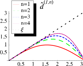
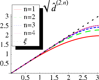
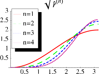
In the following we show some plots to illustrate how the errors of the Fourier symbols scale with the order of approximation and off-centering. The error is defined in respect to the continuum limit, i.e., for .
Figure 1 shows the Fourier symbols and as functions of the frequency for different orders of accuracy. For increasing approximation order, the second derivative becomes more accurate for all frequencies, while the first derivative does not converge to the continuum limit for the highest frequency in the grid, where the symbol is zero. The -frequency will not be captured also by the off-centered discrete operators associated with the first derivative. In addition, for them, the error scales with the order only at small frequencies.
Figure 2 shows the scaling of the error for with the off-centering at fixed order of approximation. In the region of small frequencies, off-centering increases the error. At larger frequencies this behavior changes. For each , there are exactly frequencies in where the error cancels. However, for there are large intervals where the error overcomes by far the error when . For we observe that while at small frequencies, the error is slightly larger than for , for each order , there is a frequency, , beyond which the error is smaller than for the case . This frequency can be computed numerically, e.g. , , , .


3.3 Generalization to -dimensions
In this work we will use the common straightforward generalization of finite difference operators from one to dimensions. We extend first derivatives in a particular coordinate direction in the trivial way, and second derivative operators in the -directions are defined as
| (26) |
The Fourier symbols for the first and second derivative operators take the form
In order to simplify notation, we will also use the following convention: any function in frequencies, and possible, grid spacings, will be referred to by , and by in case it depends on all frequencies. More detailed definitions for the -dimensional case are given in appendix B.
3.4 Dissipation Operators
In order to achieve numerical stability for problems that go beyond the linear constant coefficient case, it is common practice to add artificial dissipation to the right-hand-sides of the time evolution equations. In this work we only deal with the constant coefficient problem, but in 5.2 we will also use dissipation to stabilize numerical schemes which would be unstable otherwise.
Dissipation terms are typically chosen to converge away fast enough so as not to change the convergence order of the scheme. Here we use the Kreiss-Oliger dissipation operator of order [1] and its Fourier representation ,
| (31) |
for a accurate scheme, where the parameters regulate the strength of the dissipation. Using this form of numerical dissipation, theorems can be proved concerning the numerical stability of non-constant-coefficient hyperbolic PDEs [1]. Note that it is more common to have the dissipation parameters not depend on the direction or other parameters of the system.
4 Numerical stability for first order in time, second order in space hyperbolic systems
We now turn to the analysis of numerical stability for the system (2), following [3]. This problem is greatly simplified by adopting the method-of-lines approach where initially time is kept continuous and only space is discretized (i.e. the semi-discrete problem). Then the discrete system to be analyzed becomes
We consider periodic grid functions in each direction, and Fourier transform the system as discussed in appendix B. Then a first order reduction is performed by introducing the variable ,
| (35) |
where is the Fourier symbol of the forward finite difference operator in the -direction, . The case (which corresponds to zero frequencies in all directions) does not play any role in the stability analysis22 2 the zero frequency vector corresponds to a term constant in space., so we define and assume .
By (35) we obtain the following system of ODEs
Using the theorem 5.1.2 of [1] CHH show that the terms which correspond to the continuum lower order terms can be dropped from without affecting the stability analysis if
| (40) |
are bounded for all frequencies . In the relations (40), represents the time step. We will show in lemma 4.1 that this is indeed the case for any order of accuracy .
Having proved this, the rest of the discussion in CHH applies. The problem now reduces to the analysis of a first order system with the principal part:
For this type of system, sufficient conditions for stability have been deduced in [1]. These conditions have been exploited in CHH to analyze the stability of the second order system. By introducing the so-called second-order principal symbol of the semi-discrete system,
| (44) |
and assuming that the time integration is done using one-step explicit schemes, CHH show that the following conditions are sufficient for stability:
Condition 1: There exists a hermitian matrix such that
| (45) |
for some positive constant .
Condition 2: The eigenvalues of have non-positive real parts and
| (46) |
where is the maximum spectral radius of and is a constant specific to the time integrator.
Remarks:
- •
- •
The semi-discrete problem is stable also in the norm defined by:
(48) This norm is conserved by the principal symbol of the evolution system, .
- •
The constant in (46) denotes the radius of local stability on the imaginary axis () in case the eigenvalues of are purely imaginary, and the radius of local stability (), otherwise. 33 3 for the classical fourth order Runge-Kutta, and .
- •
In case all the grid spacings are equal, , and we introduce the Courant factor , then the relation (46) provides the Courant limit:
(49) - •
If the right hand side of the system (4) is modified by adding artificial dissipation (using the operator defined in (31)) and/or by adding shift advection terms of the form (where is the non-centered FDO in the -direction constructed from (8)), these modifications only have effect on the diagonal entries of the principal part. The new system will have different eigenvalues than but the same set of eigenvectors. The symmetrizer will not depend on the way we discretize the advection terms, nor on the dissipation operator. The stability Conditions 1-2 remain valid if
(50) are bounded and this will be shown below together with the boundedness of the terms (40).
Lemma 4.1
The following quantities are bounded for all frequencies .
| (51) |
Making use of the relations (3.3) and (31), the proof reduces to showing the boundedness of
From the relations (21) we observe that each of these quantities can be written formally as a product , with a continuous and bounded function in . Since is bounded for all , but not all zero in the same time, we obtain the desired result.
5 Application: Scalar Wave Equation
5.1 Semi-discrete Problem
The system (2) is discretized assuming, for simplicity, that the grid spacings are equal (). The case for some directions and does not introduce further complications in the following analysis.
We construct the semi-discrete system corresponding to (2) by:
| (52) |
This way of discretizing the first order derivative terms, which correspond to advection along the shift vector , with off-centered derivatives has become customary in numerical relativity (see e.g. [27, 28, 7]).
We define the shorthand quantity as
Then the discrete symbol, the diagonalizing matrix and the eigenvalues can be written as
| (53) |
| (54) |
Because , according to (21), and the matrix is positive definite, the quantity is real and with equality only when all are zero. Thus
is a symmetrizer for the system (52). We observe that the symmetrizer does not depend on the diagonal entries of the symbol , e.g. does not depend on the way we advect the shift terms.
We still have to prove that there exists a constant such that
| (55) |
The positivity of the matrix implies the existence of a constant such that
| (56) |
Furthermore, because there also exists a constant such that
| (57) |
Using (56) and the inequalities (24) we obtain
On the other hand, by (57) and again (24) we have that
We chose and obtain the relation
(55).
The conserved discrete quantity in physical space associated to , i.e. the norm defined in (48), is
where . Having proved the existence of a symmetrizer we have proved that the semi-discrete problem is stable with respect to the norms and . Note again that the stability property does in particular not depend on how the shift terms are discretized.
5.2 Courant Limits and the Role of Dissipation
In order for the fully discrete problem to be stable we impose the non-positivity condition on the real part of the eigenvalues and restrict the Courant factor according to the inequality (49):
| (58) | |||||
| (59) |
From (54) we have
| (60) |
The relation (58) has to hold for all frequencies . Because each term in the sum (60) can be canceled individually at , the non-positivity condition has to applied for each term. The problem reduces to the study of the one-dimensional case,
| (61) |
Because is zero for , negative for and changes sign for , it is clear that the condition holds for centered and one-point upwinded () schemes and is violated in all the other cases.
However, the condition can be reestablished if appropriate artificial dissipation is added to the system. By using the Kreiss-Oliger dissipation operator (31), the condition (61) changes to
| (62) |
This imposes a lower limit on the dissipation parameter :
| (63) |
where we have denoted
| (64) |
and used the fact that is, according to (21), a sum over powers of .
In table 2 we give the formulas for for . We remark that for all , , and for all .
This means that when using one-point upwinded stencils, we can add “negative” dissipation and still obtain a stable scheme. In fact, the following situations are equivalent:
- •
Upwind one point and add dissipation with .
- •
Downwind one point and add dissipation with .
- •
Use the CFDO operator (constructed with points), and do not add dissipation, .
In any of the above three situations, the real part of the eigenvalues is zero, so if the Courant limit is small enough then we obtain stability on the imaginary axis.
| s=1 | ||
|---|---|---|
| s=2 | ||
| s=3 |
Now, coming back to the -dimensional case, it is obvious that the dissipation parameters in (31), , have to be chosen according to the value of the shift and the type of off-centering in the -direction (). It can shown that, by choosing exactly the Courant limit is maximized. However, to compute it explicitly, (as a function of shifts, order of approximation, and off-centerings) is not easy in the general case.
In the particular case of a flat -metric with zero shift, the Courant limit is easy to write down:
where is given in (24) and . In the general case, the Courant limit has to be evaluated numerically.
For the 1-D wave equation with shift with upwind discretization of the advection term and adding the minimal amount of dissipation if necessary, the limit of the Courant factor is given by


We compare the Courant limits for different orders of approximations at fixed advection stencil in Figure 3, and the Courant limit at fixed order of approximation for different advection stencils in Figure 4.
In Figure 3 we see that if , the higher the order of approximation, the lower the Courant limit. For , this is not true anymore beyond a certain value of the shift. For large shifts we observe that increasing the order of approximation, actually decreases the Courant limit.
Comparing different stencils in Figure 4, we observe that advecting more points decreases the Courant limit, and there is a significant drop in the Courant factor between and , for all orders of approximation.
5.3 Phase and Group Speeds
For the wave equation the continuum phase and group speeds are:
where and . The discrete speeds can be defined in a simillar manner from the discrete eigenvalues . This would lead to complex speeds in case of off-centered schemes which are difficult to investigate [29]. In the following, we assume that the real part of the discrete eigenvalues has been cancelled by adding appropriate artificial dissipation terms (positive or negative). Otherwise, our investigation remains valid only at small frequencies, where the damping/amplification effect introduced by the real part is dominated by the dispersion effect associated to the imaginary part of the eigenvalues. With these remarks, we define the discrete speeds by:
We also restrict attention to the one dimensional case. Because speeds interchange when changes sign, it is enough to consider only the “+” speed over the whole spectrum . Also because we will compare speeds at different orders of approximation or at different stencils, we attach the superscript (or only in case ), to the symbols representing the discrete speeds and the corresponding errors:
The continuum limits for both, phase and group speeds are for and for . We will analyze the behavior of the speed errors defined as
| (65) | |||||
| (66) |
We will also assume without restricting generality, if , then .
5.3.1 Small Frequencies
When one can show that the phase and group speed errors satisfy
Because the errors scale with ,
it is obvious that for small enough frequencies higher order
approximations will improve the phase and group errors for all the
values of the shift and for all advection stencils.
If we keep the order fixed and compare the speeds corresponding
to an off-centering by -points with the ones corresponding to
the centered scheme, , then one can easily show that the
off-centered scheme improves over the centered one
- •
the “+” numerical speeds () if is odd and is small enough
- •
the “-” numerical speeds () if is even and is small enough
where small enough means
Obs. For , the above inequality becomes .
Also notice that with increasing the above limit on decreases.
In the next subsection we will analyze the behavior
for the whole spectrum in some more detail.
5.3.2 Comparison with wave equation written in first order form
If the wave equation is written in first order form (approximating the first derivatives with the corresponding CFDO), then the eigenvalues become . For one then gets
We notice that for a given order, the second order system discretized with CFDO, has smaller phase and group errors then the first order one (for both eigenvalues), if and only if . If is not in this interval then one pair of speeds (phase and group) is better approximated by the second order system, while the other one is better approximated by the first order system.
5.3.3 Scaling of the Speed Errors with the Order of Approximation
Lemma 5.1
If , then increasing the order of approximation decreases the phase and group speed errors for all frequencies.
To prove this we make use of the relations (25) in the definitions of the speeds and obtain
Using the inequalities (22) and (23) one can easily show that and for all frequencies. The situation is illustrated in Figure 5 where we plot the speeds and versus .


If then it is not true anymore that higher order approximations improve the numerical speeds for all frequencies (not even for the case of using CFDO). Though one can go into details and determine the regions in the spectrum where the scaling with order fails, we restrict ourselves to illustrating this situation by plotting the numerical speeds versus frequency at a particular value of the shift. In Figure 6 we show the numerical speeds at different orders of approximation with the same advection stencil when .


5.3.4 Scaling of the Speed Errors with Off-centering
The next question we want to answer is what happens with the numerical speed errors, if we keep the order of approximation fixed and vary the off-centering of the first derivative. For example, we illustrate this situation in Figure 7, when . As one can see already in these plots, although we know that off-centering increases the error of the finite difference operator, it is not necessary that the numerical speeds will follow the same pattern. E.g. for this value of the shift, the ”+” speed seems more accurate with than with for all the spectrum.


In the following we will determine the regions in the -plane where off-centering improves the numerical speed errors over the centered scheme.
Phase Speeds
Imposing and using the definition (65) yields the inequality
| (67) |
where
| (68) |
We have but can change
sign over the spectrum.
The inequality (67) holds at a given frequency ,
if and
or and .
In general, the regions in plane where
at fixed order of approximation,
off-centering by points improves the accuracy of the phase speed,
are difficult to determine analytically and we restrict ourselves
to a numerical evaluation (Figure 8).
What we see in the plots is that if is odd (even)
then for sufficiently small ,
the “+” (“-”) speed has smaller error
compared with the case of CFDO in some intervals of the spectrum
that include the small frequency range.
However these regions become narrower with increasing the off-centering,
such that for we have the strongest effect.
We analyze this case in more detail below.
If , the functions and ,
defined in (68) become
| (69) |
We have
and .
Then the inequality holds
- •
for if or ,
- •
for if .
The limits of in and are
It can be shown that the equation has at most one solution in each of the branches and , that we will denote by . It turns out that holds if
- •
and ,
- •
and ,
- •
and .
At a given order of approximation, , for sufficiently small the “+” speed has smaller error in the case when we advect one point than in the case when we use CFDO, for all frequencies , but the “-” speed will have larger error, at least for small and mid frequencies.
If then for both speeds, in the regime of small frequencies, the CFDO give less error than one-point advected scheme, while for mid and high frequencies the situation reverses. The interval of small frequencies where CFDO are better than advected scheme shrinks with increasing the order of approximation.


Group Speeds
Imposing and using the definition (66) yields the inequality
where
| (70) |
and and are given by (68).
It is easy to see that .
However the signs of are more difficult
to determine.
As in the case of phase speeds analysis, we determine graphically
(see Figure 9) the regions in plane where
at fixed order of approximation,
off-centering by points improves the accuracy of the group speed.
We see the same qualitative behavior as for the phase speeds,
in the sense that for sufficiently small ,
the “+” (“-”) speed has smaller error
compared with the case of CFDO at least at small frequencies,
and off-centering decreases the extent of these regions
in -space.
In case , the relations (70) become
| (71) |
By analyzing the monotony of these functions using the properties from 3.2, the following result can be formulated:
At a given order of approximation , for sufficiently small , the “+” group speed has smaller error in the case when we advect one point than in the case when we use CFDO for all frequencies , (in the case of phase speed this was the whole range !), but the “-” speed will have larger error, at least for small and mid frequencies.
If then for both speeds, in the regime of small frequencies, the CFDO give less error than one-point advected scheme, while for mid and high frequencies, the situation reverses. The interval of small frequencies where CFDO are better than advected scheme narrows with increasing the order of approximation.


5.3.5 Centered versus One-Point Upwinded Scheme, Numerically


In 5.3.4 we showed that when the numerical “+” speeds are better approximated with one-point off-centered schemes than with centered schemes at least up to very high frequencies in the grid. In this section we show some simple numerical tests to illustrate this fact. We chose -periodic initial data:
| (72) |
The parameter sets the amplitude of the “” components,
When the signal is purely “left” (“right”) going and when , the signal is equally distributed between both modes.
We choose a grid with points and resolution , the width of the grid is . Also we chose , and we integrate the wave equation using fourth order FDOs for space derivatives and the fourth order Runge-Kutta as time integrator.
We let and for each value of we look at the errors for the main variables when (see Figure 10). The numerical results show that, indeed, when the signal is “left” going, the upwinded scheme has less error than the centered scheme, while when the signal is going “right”, the centered scheme is to be preferred.
6 Conclusions
In this paper we have investigated several aspects related to the discretization of the initial value problem for first order in time and second order in space systems of differential equations, using high order finite difference operators. Special attention has been paid to the situation when some of the first derivatives are approximated with off-centered discrete operators as is customary for treating black hole spacetimes in numerical relativity. Our investigation has been divided into three parts: (a) We started with an analysis of certain properties of the finite difference operators (Section 3). (b) Using these properties we have extended the validity of an existing stability method (Section 4). (c) We analyzed the stability and the numerical speeds in the case of the scalar wave equation (Section 5).
In the following we will give a brief overview of the results.
(a) Analysis of first and second order discrete derivative operators
A set of mathematical properties have been deduced for the Fourier symbols associated with the second order centered and first order (not necessarily centered) discrete derivatives. They are in the form of inequalities, recursive and differential relations for the Fourier symbols at different orders of approximation or at different off-centerings. Here we mention two of them:
While first derivatives do not converge in the limit at the maximum grid frequency (), second derivatives do converge at all frequencies (that is the highest frequency in the grid will not be captured by the first order derivative, regardless of the order of approximation or the off-centering, while the second centered derivative can “see” it and approximates it better with increasing order).
For first order derivatives, increasing the off-centering () at a fixed order of approximation increases the error of the derivative at small frequencies. At larger frequencies this behavior changes. E.g., for , beyond a certain frequency , the error is smaller than for the case . As a consequence, off-centering of the first order derivative in the case of the advection equation, increases the error at small frequencies, while at high frequencies, this situation can reverse.
(b) Generalization of a stability analysis method
In [3], necessary and sufficient conditions for stability have been deduced assuming that (2) is discretized using 2nd or 4th order CFDOs and integrated in time using a time integrator locally stable on the imaginary axis. The validity of this stability method is extended here to -order spatial accuracy, including also the case where some derivatives are approximated with non-centered FDOs and dissipation is added to the system. It is pointed out that neither adding artificial dissipation nor shift advection terms affects the eigenvectors of the discrete symmetrizer, and thus the conditions for semi-discrete numerical stability. The Courant limit will of course be affected in general.
(c) Application: Scalar Shifted Wave Equation
The stability method presented in Section 4 is applied to the case of the wave equation on a curved background in dimensions.
In the case of 1-D shifted wave equation in flat spacetime, the Courant limits and the numerical speeds have been analyzed in detail in respect to the order of approximation and off-centering of the first derivative.
- •
Courant limits
Off-centerings by more than one point require dissipation for stability. In these cases, the minimal Kreiss-Oliger dissipation needed for stability has been computed and found to be proportional to the shift . For centered schemes, higher order approximations have lower Courant limits. Interestingly, this does not hold for off-centered schemes (when adding just dissipation to be in the local stability regime) — for large enough shift, the Courant limit is actually larger for higher order schemes. Off-centering generally reduces the Courant limit drastically, except for at least fourth order accurate schemes, when only one-point off-centering is used: for higher than fourth order schemes one-point off-centering only leads to a minor reduction of the CFL factor.
- •
Numerical speeds
Without shift, higher order approximations always result in more accurate numerical speeds, with nonzero shift this is not generally true at higher frequencies.
Although the truncation error for the first order derivative increases with the off-centering, the mixing with the second order discrete derivative in the scheme, causes upwinded stencils to give a higher overall accuracy in some situations.
More precisely, it is shown that advecting shift terms by an odd (even) number of points reduces the errors of the “” (“”) numerical speeds in some intervals of the spectrum that include the small frequency range, if the shift is not too large. The extent of the regions in the (frequency, shift)-parameter space where this improvement appears, decreases with off-centering, in such a way that for one gets the strongest effect.
Thus, at a given order , if the shift satisfies , then off-centering by one point has in comparison with the centered scheme, better “” phase speed error for all frequencies, and better “” group speed error for all frequencies up to a very high frequency in the grid, .
If the wave equation is written in first order form and discretized using CFDO, then for a given order of approximation, the second order system discretized also with CFDO has smaller phase and group errors than the first order one, if . If is not in this interval then one pair of speeds (phase and group) is better approximated by the second order system, while the other one is better approximated by the first order system.
A detailed understanding of finite difference algorithms for first order in time, second order in space systems, in particular as applied to the Einstein equations, will require significant further work. Already for the shifted wave equation, it will be interesting to study the errors in the multidimensional case, e.g. when the wave propagates in a direction that is not aligned with the grid. A similar analysis for the full Einstein equations will require a substantial use of computer algebra methods. We also point out that for the Einstein equations much of the complications come from the nonlinear source terms, which are beyond the scope of our present analysis.
Acknowledgments
M. Chirvasa would like to thank Bela Szilagyi for inspiring discussions at the early stages of this work, and we thank Jeffrey Winicour and Gerhard Zumbusch for helpful comments on our manuscript. S. Husa has been in supported in part as a VESF fellow of the European Gravitational Observatory (EGO), by DFG grant SFB/Transregio 7 “Gravitational Wave Astronomy”, by DAAD grant D/07/13385 and grant FPA-2007-60220 from the Spanish Ministerio de Educación y Ciencia.
Appendix A Explicit Expressions for Finite Difference Operators
Explicit formulas for general finite difference operators in one dimension can be constructed in a surprisingly simple way by use of the in the following lemma.
Lemma A.1
Consider a general finite difference operator , which is written as a linear combination of shift operators of the form (6)
Then the coefficients are the coefficients of in the Taylor expansion of the function
around the point up to the order . In general, the accuracy of this operator will be .
To prove the lemma, it is enough to consider the scalar function with and the associated grid function. By applying accordingly the differential and discrete operators we get:
| (73) |
Introduce which gives . The relations (73) lead to
In the limit , . The function is now Taylor expanded around the point up to and the coefficients are identified. What remains is:
After replacing with its definition and taking the limit we obtain and the lemma is proved.
Corollary A.2
The FDOs associated with the first and second derivative are
| (74) |
where
In the relations above, is the harmonic number. Note that for .
Appendix B Finite difference operators in -dimensions
Consider a -dimensional grid defined by the set of points , where is a multiple index, and represents the grid spacing in -direction (). Corresponding to the continuum vector-function we associate the grid vector-function such that .
The shift operator by -points in the -direction, is defined by
| (75) |
A discrete operator acting in the -direction is constructed as a linear combination of the shift operators defined in (75) using the same weights as the corresponding one dimensional operator ; an operator acting in -directions is constructed as a composition of one-directional operators :
| (76) | |||||
| (77) |
In order to represent the functions in Fourier space, we consider only grid function which are periodic in each direction and limit the grid to having a finite number of points, for the direction , . We introduce
In the relations above, , and have been defined in (10), (3.2) and (18), respectively. Then, the formulas for the Fourier decomposition (11), scalar product and a norm (16) and Parseval relation (17) are valid also in -dimensions.
Appendix C Further Properties of the Fourier symbols
- 1.
Recurrence relations:
- 2.
Small frequency behavior:
- 3.
Sums
- 4.
Limits :
- 5.
The -norm defined by
is equivalent with the norm. This norm has been used to prove strong stability of the initial boundary value problem for the wave equation in [16] for the second and fourth order accuracy case.
References
- [1] B. Gustafsson, H. O. Kreiss, J. Oliger “Time dependent problems and difference methods” J.Wiley&Sons, New-York (1995).
- [2] E. Hairer, S.P. Norsett, G. Wanner,, “Solving Ordinary Differential Equations. I: Nonstiff Problems”, Springer-Verlag, Berlin, 1987
- [3] G. Calabrese, I. Hinder, S. Husa, J. Comput. Phys 218 607 (2006).
- [4] M. Shibata and T. Nakamura, Phys. Rev. D 52 (1995) 5428.
- [5] T. W. Baumgarte and S. L. Shapiro, Phys. Rev. D 59 (1999) 024007.
- [6] C. Gundlach and J. M. Martin-Garcia, Phys. Rev. D 74 (2006) 024016.
- [7] S. Husa, J. A. Gonzalez, M. Hannam, B. Brügmann and U. Sperhake, Class. Quant. Grav. 25 (2008) 105006.
- [8] F. Pretorius, arXiv:0710.1338 [gr-qc].
- [9] M. Hannam, Class. Quant. Grav. 26 (2009) 114001 [arXiv:0901.2931 [gr-qc]].
- [10] F. Pretorius, Phys. Rev. Lett. 95 (2005) 121101.
- [11] M. Campanelli, C. O. Lousto, P. Marronetti and Y. Zlochower, Phys. Rev. Lett. 96 (2006) 111101.
- [12] J. G. Baker, J. Centrella, D. I. Choi, M. Koppitz and J. van Meter, Phys. Rev. Lett. 96 (2006) 111102.
- [13] B. Szilágyi, H.-O. Kreiss, J. Winicour, Phys. Rev. D 71, 104035 (2005)
- [14] M. Babiuc, B. Szilagyi and J. Winicour, Lect. Notes Phys. 692 (2006) 251.
- [15] M. C. Babiuc, B. Szilagyi and J. Winicour, Class. Quant. Grav. 23 (2006) S319.
- [16] G. Calabrese, C. Gundlach Class. Quantum Grav. 23, S343-S367 (2006).
- [17] M. Motamed, M. Babiuc, B. Szilágyi, H-O. Kreiss, J. Winicour, Phys.Rev. D73 124008 (2006).
- [18] G. Cohen, “Higher-Order Numerical Methods for Transient Wave Equations”, Springer, (2001).
- [19] L. Anné, P. Joly and Q.H. Tran, “Construction and analysis of higher order finite” “difference schemes for the 1D wave equation”, Comput. Geosci., vol. 4, no. 3, pp. 207–249 (2000).
- [20] R. M. Wald, General Relativity, Univ. Chicago Press (1984).
- [21] J. W. York in Sources of Gravitational Radiation, Smarr, L. (ed.) (Cambridge University Press, 1979).
- [22] O. Sarbach, G. Calabrese, J. Pullin, and M. Tiglio, Phys. Rev. D 66, 064002 (2002).
- [23] G. Nagy, O. Ortiz, and O. Reula, Phys. Rev. D 70, 044012 (2004)
- [24] C. Gundlach, J.M. Martin-Garcia, Phys. Rev. D 70, 044031 (2004).
- [25] C. Gundlach, J.M. Martin-Garcia, Phys. Rev. D 70, 044032 (2004).
- [26] H. Beyer, O. Sarbach, Phys. Rev. D 70, 104004 (2004).
- [27] M. Alcubierre, B. Brügmann, Phys. Rev. D 63, 104006 (2001).
- [28] Y. Zlochower, J. G. Baker, M. Campanelli and C. O. Lousto, Phys. Rev. D 72, 024021 (2005).
- [29] L. N. Trefethen, SIAM Review, Vol. 24, No. 2, pp. 113-136, (1982).