SLAC–PUB–13498

The Standard Model of Particle Physics (SM) has been very successful in describing a wide range of elementary particles phenomena to high accuracy. A key ingredient of the model is the scalar Higgs field, responsible for electroweak symmetry breaking and for generating the masses of essentially all massive elementary particles [1, 2, 3]. Similar fields exist in extensions of the SM, such as the Minimal Supersymmetric Standard Model (MSSM). In the SM, the Higgs boson is the only particle that remains undiscovered, and its properties are determined by its mass. It is a main goal of current and future high energy physics experiments to identify the Higgs boson and explore the details of the Higgs sector. In particular, the discovery of the Higgs boson could take place at Run II of the Tevatron at Fermilab; if not there, then at the Large Hadron Collider (LHC) at CERN. Precise measurements of its properties will be one of the tasks of the proposed International Linear Collider (ILC). There is an option to use the ILC as a photon collider, by backscattering laser light off of the high energy electron beams. The high energy, highly polarized photons produced in this way can be used to study the various Higgs couplings to very high accuracy [4, 5, 6, 7, 8, 9].

The mass of the Higgs boson in the SM and MSSM has already been constrained by experiment to a range well within the reach of the aforementioned designed machines. Precision electroweak measurements have put an upper bound on the allowed values for its mass, $m_{H}\lesssim 170$ GeV at 95% confidence level in the SM [10, 11]. In the MSSM the Higgs boson mass obeys the bound $m_{H}\leq m_{Z}$ at tree level; radiative corrections increase this limit to about 135 GeV [12, 13, 14]. The mass of the Higgs boson has also been bounded from below via the Higgs-strahlung process $e^{+}e^{-}\rightarrow HZ$ at LEP2, with $m_{H}\gtrsim 114.1$ GeV in the SM and $m_{H}\gtrsim 91.0$ GeV in the MSSM [15, 16, 17, 18, 19, 20].

At a photon collider, among the two possible modes, $\gamma\gamma$ and $e\gamma$, the former is especially useful for Higgs physics. For $m_{H}<140$ GeV, the most important channel involves Higgs production via photon fusion, $\gamma\gamma\rightarrow H$, followed by the decay $H\rightarrow b\bar{b}$ [21, 22]. The advantage of this channel is that the amplitude for the continuum $\gamma\gamma\rightarrow b\bar{b}$ background to the Higgs signal is suppressed by a factor of $\mathcal{O}\left(m_{b}/\sqrt{s_{\gamma\gamma}}\right)$ when the initial-state photons are in a $J_{z}=0$ state. The production of a light SM Higgs boson through this process has been studied in a series of papers, including the radiative QCD corrections to the signal and to the backgrounds [23, 24, 25, 26, 27, 28, 29, 30, 31, 32, 33, 34, 35, 36]. The anticipated experimental uncertainty in the measurement of the partial Higgs width, $\Gamma(H\rightarrow\gamma\gamma)\times\mathrm{Br}(H\rightarrow b\bar{b})$, assuming an integrated luminosity of 80 fb^-1 in the high energy peak, is about 2% for $m_{H}<140$ GeV [37, 38, 39, 40, 41, 42, 43, 33, 34, 6].

It is important to know that no other effect can contaminate the $b\bar{b}$ signal at the 1% level. A possible concern studied in this paper is the interference between the resonant Higgs amplitude $\gamma\gamma\rightarrow H\rightarrow b\bar{b}$, and the continuum $\gamma\gamma\rightarrow b\bar{b}$ process. Similar effects have been studied previously in $gg\rightarrow H\rightarrow t\bar{t}$ at a hadron collider [44], and in $\gamma\gamma\rightarrow H\rightarrow W^{+}W^{-}$, $ZZ$ and $t\bar{t}$ at a photon collider [45, 46, 47]. These studies assumed a Higgs boson sufficiently heavy that its width was at the GeV scale due to on-shell decays to $W^{+}W^{-}$, $ZZ$ and $t\bar{t}$. In the MSSM, interference effects in $\gamma\gamma\rightarrow H\rightarrow b\bar{b}$, as well as in decays to several other final states, were taken into account, including also Sudakov resummation [48, 49]. However, explicit results separating out the interference contributions in the SM were not presented. The significance of such interference effects in CP asymmetries for various channels of MSSM Higgs production and decay at a photon collider has also been explored [50]. In the case of a light SM Higgs boson, with an MeV-scale width, the interference in $gg\rightarrow H\rightarrow\gamma\gamma$ was considered at the LHC [51]. Resonance-continuum interference effects are usually negligible for a narrow resonance, and for $m_{H}<$ 150 GeV the width $\Gamma_{H}$ is less than 17 MeV in the SM.¹¹ 1 In the MSSM, the widths of light Higgs bosons may be GeV-scale if $\tan\beta$ is large, e.g. as considered in ref. [50]. However, the $\gamma\gamma\rightarrow H\rightarrow b\bar{b}$ resonance is also rather weak, since it consists of a one-loop production amplitude. Therefore a tree-level, or even one-loop, continuum amplitude can potentially compete with it, especially since the tree-level $\mathcal{O}\left(m_{b}/\sqrt{s_{\gamma\gamma}}\right)$ suppression of the $\gamma\gamma\rightarrow b\bar{b}$ continuum amplitude is absent at one loop. In the analogous case of $gg\rightarrow H\rightarrow\gamma\gamma$, a suppression of $\sim$ 5% was found due to continuum interference [51].

In the SM, the production amplitude $\gamma\gamma\rightarrow H$ proceeds at one loop and is dominated by a $W$ boson in the loop, with some top quark contribution as well. The decay $H\rightarrow b\bar{b}$ and the continuum $\gamma\gamma\rightarrow b\bar{b}$ amplitudes proceed at tree level. For $m_{H}<160$ GeV, the Higgs boson is below the $t\bar{t}$ and $WW$ thresholds, so the resonant amplitude is predominantly real (i.e., has no absorptive part), apart from the relativistic Breit-Wigner factor. The full $\gamma\gamma\rightarrow b\bar{b}$ amplitude is a sum of resonance and continuum terms,

where $s=s_{\gamma\gamma}$ is the photon-photon invariant mass. The interference term in the cross section is given by

Since the intrinsic Higgs width $\Gamma_{H}$ is much narrower than the spread of the luminosity spectrum in $\sqrt{s}$ [9] and the experimental resolution $\delta m_{H}\sim$ 0.5 GeV [8], the observable interference effect is the integral over $s$ across the entire linewidth. Neglecting the tiny $s$-dependence of $\mathrm{Re}\left\{\mathcal{A}^{*}_{\gamma\gamma\rightarrow H}\mathcal{A}^{*}_{H\rightarrow b\bar{b}}\mathcal{A}_{\gamma\gamma\rightarrow b\bar{b}}\right\}$, the integral of the first “real” term vanishes, as it is an odd function of $s$ around $m_{H}^{2}$. The second “imaginary” term is an even function of $s$ around $m_{H}^{2}$ and therefore survives the integration. However, it requires a relative phase between the resonant and continuum amplitudes. As described above, in the SM the resonant amplitude is mainly real, apart from the Breit-Wigner factor. The tree level continuum $\gamma\gamma\rightarrow b\bar{b}$ amplitude is also real.

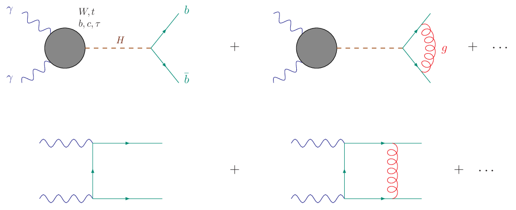
The imaginary parts of the $H\rightarrow b\bar{b}$ and $\gamma\gamma\rightarrow b\bar{b}$ amplitudes arise at one loop, when we include the exchange of a gluon between the $b$ and $\bar{b}$ quarks. These contributions are shown schematically in fig. 1. In fact, each amplitude individually has an infrared divergence from the soft-gluon exchange that builds up the Coulomb phase. However, the divergence cancels in the relative phase entering $\mathrm{Im}\left\{\mathcal{A}^{*}_{\gamma\gamma\rightarrow H}\mathcal{A}^{*}_{H\rightarrow b\bar{b}}\mathcal{A}_{\gamma\gamma\rightarrow b\bar{b}}\right\}$. Thus we are left with a finite contribution to $\delta\sigma_{\gamma\gamma\rightarrow H\rightarrow b\bar{b}}$ in eq. (2). To compute the fractional interference correction to the resonance, we divide eq. (2) for $\delta\sigma_{\gamma\gamma\rightarrow H\rightarrow b\bar{b}}$ by the square of the resonant amplitude in eq. (1). We then expand all the amplitudes in $\alpha_{s}$, obtaining

where the superscript $(l)$ denotes the number of loops ($l=1,2$) for each term in the expansion, e.g. $\mathcal{A}_{\gamma\gamma\rightarrow H}=\mathcal{A}^{\left(1\right)}_{\gamma\gamma\rightarrow H}+\mathcal{A}^{\left(2\right)}_{\gamma\gamma\rightarrow H}+\ldots$.

Taking into account that the tree amplitude $\mathcal{A}^{\mathrm{tree}}_{H\rightarrow b\bar{b}}$ has no absorptive part, we can rewrite $\delta$ as

We neglect the two-loop amplitude $\mathcal{A}^{(2)}_{\gamma\gamma\rightarrow H}$, because in the SM it is dominantly real for $m_{H}<2m_{W}$, like $\mathcal{A}^{(1)}_{\gamma\gamma\rightarrow H}$, up to small contributions from loops of lighter fermions. We also separate out the contribution from the small imaginary part of $\mathcal{A}^{\left(1\right)}_{\gamma\gamma\rightarrow H}$, obtaining the expression

The two photons in eq. (5) are taken to have identical helicity in all amplitudes, so that $J_{z}=0$ as required for interference with the production of the scalar Higgs boson.

We determine the imaginary parts of the two terms in the braces in the second line of eq. (5) by analyzing the unitarity cuts of the diagram in fig. 2. The first term, $\mathrm{Im}\Bigl\{\mathcal{A}^{\mathrm{{}^{*}tree}}_{H\rightarrow b\bar{b}}\mathcal{A}^{\left(1\right)}_{\gamma\gamma\rightarrow b\bar{b}}\Bigr\}$, comes from interpreting the $b$ quarks crossing the left cut as the actual final-state $b$ quarks, emerging at a fixed scattering angle $\theta$. The imaginary part of the tensor box integral to the right of the left cut is associated with $b$-quark rescattering; thus one integrates over the $b$ momenta crossing the right cut. The second term, $-\mathrm{Im}\Bigl\{\mathcal{A}^{\mathrm{tree}}_{\gamma\gamma\rightarrow b\bar{b}}\mathcal{A}^{{}^{*}\left(1\right)}_{H\rightarrow b\bar{b}}\Bigr\}$, comes from exchanging the roles of the left and right cuts.

We use FORM [52] for symbolic manipulations, and the decomposition of the scalar box integral into a six-dimensional scalar box plus scalar triangle integrals [53]. In the expressions below, we use the same notation as in ref. [53]; primed quantities correspond to particular tensor integrals. After cancelling the divergent parts arising from both terms (associated with the scalar triangle integral $I_{3}^{(2)}[1]$), the finite imaginary parts are given by

where

and

In the expressions above,

and

where $\theta$ is the $\gamma\gamma\rightarrow b\bar{b}$ center-of-mass scattering angle. The terms in eqs. (6) and (7) that are obtained by substituting $\cos\theta\rightarrow-\cos\theta$ (or, equivalently, $t\rightarrow 2m_{b}^{2}-m_{H}^{2}-t$) arise from a diagram like that in fig. 2, but with the two photons exchanged.

It is worth noting that the absence of bubble integrals from eq. (6) is due to a cancellation among the scalar and tensor bubble terms, and that the tensor triangle contribution in eq. (7) has been expressed in terms of the tensor triangle integral $I_{3}^{\left(2\right)\prime}$ appearing in eq. (6). After adding the terms with $\cos\theta\rightarrow-\cos\theta$, the contributions from $I_{3}^{\left(2\right)\prime}$ drop out. Simplifying, we get

To evaluate eq. (5), we also need the one-loop amplitude for $H\rightarrow\gamma\gamma$ [54, 55],

with

and the tree amplitudes [21]

Here we note that the color factors have been included in eqns. (6), (7), (23) and (24); the respective “amplitudes” are really the square roots of cross sections, summed over the $b$ quark colors and spins, for identical-helicity photons.

In the limit of small $m_{b}$, we can expand the contribution to $\delta$ coming from the $\mathcal{A}^{\left(1\right)}_{\gamma\gamma\rightarrow b\bar{b}}$ and $\mathcal{A}^{\left(1\right)}_{H\rightarrow b\bar{b}}$ phases around $m_{b}=0$. This approximation is excellent for almost all scattering angles, because $m_{b}\ll\sqrt{s_{\gamma\gamma}}$. We obtain the following formula,

We evaluate $\delta$ by letting $\alpha=1/137.036$, $\alpha_{s}=0.119$, $v=246$ GeV, $m_{t}=171.2$ GeV, $m_{b}=4.24$ GeV, $m_{c}=1.2$ GeV, $m_{\tau}=1.78$ GeV, and $m_{W}=80.4$ GeV. The total Higgs width $\Gamma_{H}$ is computed numerically for different values of $m_{H}$, with results in agreement with HDECAY [56, 57].

In fig. 3 we plot $\delta$ as a function of $m_{H}$, for $\theta=45^{\circ}$. We see that the interference effect is stronger for a heavier Higgs boson, and that it reaches $-0.4\%$ for $m_{H}\simeq 150$ GeV. This mass value is close to the region in which there may be sizable contributions to the phase from $W$ boson pairs, one on-shell and one off-shell in the $H\rightarrow\gamma\gamma$ amplitude; so the plot cannot be extrapolated much further without performing this computation. In general, though, the dominant contribution to $\delta$ for a light Higgs boson comes from the one-loop $\gamma\gamma\rightarrow b\bar{b}$ and $H\rightarrow b\bar{b}$ amplitudes.

In fig. 4 we plot $\delta$ as a function of the scattering angle $\theta$, for $m_{H}=130$ GeV. Note that the small-mass approximation formula (25) for $\delta$ diverges for small angles. This behavior can be understood as coming from the $\gamma\gamma\rightarrow b\bar{b}$ continuum amplitude, which exhibits a similar angular dependence. Keeping the exact $b$-quark mass dependence, using eq. (17), the divergence is regulated. We find that for $m_{H}=130$ GeV, $\delta=18\%$ at $\theta=3^{\circ}$, and that it rolls off to a constant $\delta\approx 35\%$ for $\theta<0.5^{\circ}$. Of course it would be very challenging experimentally to search for $b$ jets in this far-forward region, and the reason $\delta$ is increasing is because the continuum $b\bar{b}$ background is increasing. Away from the forward region, the interference effect has the opposite sign, negative, and its magnitude becomes maximum for $\theta\simeq 35^{\circ}$, with $\delta\simeq-0.18\%$. Again, the phase arising from the one-loop $\gamma\gamma\rightarrow b\bar{b}$ and $H\rightarrow b\bar{b}$ amplitudes almost solely determines the size of the correction.

In models beyond the SM, such as the MSSM, the coupling of a Higgs boson to $b$ quarks and to photons is modified. How does the interference effect depend on these couplings? Looking at eq. (25), we see that the two powers of the Yukawa coupling $\lambda_{b}\equiv m_{b}/v$ from $\left|\mathcal{A}^{\mathrm{tree}}_{H\rightarrow b\bar{b}}\right|^{2}$ cancel against the ones contained in $\Gamma_{H}$ (which for most of the relevant range of $m_{H}$ is dominated by the $H\rightarrow b\bar{b}$ decay). There is one extra power of $\lambda_{b}=m_{b}/v$ coming from the $H\rightarrow b\bar{b}$ amplitude in the numerator in eq. (5), so the dominant contribution to $\delta$ is linear in $\lambda_{b}$. The subdominant contribution from $\mathrm{Im}\{\mathcal{A}^{(1)}_{\gamma\gamma\rightarrow H}\}$ includes one more factor of $\lambda_{b}$, so it is quadratic in $\lambda_{b}$.

At a photon collider, the unperturbed peak height is proportional to the product $\Gamma(H\rightarrow\gamma\gamma)\times\mathrm{Br}(H\rightarrow b\bar{b})$. The $H\rightarrow\gamma\gamma$ width does not depend strongly on $\lambda_{b}$ until it gets very large. The $H\rightarrow b\bar{b}$ branching ratio is $\approx 1$, getting even closer to 1 as $\lambda_{b}$ increases. Thus the unperturbed peak height does not change dramatically, but the fractional shift $\delta$ can increase considerably as $\lambda_{b}$ grows. In particular for the MSSM, the Yukawa coupling to the lightest Higgs $h$ is $(m_{b}/v)\times(\sin\alpha/\cos\beta)$, where $\alpha$ is a Higgs mixing angle and the ratio of vacuum expectation values of $H_{u}$ and $H_{d}$ is $\tan\beta$. If the heavier Higgs bosons are not decoupled, and $\tan\beta$ is large (perhaps as large as $\sim$ 50), as in the so-called “intense coupling regime” [58, 59], then $\delta$ can receive a big enhancement. As an example, we have computed $\delta$ assuming a factor of 20 increase in $\lambda_{b}$ over the SM value; we obtain $\delta\approx-4\%$ for $m_{H}=130$ GeV and $\theta=45^{\circ}$, with a significant contribution now from $\mathrm{Im}\{\mathcal{A}^{(1)}_{\gamma\gamma\rightarrow H}\}$. (In the very-strong-coupling regime one might also wish to compute corrections to $\delta$ due to phases from rescattering via $t$-channel Higgs exchange between the $b$ quarks, but we have not done so.)

From eq. (25), $\delta$ is inversely proportional to the $H\gamma\gamma$ coupling, given by eq. (18). This means that an enhancement in $\delta$ could also come from a decrease of $\mathcal{A}^{\left(1\right)}_{\gamma\gamma\rightarrow H}$, e.g. by opposite-sign contributions from extra particles in the loop. However, such a decrease will also affect $\Gamma(H\rightarrow\gamma\gamma)$, and consequently reduce the total number of events, leading to low statistics in the measurement of the Higgs partial width in the $\gamma\gamma\rightarrow H\rightarrow b\bar{b}$ channel.

In conclusion, we have presented results for the resonance–continuum interference effect in the $\gamma\gamma\rightarrow H\rightarrow b\bar{b}$ channel at a photon collider, focusing on a low-mass ($m_{H}<160$ GeV) Higgs boson. We obtained our results by computing the relative phase arising from one-loop QCD corrections, exploiting the unitarity properties of the corresponding diagrams. We found that the dominant contribution comes from the one-loop $\gamma\gamma\rightarrow b\bar{b}$ and $H\rightarrow b\bar{b}$ amplitudes, and that the magnitude of the effect in the SM is mostly within the range of 0.1–0.2%. This indicates that such an interference effect is negligible for the determination of the properties of the Higgs sector in the SM, and probably negligible in most regions of MSSM parameter space, aside from “intense coupling” regions. The SM effect is an order of magnitude smaller than the experimental precision achievable at a photon collider, and therefore poses no worry for the measurement of the Higgs partial width at such a machine.

Acknowledgements

We would like to thank Michael Peskin for useful discussions, and Jae Sik Lee, Apostolis Pilaftsis and Michael Spira for comments on the manuscript. The Feynman diagrams in the paper were made with JaxoDraw [60], based on AxoDraw [61]. This research was supported by the US Department of Energy under contract DE–AC02–76SF00515.

References

- [1] P. W. Higgs, Phys. Rev. 145, 1156 (1966).
- [2] F. Englert and R. Brout, Phys. Rev. Lett. 13, 321 (1964).
- [3] G. S. Guralnik, C. R. Hagen and T. W. B. Kibble, Phys. Rev. Lett. 13, 585 (1964).
- [4] A. Djouadi et al. [ILC Collaboration], 0709.1893 [hep-ph].
- [5] B. Badelek et al. [ECFA/DESY Photon Collider Working Group], Int. J. Mod. Phys. A 19, 5097 (2004) [hep-ex/0108012].
- [6] F. Bechtel et al., Nucl. Instrum. Meth. A 564, 243 (2006) [physics/0601204].
- [7] M. Krawczyk, hep-ph/0307314.
- [8] A. De Roeck, hep-ph/0311138.
- [9] V. I. Telnov, Nucl. Instrum. Meth. A 355, 3 (1995).
- [10] P. Renton, 0809.4566 [hep-ph].
- [11] J. Alcaraz et al. [LEP Collaborations and ALEPH Collaboration and DELPHI Collaboration and L3 Collaboration and OPAL Collaboration and LEP Electroweak Working Group], 0712.0929 [hep-ex].
- [12] M. S. Carena, H. E. Haber, S. Heinemeyer, W. Hollik, C. E. M. Wagner and G. Weiglein, Nucl. Phys. B 580, 29 (2000) [hep-ph/0001002].
- [13] J. R. Espinosa and R. J. Zhang, Nucl. Phys. B 586, 3 (2000) [hep-ph/0003246].
- [14] A. Brignole, G. Degrassi, P. Slavich and F. Zwirner, Nucl. Phys. B 631, 195 (2002) [hep-ph/0112177].
- [15] R. Barate et al. [ALEPH Collaboration], Phys. Lett. B 495, 1 (2000) [hep-ex/0011045].
- [16] M. Acciarri et al. [L3 Collaboration], Phys. Lett. B 508, 225 (2001) [hep-ex/0012019].
- [17] G. Abbiendi et al. [OPAL Collaboration], Phys. Lett. B 499, 38 (2001) [hep-ex/0101014].
- [18] P. Abreu et al. [DELPHI Collaboration], Phys. Lett. B 499, 23 (2001) [hep-ex/0102036].
- [19] [LEP Higgs Working Group for Higgs boson searches and OPAL Collaboration and ALEPH Collaboration and DELPHI Collaboration and L3 Collaboration], hep-ex/0107029.
- [20] [LEP Higgs Working Group and ALEPH collaboration and DELPHI collaboration and L3 collaboration and OPAL Collaboration], hep-ex/0107030.
- [21] J. F. Gunion and H. E. Haber, Phys. Rev. D 48, 5109 (1993).
- [22] D. L. Borden, D. A. Bauer and D. O. Caldwell, Phys. Rev. D 48, 4018 (1993).
- [23] A. Djouadi, M. Spira, J. J. van der Bij and P. M. Zerwas, Phys. Lett. B 257, 187 (1991).
- [24] K. Melnikov and O. I. Yakovlev, Phys. Lett. B 312, 179 (1993) [hep-ph/9302281].
- [25] D. L. Borden, V. A. Khoze, W. J. Stirling and J. Ohnemus, Phys. Rev. D 50, 4499 (1994) [hep-ph/9405401].
- [26] G. Jikia and A. Tkabladze, Nucl. Instrum. Meth. A 355, 81 (1995) [hep-ph/9406428].
- [27] B. Kamal, Z. Merebashvili and A. P. Contogouris, Phys. Rev. D 51, 4808 (1995) [Erratum-ibid. D 55, 3229 (1997)] [hep-ph/9503489].
- [28] V. A. Khoze, hep-ph/9504348.
- [29] V. S. Fadin, V. A. Khoze and A. D. Martin, Phys. Rev. D 56, 484 (1997) [hep-ph/9703402].
- [30] M. Melles and W. J. Stirling, Phys. Rev. D 59, 094009 (1999) [hep-ph/9807332].
- [31] M. Melles and W. J. Stirling, Eur. Phys. J. C 9, 101 (1999) [hep-ph/9810432].
- [32] M. Melles and W. J. Stirling, Nucl. Phys. B 564, 325 (2000) [hep-ph/9903507].
- [33] M. Melles, W. J. Stirling and V. A. Khoze, Phys. Rev. D 61, 054015 (2000) [hep-ph/9907238].
- [34] S. Soldner-Rembold and G. Jikia, Nucl. Instrum. Meth. A 472, 133 (2001) [hep-ex/0101056].
- [35] R. Akhoury, H. Wang and O. Yakovlev, Phys. Rev. D 68, 073006 (2003) [hep-ph/0212115].
- [36] V. A. Khoze, M. G. Ryskin and W. J. Stirling, Eur. Phys. J. C 48, 477 (2006) [hep-ph/0607134].
- [37] K. Monig and A. Rosca, 0705.1259 [hep-ph].
- [38] P. Niezurawski, In the Proceedings of 2005 International Linear Collider Workshop (LCWS 2005), Stanford, California, 18-22 Mar 2005, pp 0503 [hep-ph/0507004].
- [39] P. Niezurawski, hep-ph/0503295.
- [40] P. Niezurawski, A. F. Zarnecki and M. Krawczyk, hep-ph/0307183.
- [41] P. Niezurawski, A. F. Zarnecki and M. Krawczyk, Acta Phys. Polon. B 34, 177 (2003) [hep-ph/0208234].
- [42] I. F. Ginzburg, M. Krawczyk and P. Osland, Nucl. Instrum. Meth. A 472, 149 (2001) [hep-ph/0101229].
- [43] I. F. Ginzburg, M. Krawczyk and P. Osland, hep-ph/0101208.
- [44] D. Dicus, A. Stange and S. Willenbrock, Phys. Lett. B 333, 126 (1994) [hep-ph/9404359].
- [45] D. A. Morris, T. N. Truong and D. Zappala, Phys. Lett. B 323, 421 (1994) [hep-ph/9310244].
- [46] P. Niezurawski, A. F. Zarnecki and M. Krawczyk, JHEP 0211, 034 (2002) [hep-ph/0207294].
- [47] E. Asakawa, J.-i. Kamoshita, A. Sugamoto and I. Watanabe, Eur. Phys. J. C 14, 335 (2000) [hep-ph/9912373].
- [48] M. M. Mühlleitner, hep-ph/0008127.
- [49] M. M. Mühlleitner, M. Krämer, M. Spira and P. M. Zerwas, Phys. Lett. B 508, 311 (2001) [hep-ph/0101083].
- [50] J. R. Ellis, J. S. Lee and A. Pilaftsis, Nucl. Phys. B 718, 247 (2005) [hep-ph/0411379].
- [51] L. J. Dixon and M. S. Siu, Phys. Rev. Lett. 90, 252001 (2003) [hep-ph/0302233].
- [52] J. A. M. Vermaseren, math-ph/0010025.
- [53] Z. Bern, L. J. Dixon and D. A. Kosower, Phys. Lett. B 302, 299 (1993) [Erratum-ibid. B 318, 649 (1993)] [hep-ph/9212308].
- [54] J. R. Ellis, M. K. Gaillard and D. V. Nanopoulos, Nucl. Phys. B 106, 292 (1976).
- [55] L. Resnick, M. K. Sundaresan and P. J. S. Watson, Phys. Rev. D 8, 172 (1973).
- [56] M. Spira, Nucl. Instrum. Meth. A 389, 357 (1997) [hep-ph/9610350].
- [57] A. Djouadi, J. Kalinowski and M. Spira, Comput. Phys. Commun. 108, 56 (1998) [hep-ph/9704448].
- [58] E. Boos, A. Djouadi, M. Muhlleitner and A. Vologdin, Phys. Rev. D 66, 055004 (2002) [hep-ph/0205160].
- [59] E. Boos, A. Djouadi and A. Nikitenko, Phys. Lett. B 578, 384 (2004) [hep-ph/0307079].
- [60] D. Binosi and L. Theussl, Comput. Phys. Commun. 161, 76 (2004) [hep-ph/0309015].
- [61] J. A. M. Vermaseren, Comput. Phys. Commun. 83, 45 (1994).