Minimum Expected Distortion in Gaussian Source Coding with Fading Side InformationThanks: This work was supported by the US Army under MURI award W911NF-05-1-0246, the ONR under award N00014-05-1-0168, DARPA’s ITMANET program under grant 1105741-1-TFIND, and a grant from Intel. The work of C. Ng was supported by a Croucher Foundation Fellowship. The work of S. Shamai has been supported by the European Commission in the framework of the FP7 Network of Excellence in Wireless COMmunications NEWCOM++. The material in this paper was presented in part at the IEEE Information Theory Workshop, Lake Tahoe, CA, September 2007.Thanks: C. Ng was with the Department of Electrical Engineering, Stanford University, Stanford, CA 94305 USA (e-mail: Chris.Ng@ieee.org).Thanks: C. Tian is with AT&T Labs–Research, Florham Park, NJ 07932 USA (e-mail: tian@research.att.com).Thanks: A. Goldsmith is with the Department of Electrical Engineering, Stanford University, Stanford, CA 94305 USA (e-mail: andrea@wsl.stanford.edu).Thanks: S. Shamai (Shitz) is with the Department of Electrical Engineering, Technion - Israel Institute of Technology, Haifa 32000, Israel (e-mail: sshlomo@ee.technion.ac.il).

Consider the system model shown in Fig. 1. An encoder wishes to describe a real Gaussian source sequence $\{X\}$ under a rate constraint of $R_{X}$ nats per symbol, where the sequence of random variables are independent identically distributed (i.i.d.) with $X\sim\mathcal{N}(0,\sigma_{X}^{2})$. The decoder, in addition to receiving the encoder’s description, observes side information $Y^{\prime}$, where $Y^{\prime}=\sqrt{S}X+Z$, with $Z\sim$ i.i.d. $\mathcal{N}(0,1)$. Hence the quality of the side information depends on $S$, the power gain of the side-information channel. We assume $S$ is a quasistatic random variable: it is drawn from some cumulative distribution function (cdf) $F(s)$ at the beginning of each transmission block and remains unchanged through the block. The decoder knows the realization of $S$, but the encoder knows only its distribution $F(s)$. When the fading distribution is continuous, it is characterized by the probability density function (pdf) $f(s)=F^{\prime}(s)$. The decoder forms an estimate of the source and reconstructs the sequence $\{\hat{X}\}$. We are interested in minimizing the expected squared error distortion $\mathrm{E}[D]$ of the reconstruction, where $D=(X-\hat{X})^{2}$.

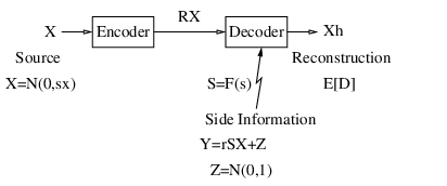
Suppose the side-information channel has $M$ discrete fading states. Let the probability distribution of $S$ be given as follows:

where the $s_{i}$’s are enumerated in ascending order $0\leq s_{1}<s_{2}<\dotsb<s_{M}$. Let $Y^{\prime}_{i}$ denote the side information under fading state $s_{i}$

Note that the set of side information random variables are stochastically degraded. Let $\hat{X}_{i}$ be the reconstruction when side information $Y^{\prime}_{i}$ is available at the decoder, and $D_{i}$ be the corresponding squared error distortion. The minimum expected distortion under rate constraint $R_{X}$ is then given by

where $\mathbf{p}\triangleq[p_{1}\dots p_{M}]^{T}$, $\mathbf{D}\triangleq[D_{1}\dots D_{M}]^{T}$, and $R(\mathbf{D})$ is the rate–distortion function that simultaneously satisfies the distortion set $\mathbf{D}$.

The rate–distortion function that dictates the rate required to simultaneously satisfy a set of distortion constraints associated with a set of degraded side-information random variables is given by Heegard and Berger in [3] (an alternate form for $M=2$ is described in [22]). When the side information random variables satisfy the degradedness condition $X\leftrightarrow Y_{M}\leftrightarrow Y_{M-1}\leftrightarrow\dotsb\leftrightarrow Y_{1}$, the rate–distortion function is

where $W_{1}^{i}$ denotes the vector $W_{1},\dotsc,W_{i}$. The minimization takes place over $P(\mathbf{D})$, the set of all $W_{1}^{M}$ jointly distributed with $X,Y_{1}^{M}$ such that:

and there exists decoding functions $\hat{X}_{i}(Y_{i},W_{1}^{i})$’s under given distortion measures $d_{i}$’s that satisfy

As noted in [3], since $R_{\HB}(\mathbf{D})$ depends on $X,Y_{1}^{M}$ only through the marginal distribution $p(x,y_{i})$, $i=1,\dotsc,M$, the degradedness of the side information need not be physical. We construct $Y_{1}^{M}$ to have the same marginals as ${Y^{\prime}}_{1}^{M}$ by setting $p(y_{i}|x)=p(y^{\prime}_{i}|x)$, $i=1,\dotsc,M$. The rate–distortion function $R(\mathbf{D})$ in (3) is then given by the Heegard–Berger rate–distortion function (4) with squared error distortion measures $d_{i}(X,\hat{X}_{i})=(X-\hat{X}_{i})^{2}$.

The Heegard–Berger rate–distortion function $R_{\HB}(D_{1},\dotsc,D_{M})$ for a Gaussian source under squared error distortion is given in [3, 9, 10]. For $M=2$, [3] describes the Gaussian rate–distortion function where the worst fading state corresponds to no side information, and [9] considers side information with different quality levels. The Gaussian Heegard–Berger rate–distortion function is considered in [10] for $M>2$. However, the representations of $R_{\HB}(D_{1},\dotsc,D_{M})$ described in [3, 9] are characterized by exponentially-many distinct regions, and [10] involves optimal Gaussian random variables whose variances are determined by an algorithmic procedure. These characterizations, though complete, are not amenable to efficient minimization of the expected distortion. In this section, we derive a representation for $R_{\HB}(D_{1},\dotsc,D_{M})$ that can be incorporated in an optimization framework. In particular, instead of describing the achievable distortion set by its exponentially-many segments of boundaries, we construct a characterization that comprises a sequence of convex inequalities, each relating the achievable distortion between two adjacent fading states. Consequently, we formulate the distortion minimization as a convex optimization problem where the number of variables and constraints are linear in $M$. First we consider the case when the side-information channel has only two discrete fading states ($M=2$); in Section III-C we extend the analysis to multiple fading states where $M>2$.

When the side-information channel has two fading states, the encoder constructs a source-coding scheme that consists of two layers of codewords. The base layer is designed to be decodable under either channel condition, while the top layer is only decodable under the more favorable channel realization. We derive the rate requirements of the two codeword layers, and optimally allocate the encoding rate $R_{X}$ between them to minimize the expected distortion. For $M=2$, the Heegard–Berger rate–distortion function is given by

For a Gaussian source under a squared error distortion measure, a jointly Gaussian codebook is optimal [3, 9, 10]. When $W_{1}^{M},X$ are jointly Gaussian, the mutual information expressions in (7) evaluate to

where $\log$ is the natural logarithm, and (9) follows from expanding the conditional variance expressions by applying Lemma 1 and Corollary 1. The proof of Lemma 1 is given in Appendix A.

To characterize the Heegard–Berger rate–distortion function $R_{\HB}(D_{1},D_{2})$, we substitute (9) in (7), and minimize over $W_{1},W_{2}$

Note that $s_{2}>s_{1}\geq 0$ by assumption. Accordingly, in the inner minimization in (12), $R_{\HB}(D_{1},D_{2})$ is decreasing in $\mathrm{VAR}[X|Y_{2},W_{1},W_{2}]$. Hence the choice of $W_{2}$ is optimal when $\mathrm{VAR}[X|Y_{2},W_{1},W_{2}]$ is increased until one of its upper bound constraints is tight

The optimal $W_{2}^{*}$ that achieves (13) is presented subsequently. The first term in the $\min(\cdot)$ expression in (13) follows from the non-negativity of the mutual information $I(X;W_{2}|Y_{2},W_{1})$, and the second one follows from the distortion constraint on $\hat{X}_{2}$ as given in (6)

Applying Corollary 1, the first term in (13) evaluates to

Under optimal $W_{2}$, therefore, the Heegard–Berger rate–distortion function in (12) reduces to

The maximization over $W_{1}$ in (16) has a similar structure as the one previously considered in (13). Specifically, $R_{\HB}(D_{1},D_{2})$ in (16) is decreasing in $\mathrm{VAR}[X|Y_{1},W_{1}]$. Hence $W_{1}$ is optimal when $\mathrm{VAR}[X|Y_{1},W_{1}]$ is increased until it meets one of its upper bound constraints

where the first term in (17) follows from the non-negativity of $I(X;W_{1}|Y_{1})$, and the second one from the distortion constraint on $\hat{X}_{1}$

Next, we consider the construction of $W_{1},W_{2}$ that achieves the rate–distortion function, namely, jointly Gaussian random variables with conditional variances that satisfy (13), (17). We construct the optimal distribution $W_{1}^{*},W_{2}^{*}$ as follows:

where $N_{i}\sim\mbox{ i.i.d. }\mathcal{N}(0,1)$, $i=1,2$, is independent from $X,Y_{1},Y_{2}$, and $a_{1},a_{2}$ are nonnegative scalars whose values are to be specified. For notational convenience, we define

where (22) follows from (17). Substitute (19) in (21), and $a_{1}$ evaluates to

Similarly, to identify the optimal $W_{2}^{*}$, we define

which follows from (13), (15). Substitute (20) in (24), and $a_{2}$ evaluates to

To provide an interpretation regarding the source encoding rates under different fading states of the side-information channel, we introduce the notations

where (28), (30) follow from expanding the mutual information expressions applying (23), (26). We interpret $R_{1}$ as the rate of a source coding base layer that describes $X$ when the side-information quality is that of $Y_{1}$ or better. On the other hand, $R_{2}$ is the rate of a top layer that describes $X$ only when the decoder has the better side information $Y_{2}$. Finally, we substitute (28), (30) in (7) to obtain the two-layer Heegard–Berger rate–distortion function

where $V_{1},V_{2}$ are as defined in (21), (24) above. The derivation of (32) depends on the side information only through the marginals $p(y_{i}|x)$’s; therefore, the rate–distortion function applies as well to the stochastically degraded side information $Y^{\prime}_{M},\dotsc,Y^{\prime}_{1}$.

Under a source-coding rate constraint of $R_{X}$, the Heegard–Berger feasible distortion region is described by

The distortion regions under different values of $R_{X}$ are illustrated in Fig. 2. Setting $R_{\HB}(D_{1},D_{2})$ $=$ $R_{X}$, the dominant boundary of $\{(D_{1},D_{2})\}$ defines the Pareto optimal trade-off curve (shown in bold in Fig. 2) between the two distortion constraints on $\hat{X}_{1}$ and $\hat{X}_{2}$, which is given by

over the interval

We find the optimal operating point on the Pareto curve to minimize the expected distortion

In Section III-C, it is shown that the above minimization is a convex optimization problem. Hence the Karush–Kuhn–Tucker (KKT) conditions are necessary and sufficient for optimality. Moreover, $\mathcal{D}(R_{X})$, being the sublevel set of a convex function, is a convex set. After substituting (34) in (36), from the KKT optimality conditions, we obtain the optimal base layer distortion

where $(x)_{[a,\,b]}$ denotes the projection

and the distortion and its boundaries are given by

The optimal top layer distortion $D_{2}^{*}$ is given by

where

The corresponding optimal rate allocation $R_{1}^{*},R_{2}^{*}$ can be found as given in (28), (30).

The optimal rate allocation and the corresponding minimum expected distortion are plotted in Fig. 3 and Fig. 4, respectively, for $R_{X}=1$, $\sigma_{X}^{2}=1$, and $s_{1}=0\,\dB$. Note that $R_{2}^{*}$, the rate allocated to the top layer, is not monotonic with the side-information channel condition. As fading state $s_{2}$ improves, $R_{2}^{*}$ increases to take advantage of the better side-information quality. However, when $s_{2}$ is large, $R_{2}^{*}$ begins to decline as the expected distortion is dominated by the worst fading state. In addition, the optimal rate allocation is heavily skewed towards the lower layer: $R_{2}^{*}>0$ only when $p_{2}$ is large.

The rate–distortion function (32) extends directly to the case when the side-information channel has multiple discrete fading states: $S=s_{i}$ with probability $p_{i}$, where $i=1,\dotsc,M$, with $0\leq s_{1}<\dotsb<s_{M}$, and $M>2$. The Heegard–Berger rate–distortion function for $M>2$ can be characterized by a similar representation as that given in (32) for $M=2$. Specifically, we construct the optimal distribution for the auxiliary random variable $W_{i}^{*}$’s to be given by

where $N_{i}\sim\mbox{ i.i.d. }\mathcal{N}(0,1)$, and $a_{i}$’s are nonnegative scalars whose values are to be specified. The rate of the $i\,$th layer is

where

and $s_{0}\triangleq 0$, $V_{0}\triangleq\sigma_{X}^{2}$ for convenience in notations. In the above, (50) follows from the non-negativity of $I(X;W_{i}|Y_{i},W_{1},\dotsc,W_{i-1})$ and the distortion constraint (6). The $a_{i}$ that achieves (49) is determined from (50), which evaluates to

As $R_{\HB}(\mathbf{D})=\sum_{i=1}^{M}R_{i}$, we substitute (48) in (4) to obtain the rate–distortion function

where the $V_{i}$’s are as given in (50).

Under multiple fading states, however, a closed-form expression for the minimum expected distortion $\mathrm{E}[D]^{*}$ does not appear analytically tractable. Nevertheless, the expected distortion minimization in (3) can be formulated as the following convex optimization problem:

where $\mathds{R}_{++}$ denotes the set of positive real numbers. In (53) above, the cost function $J(\cdot)$ may be any arbitrary function that is convex in $D_{1},\dotsc,D_{M}$. The constraint (55) prescribes the feasible Heegard–Berger distortion region under the source-coding rate constraint $R_{X}$. The constraints (56) and (57) derive from writing out the two upper bounds for each $V_{i}$, as described in (50), as two separate inequality constraints. The equality in (50) may be written as inequality constraints since there is an optimal solution where for each $i$ at least one of (56) or (57) is tight. Specifically, the left-hand side of the Heegard–Berger constraint in (55) is monotonically decreasing in $V_{i}$’s. Hence for a given optimal $\{V_{i}^{*},D_{i}^{*}\}$, if neither (56) nor (57) is tight, $V_{i}^{*}$ may be increased to strictly enlarge the feasible set of $\{D_{1},\dotsc,D_{M},\,V_{1},\dotsc,V_{M}\}\backslash\{D_{i},V_{i}\}$.

See Appendix B for the proof of Proposition 1. Convexity implies that a local optimum is globally optimal, and its solution can be efficiently computed by standard convex optimization numerical techniques, for instance, by the interior-point method [23, 24]. Moreover, the optimization problem (53)–(57) has $2M$ variables and $2M+1$ inequality constraints, which are linear in the number of side-information channel fading states $M$.

In the case where the cost function $J(D_{1},\dotsc,D_{M})$ is non-decreasing in each component $D_{i}$, the constraints (57) may be taken as tight: if at their optimal values $V_{i}^{*}<D_{i}^{*}$, then $D_{i}^{*}$ may be decreased without violating feasibility nor increasing the cost function. In particular, in the remainder of the paper, we consider minimizing the expected distortion:

In this case, the optimization problem can be specified more compactly as

where in (62) similarly $D_{0}\triangleq\sigma_{X}^{2}$. For convenience in stating the optimization problem, in (61), and in the remainder of the paper, $\log$ refers to the extended-value logarithmic function, where it takes on the value $-\infty$ for non-positive arguments. Then the feasibility constraints (61), (62) imply $D_{i}>0$, $i=1,\dotsc,M$, and the domain qualification $\{D_{i}\in\mathds{R_{++}}\}$ is thus omitted from (60). The positivity of $D_{i}$ can be shown as follows. Note that (61) implies

Consider $i=M-1$. Suppose $D_{M-1}<0$, then (64) rearranges to $(D_{M-1}^{-1}+s_{M}-s_{M-1})^{-1}<0$, which contradicts (62), (63): $(D_{M-1}^{-1}+s_{M}-s_{M-1})^{-1}\geq D_{M}>0$. Next, suppose $D_{M-1}=0$. Applying $\lim_{D_{M-1}\rightarrow 0^{+}}$ on (62), the inequality becomes: $D_{M}\leq 0$, which contradicts (63). Therefore, $D_{M-1}>0$, and similar arguments apply for $D_{M-2},\dotsc,D_{1}$.

Suppose the side-information channel has infinitely many discrete fading states $\{s_{1},s_{2},\dotsc\}$ with $0\leq s_{1}<s_{2}<\cdots$. Let $p_{i}$ denote the probability the side-information channel takes on state $s_{i}$, with $\sum_{i=1}^{\infty}p_{i}=1$. Let $\mathbf{D}\triangleq[D_{1}\;D_{2}\;\dots]^{T}$ denote the set of distortion variables induced by the rate allocation scheme. Note that the Heegard–Berger rate–distortion function extends to the set of infinitely many degraded fading states. We assume the total encoding rate $R_{X}$ is finite, and hence so is the rate $R_{i}$ for each fading state. For admissibility, the random coding argument in [3, Section III] applies for each of the fading states, and the converse in [3, Section VII] depends only on the total encoding rate but not the number of fading states. Furthermore, it can be shown using the same approach in [10] that the optimality of Gaussian solution for the Gaussian side information Heegard-Berger problem still holds for this scenario. The expected distortion minimization problem is given by

The rate constraint (77) follows from (48). Recall that the extended-value logarithm takes on $-\infty$ for non-positive arguments. The constraint (77) then implies $D_{i}>0$; hence the domain $D_{i}>0$ is not explicitly stated in the optimization problem. In Appendix C, it is shown that (75)–(78) is a convex problem, and its KKT optimality conditions and dual function are given in Appendix D. Next, we show that the single-layer rate allocation (74) is expected-distortion–minimizing in (75)–(78) under some conditions.

Consider the single-layer rate allocation (74) with $\bar{s}=s_{i}$ for some $i$. Relating $\mathcal{R}_{\bar{s}}$ to the induced distortion set (48), we have

with the single-layer expected distortion given by

In the notation, the overbar accent is used to represent single-layer rate allocation. To determine optimality, we apply the KKT complementary slackness condition (110) on (79) above, and it stipulates that

Next, we apply the KKT gradient conditions (109) on (79), (81), and the dual variables $\bar{\lambda}_{i}$ are given as follows:

References

- [1] A. D. Wyner and J. Ziv, “The rate-distortion function for source coding with side information at the decoder,” IEEE Trans. Inf. Theory, vol. 22, no. 1, pp. 1–10, Jan. 1976.
- [2] S. Shamai (Shitz) and A. Steiner, “A broadcast approach for a single-user slowly fading MIMO channel,” IEEE Trans. Inf. Theory, vol. 49, no. 10, pp. 2617–2635, Oct. 2003.
- [3] C. Heegard and T. Berger, “Rate distortion when side information may be absent,” IEEE Trans. Inf. Theory, vol. 31, no. 6, pp. 727–734, Nov. 1985.
- [4] A. D. Wyner, “The rate-distortion function for source coding with side information at the decoder—II: General sources,” Inform. Contr., vol. 38, pp. 60–80, Jul. 1978.
- [5] R. M. Gray, “A new class of lower bounds to information rates of stationary sources via conditional rate-distortion functions,” IEEE Trans. Inf. Theory, vol. 19, no. 4, pp. 480–489, Jul. 1973.
- [6] R. Zamir, “The rate loss in the Wyner–Ziv problem,” IEEE Trans. Inf. Theory, vol. 42, no. 6, pp. 2073–2084, Nov. 1996.
- [7] M. Fleming and M. Effros, “On rate-distortion with mixed types of side information,” IEEE Trans. Inf. Theory, vol. 52, no. 4, pp. 1698–1705, Apr. 2006.
- [8] Y. Steinberg and N. Merhav, “On successive refinement for the Wyner-Ziv problem,” IEEE Trans. Inf. Theory, vol. 50, no. 8, pp. 1636–1654, Aug. 2004.
- [9] C. Tian and S. N. Diggavi, “On multistage successive refinement for Wyner–Ziv source coding with degraded side informations,” IEEE Trans. Inf. Theory, vol. 53, no. 8, pp. 2946–2960, Aug. 2007.
- [10] ——, “Side-information scalable source coding,” IEEE Trans. Inf. Theory, vol. 54, no. 12, pp. 5591–5608, Dec. 2008.
- [11] M. Feder and N. Shulman, “Source broadcasting with unknown amount of receiver side information,” in Proc. IEEE Inform. Theory Workshop, Bangalore, India, Oct. 2002, pp. 127–130.
- [12] N. Shulman and M. Feder, “Static broadcasting,” in Proc. IEEE Int. Symp. on Inform. Theory, Sorrento, Italy, Jun. 2000, p. 23.
- [13] C. Tian, A. Steiner, S. Shamai (Shitz), and S. N. Diggavi, “Successive refinement via broadcast: Optimizing expected distortion of a Gaussian source over a Gaussian fading channel,” IEEE Trans. Inf. Theory, vol. 54, no. 7, pp. 2903–2918, Jul. 2008.
- [14] C. T. K. Ng, D. Gündüz, A. J. Goldsmith, and E. Erkip, “Distortion minimization in gaussian layered broadcast coding with successive refinement,” IEEE Trans. Inf. Theory, vol. 55, no. 11, pp. 5074–5086, Nov. 2009.
- [15] A. Steiner and S. Shamai (Shitz), “Achievable rates with imperfect transmitter side information using a broadcast transmission strategy,” IEEE Trans. Wireless Commun., vol. 7, no. 3, pp. 1043–1051, Mar. 2008.
- [16] S. Shamai (Shitz), S. Verdú, and R. Zamir, “Systematic lossy source/channel coding,” IEEE Trans. Inf. Theory, vol. 44, no. 2, pp. 564–579, Mar. 1998.
- [17] D. Gunduz, J. Nayak, and E. Tuncel, “Wyner–Ziv coding over broadcast channels using hybrid digital/analog transmission,” in Proc. IEEE Int. Symp. on Inform. Theory, Toronto, Canada, Jul. 2008, pp. 1543–1547.
- [18] J. Nayak, E. Tuncel, and D. Gündüz, “Wyner–Ziv coding over broadcast channels: Digital schemes,” IEEE Trans. Inf. Theory, vol. 56, no. 4, pp. 1782–1799, Apr. 2010.
- [19] P. Ishwar, R. Puri, K. Ramchandran, and S. S. Pradhan, “On rate-constrained distributed estimation in unreliable sensor networks,” IEEE J. Sel. Areas Commun., vol. 23, no. 4, pp. 765–775, Apr. 2005.
- [20] J. Chen and T. Berger, “Robust distributed source coding,” IEEE Trans. Inf. Theory, vol. 54, no. 8, pp. 3385–3398, Aug. 2008.
- [21] O. Simeone, O. Somekh, E. Erkip, H. V. Poor, and S. Shamai (Shitz), “Robust communication via decentralized processing with unreliable backhaul links,” IEEE Trans. Inf. Theory, vol. 57, no. 7, pp. 4187–4201, Jul. 2011.
- [22] A. H. Kaspi, “Rate-distortion function when side-information may be present at the decoder,” IEEE Trans. Inf. Theory, vol. 40, no. 6, pp. 2031–2034, Nov. 1994.
- [23] J. Renegar, A Mathematical View of Interior-Point Methods in Convex Optimization. Philadelphia, PA: MPS-SIAM, 2001.
- [24] S. Boyd and L. Vandenberghe, Convex Optimization. Cambridge, UK: Cambridge University Press, 2004.
- [25] G. L. Stüber, Principles of Mobile Communication. Norwell, MA: Kluwer Academic Publishers, 2000.
- [26] T. M. Cover and J. A. Thomas, Elements of Information Theory. New York, NY: Wiley-Interscience, 1991.
- [27] J. N. Laneman, E. Martinian, G. W. Wornell, and J. G. Apostolopoulos, “Source-channel diversity for parallel channels,” IEEE Trans. Inf. Theory, vol. 51, no. 10, pp. 3518–3539, Oct. 2005.
- [28] M. Katz and S. Shamai (Shitz), “Cooperative schemes for a source and an occasional nearby relay in wireless networks,” IEEE Trans. Inf. Theory, vol. 55, no. 11, pp. 5138–5160, Nov. 2009.
- [29] D. G. Luenberger, Optimization by Vector Space Methods. New York, NY: Wiley-Interscience, 1969.