Cavity-induced giant Kerr nonlinearities in a driven -type atom
Abstract
We discuss a simple and experimentally realizable model for creation of enhanced Kerr nonlinearities accompanied by vanishing absorption. The model involves a -type atom subjected to a strong drive laser, a weak probe laser and coupled to a single-mode cavity field. Working in the bad-cavity limit, we find that the simultaneous coupling of the cavity field to both atomic transitions creates a coherence between the transitions and thus can lead to quantum interference effects. We investigate the influences of the cavity field frequency, the cavity field-atom coupling constants and the atomic decay constants on the linear and the third-order (Kerr) nonlinear susceptibilities. We predict giant Kerr nonlinearities with vanishing absorption and attribute this effect to the combination of the Purcell effect and the cavity-induced quantum interference.
pacs
42.50.Gy, 42.65.-k1 Introduction
A great deal of attention has been focused recently on the creation of strong nonlinear effects in single coherently prepared multi-level atoms [1, 2]. The motivation for this interest is to fabricate an atomic medium with giant nonlinear properties produced with relatively low light powers. A particular attention has been paid to the third-order Kerr-type nonlinearities which play an important role in nonlinear optics and have many fascinating applications in different areas of physics ranging from phase modulation [3], generation of optical solitons [4], optical switching [5] to optical communication and computing [6]. Important for practical applications is to achieve enhanced or giant Kerr nonlinearities in an atomic medium with significantly reduced or even completely cancelled absorption rate for the propagating light beam. Imamoǧlu et al. [7] have proposed a scheme to produce giant Kerr nonlinearities together with reduced absorption, by using quantum interference effects related to electromagnetically induced transparency. In a four-level double-dark resonance system, Kerr nonlinearity can be enhanced several orders of magnitude accompanied by vanishing linear absorption under the condition of the effective interaction of double dark resonances [8]. A number of different atomic schemes have been suggested to achieve a large nonlinearity with vanishing absorption [9, 10]. More recently, Niu and Gong [11] and Yan et al. [12] have shown that the Kerr nonlinearity can be enhanced with vanishing linear and nonlinear absorptions due to the spontaneously generated coherence [13].
The major obstacle in experimental investigations of the nonlinear properties of multi-level atoms is the difficulty to find suitable systems to create quantum interference effects between atomic transitions responsible for the cancelation of the absorption of a propagating field. Most of the schemes proposed have assumed that the quantum interference occurs between two transitions with parallel or anti-parallel dipole moments. In atoms with quantum states close in energy the dipole moments are usually perpendicular. Therefore, several schemes have been suggested to engineer quantum interference effects in atoms with perpendicular dipole moments. Most of the schemes suggests to use single-mode optical cavities with preselected polarization in bad cavity limit [14, 15, 16]. Bermel et al. [17] have found that the Purcell effect [18] can substantially influence the Kerr nonlinearity. Brandão et al. [19] proposed a method to produce self- and cross-Kerr photonic nonlinearities using light induced Stark shifts arising from the interaction of a cavity mode with atoms. In addition to the Purcell effect which is substantial in optical cavities, where spontaneous transitions occur only at selected frequencies, a cavity-induced quantum interference is expected to arise which is analog of the spontaneously generated interference [20]. Thus, a question arises, to what extent a combination of the Purcell effect and the cavity-induced interference effects will affect the susceptibility of driven -type three-level atom. The purpose of this paper is to address this question and discuss in detail the possibility of obtaining giant Kerr nonlinearities.
We consider a three-level atom in the configuration in which one of the two dipole allowed transitions is driven by a strong laser field while the other is probed by a weak beam. The atomic transitions are simultaneously coupled to a tunable single-mode cavity. Our interest will be centered principally on the effect of the cavity on the third-order susceptibility and determine if the driven system possesses enhanced or giant nonlinearities accompanied by vanishing absorption. The paper is organized as follows. In Section 2, we introduce our model and outline the major steps in the derivation of the equations of motion for the density matrix elements. The iterative analytical solution for the coherences determining the susceptibility is presented in Section 3. The results are presented graphically and discussed in Section 4. We show the influences of the cavity field frequency, the cavity field-atom coupling constants and the atomic decay constants on the real and imaginary parts of the linear and nonlinear susceptibilities. We summarize our results in Section 5.
2 Theoretical Model
We consider a -type three-level atom composed of two excited states and coupled to a common ground state by transition dipole moments and , respectively. The atom is located inside a single-mode cavity field of frequency and polarization , as shown in Fig. 1.

The polarization is chosen such that the cavity field is simultaneously coupled to both atomic transitions with the coupling strengths and , respectively. The atomic transition is driven by a strong laser field of frequency , whereas the transition is probed by a weak tunable laser beam of frequency . The cavity mode is damped at the rate , whereas the atomic transitions are damped by spontaneous emission to the modes other than the cavity mode at the rates and , respectively. In a frame rotating at the frequency , the master equation of the density operator of the overall system (the atom and the cavity field) is of the form
| (1) |
where
| (2) | |||||
is the unperturbed Hamiltonian of the coherently driven and weakly probed atom,
| (3) |
is the Hamiltonian of the cavity field,
| (4) |
is the interaction Hamiltonian of the cavity field with the atomic transitions, and
| (5) |
are dissipative terms describing the damping of the atomic transitions by spontaneous emission and of the field by cavity decay.
Here, and are the annihilation and creation operators for the cavity field, are the atomic operators, is the frequency difference between the atomic transitions, , and are the detunings of the atomic frequency , the probe beam frequency and the cavity frequency from the driving laser frequency . The parameters, and are the (real) Rabi frequencies of the driving laser field of amplitude and of the probe beam of amplitude .
In writing the master equation (1), we have assumed that the atomic dipole moments are not orthogonal to each other, which results in the cross damping terms between the atomic transitions. These terms lead to quantum interference between the two transitions and are determined by the so-called cross damping parameter , where is the angle between and . When the dipole moments are parallel ( =0), the cross damping parameter is maximal with , whilst when the dipole moments are perpendicular [20]. Quantum interference has been studied intensively over years and has revealed new phenomena of both conceptual and practical importance. It has been shown that interference between atomic transitions induced by external fields or by spontaneously created atomic coherence can lead to novel phenomena such as electromagnetically induced transparency, lasing without inversion, enhanced index of refraction and also nonlinear processes such as enhanced the Kerr nonlinearities. However, most of the predicted quantum interference effects have so far eluded observation, as it is very unlikely to find isolated atoms with two non-orthogonal dipole moments and states close in energy. Therefore, we propose an alternative scheme where one can engineer coherence between atomic transitions with perpendicular dipole moments by coupling the transitions to a single-mode cavity field. As we shall see, crucial for the creation of the coherence is to couple the cavity mode simultaneously to both of the atomic transitions. In practice, it can be easily achieved by setting a cavity-field polarization making, for example, an angle with the direction of the atomic dipole moment and that simultaneously forms the angle with the dipole moment .
The master equation (1) we have started with is written in the basis of the atomic states. Since the atomic transition is driven by a strong laser field, it prompts us to introduce dressed states which provide a good approach for studying the problem. The dressed states are eigenstates of the Hamiltonian and are defined by the eigenvalue equation
| (6) |
whose the eigenvalues and corresponding eigenstates, in the limit of a weak probe beam , are
| (7) |
where
| (8) |
and is the detuned Rabi frequency of the driving field.
We now introduce the interaction between the dressed atom and the cavity field and work in the bad cavity limit [15, 21, 22], in which the cavity decay dominates over the coupling strengths and the atomic decay rates and , i.e.
| (9) |
Such a feature implies that the cavity mode response to the standard vacuum reservoir is much faster than that produced by its interaction with the atom. In other words, the cavity field forms a finite bandwidth (Markovian) vacuum reservoir.
Working in the bad cavity limit, we can adiabatically eliminate the cavity variables. This yields a master equation where the damping terms have a structure dependent on the difference between the cavity field and the dressed-atom transition frequencies. Details of the adiabatic approximation have been presented in ref. [15]. Here, we will apply such approach to study the linear and nonlinear responses of the system to a weak probe field.
From the cavity-modified master equation, the equation of motion for the atomic density matrix elements, written in the dressed state basis, are of the form
| (10) | |||||
| (11) | |||||
| (12) | |||||
| (13) | |||||
| (14) |
where
| (15) |
are the quantum interference terms,
| (16) |
are the cavity modified damping rates between the dressed states,
| (17) |
are the cavity modified damping rates of the coherence, with
| (18) |
and
| (19) |
are the dressed atom coherence in a rotating frame oscillating with frequency . Equations (10)14) are valid for any value of the cavity detuning , and the upper levels splitting comparable to half of the Rabi frequency, i.e. for . Physically, the approximation of corresponds to the case when the probe level is degenerate or nearly degenerate with respect to the dressed state . In this case, the resultant degeneracy gives rise to maximal quantum interference effects. Moreover, under this approximation, and .
The parameters appearing in the equations of motion have simple physical interpretations. The parameters are quantum interference terms. They contain contributions of both, spontaneously generated and cavity effects, which clearly illustrate an analogy between the cavity engineered and the spontaneously induced coherence [13, 15, 20]. Thus, the cavity with large decay rate strongly enhances quantum interference effects.
The parameters represent the transition rates between the dressed states of the system and are the damping rates of the coherence. Note that the parameters are dependent on the Rabi frequency of the driving field and are resonant when the cavity frequency is tuned to . It means that spontaneous emission and quantum interference dominate at five frequencies. The sensitivity of the coefficients on is known in the literature as the Purcell effect. Thus, in the system considered here, both the Purcell and the cavity-induced quantum interference effects play an important role in the dynamics and properties of the system.
One can notice from (10)(14) that the coefficients in the differential equations are dependent on time. In fact, there is no reference frame in which the coefficients would be time independent. It is clear that the time dependence of the coefficients is brought here by the interference terms. As the result of the time dependence, special mathematical techniques must be employed to solve the set of the equations of motion. In the next section, we will solve the set of equations for the steady state density matrix elements using the Floquet technique.
3 Linear and nonlinear (Kerr) susceptibilities
Our purpose of this paper is to demonstrate that the combined effect of the Purcell and the cavity-induced quantum interference phenomena can create giant linear and nonlinear susceptibilities in the three-level system. Note that the cavity-induced quantum interference effects are more flexible to the parameters than those induced by the spontaneously generated coherence. The latter depend solely on the angle between the dipole moments of the two atomic transitions. The former depend on the Rabi frequency of the driving field, damping rates of the atomic transitions, and the detunings of the fields from their resonances. This makes the cavity system more practical for creation of quantum interference effects than that induced by spontaneously created coherence.
It is well known that the response of the atomic medium to the probe field is governed by its polarization , which can be expressed in terms of the complex susceptibility or related to the elements of the density matrix of the system as
| (20) |
where is the number density of the atoms, and is the atomic coherence on the probed transition. The task then is to determine the atomic coherence , or equivalently and , which could be found by solving the set of equations (10)(14). In the stationary limit , we may set all of the derivatives to zero and obtain a set of algebraic equations for the density matrix elements. However, the set of equations retains the time dependence through the factors . Therefore, to solve the system of equations (10)(14), we employ the Floquet method by expressing the density matrix elements as Fourier series in terms of amplitudes that oscillate at the probe detuning and its harmonics. As we are interested in the response of the system to a weak probe field, we also make an expansion of the density matrix elements in terms of the powers of the probe field. These two decompositions combined together are given by the relation [23]
| (21) |
where the expansion in the powers of is given in terms of a dimensionless parameter that can take on values ranging continuously from zero (no perturbation) to one (the full perturbation).
Since the atomic coherence on the probe transition oscillates as , the stationary properties of the first and third-order susceptibilities are determined by the harmonics and , respectively. Therefore according to Eq. (10) the susceptibilities and can be expressed in terms of the first and third order coherence of the probe transition as
| (22) | |||||
| (23) |
The linear and nonlinear susceptibilities can be conveniently expressed in the form
| (24) |
where we have introduced the normalized real and imaginary parts of that determine the index of refraction and the absorption coefficient, respectively. Evidently, the normalized parts of are independent of the probe field strength . This allows the susceptibilities to be arbitrary large since the only approximation made here is an assumption of weak probe beam strengths. Note that implies lossless propagation of the probe field, implies linear refraction of the probe beam, and implies nonlinear intensity dependent (Kerr) refraction.
Upon substitution of (21) into (10)(14) and after comparing terms of the same powers in , we obtain an infinite set of equations for the Fourier harmonics with time independent coefficients. Despite of the complexity, the system of the coupled equations is easily solved for the steady state by an iteration in terms of the powers of the probe field amplitude. The analytical iterative solution for the order harmonics of the coherence appearing in (22) and (23) are of the form
| (25) | |||||
| (26) | |||||
where the analytical solutions for the auxiliary harmonics are quite lengthy and are listed in the Appendix. It follows from the explicit solutions (25) and (26) that the magnitudes of the harmonics are proportional to , which ensures that their magnitudes are small even if the normalized susceptibilities and are large, since the probe beam strength is considered here to be weak, . This justifies the power expansion (21).
4 Discussion of the results
We now proceed to perform detailed analysis of the the linear and nonlinear susceptibilities by graphically displaying the real and imaginary parts of and for a wide range of the important parameters. We are particularly interested in the possibility of creation of giant Kerr nonlinearities accompanied by zero linear and nonlinear absorptions. In what follows, we assume for simplicity that the driving laser field is on resonance with the atomic transition , i.e., .
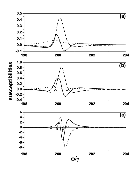
In Fig. 2, we illustrate the variation of the real and imaginary parts of and the imaginary part of with the probe field detuning from resonance with the transition . We choose the Rabi frequency of the driving field such that . In this particular case, the dressed state and the probe state are degenerated in the energies, which is the maximal quantum interference configuration. All of the parameters are measured in units of the damping rate through out these figures. Part (a) of the figure shows the susceptibilities for . This corresponds to the cavity field tuned to the central component of the dressed transitions. We see that the susceptibilities exhibit resonance structures in the vicinity of the frequency . As we have already mentioned, at this frequency the quantum interference is maximal. The nonlinear (Kerr) susceptibility is enhanced, but at the same time the linear and nonlinear absorptions are large. Even at the frequency where the nonlinear absorption, Im, vanishes, the linear absorption Im is large with the magnitude comparable to the magnitude of the Kerr nonlinearity. This is not desirable for a practical application since the probe beam could be completely absorbed over a short distant of propagation inside the atomic medium. Therefore, we now proceed to check if one could achieve a large Kerr nonlinearity accompanied by vanishing linear and nonlinear absorption by varying parameters of the system. A close inspection of the analytical expressions (25) and (26) shows that the absorption rate of the probe beam depends on the difference between the populations of the lower and upper levels of the probe transition which, on the other hand, depends on the detuning . Thus, we expect that the transparency of the propagation of the probe beam could be improved by applying the Purcell effect, i.e. by varying the detuning to match the cavity frequency with the frequency of one of the Rabi sidebands of the driven transition.
Parts (b) and (c) of the figure show how the susceptibilities are modified when the cavity detuning is varied. There a few significant changes observed in the behavior of the susceptibility. Firstly, the Kerr nonlinearity becomes enhanced by few orders in magnitude when the detuning approaches the value , corresponding to the tuning of the cavity field to the Rabi sideband of the driven transition. Secondly, the Kerr nonlinearity varies rapidly with the probe frequency. However, the most important change in the behavior of the susceptibility is that at the frequency, indicated by a dot D, where the Kerr nonlinearity is maximal, the nonlinear absorption vanishes completely and the linear absorption is negligibly small. In other words, the system is transparent for the probe beam at the frequency where the Kerr nonlinearity is maximal. We may conclude that by tuning the cavity field to one of the Rabi sidebands, one can achieve a giant Kerr nonlinearity accompanied by vanishing absorption.

We have seen that a combination of the maximal quantum interference and the Purcell effect is crucial for creation of a giant Kerr nonlinearity accompanied by vanishing absorption. To illustrate the importance of maintaining the maximal quantum interference, we now slightly detune the dressed state from the probed atomic state , so that the states become non-degenerate. It is well known, that quantum interference effects degrade when interfering energy states are non-degenerate. Let us see how this can affect the Kerr nonlinearity and the transparency of the atomic medium. In Fig. 3, we plot the imaginary parts of and and the real part of for the same parameters as in Fig. 2(c), but with . In this case, the state is detuned from the state by , that is the cavity field is detuned from the dressed atom frequencies. It is easy to see from (18) that the effect of detuning the cavity field from the dressed atom frequencies is to reduce the magnitude of quantum interference terms. Part (a) of the figure shows that the linear absorption is small at all frequencies, but within the region when the Kerr nonlinearity is enhanced, the nonlinear absorption is very large. Thus, the atomic medium becomes highly absorbing for the probe beam when the quantum interference effects are reduced.
To illustrate further the effectiveness of the enhancement of the Kerr nonlinearity by quantum interference, we plot in part (b) of the figure the ratios and for the presence and the absence of quantum interference. We see that at the frequency the ratios are maximal in the presence of quantum interference and vanish completely in the absence of quantum interference. Note that the maxima of the ratios occur at frequencies slightly shifted from the resonance . This is because after adiabatically eliminating the cavity field operators in the bad cavity limit, the remaining cavity effects are not only to affect the atomic damping rates but also to induce a small energy shifts for the levels and . We may conclude that the enhanced Kerr nonlinearity with relatively vanishing linear and nonlinear absorptions is a signature of the cavity-induced quantum interference effects.

We now proceed to check the importance of other parameters of the system such as the atomic decay rate and the cavity field-atom coupling constant . Figure 4(a) illustrates the susceptibility for the same parameters as in Fig. 2(c), but . It is evident that at this small damping rate, the linear absorption is zero at all frequencies, while the nonlinear absorption vanishes at two frequencies, indicated by dots E and F. At these frequencies the Kerr nonlinearity is large. In particular, at the point F, the Kerr nonlinearity is about one order higher in magnitude than that observed in Fig. 2(c) for . Evidently, the Kerr nonlinearity can be enhanced and the linear and nonlinear absorptions kept zero by a proper choosing of the atomic decay rate on the probe transition.
The dependence of the Kerr nonlinearity and the absorption coefficients on the coupling constant is illustrated in Fig. 4(b). We show the imaginary parts of the susceptibilities and and the real part of as a function of for the probe detuning corresponding to the position of the maximum of . It is interesting to note that the linear absorption rate is zero independent of , while the nonlinear absorption varies from positive to negative and vanishes at . This shows that one can varies the magnitudes of the Kerr nonlinearity and the absorption coefficients by a proper setting of the coupling constant.
We close this section by a brief analysis of the adiabatic approximation and the range of the parameters used in our analytical treatment of the nonlinear dynamics of the system. One could object that the values of the parameters selected for plotting the figures are not in the range to fulfill the bad cavity limit of . In the first instance, we solve the master equation (1) numerically, using the quantum optics toolbox for Matlab [24], for the steady-state values of the zeroth harmonics of the populations and coherence of the dressed states that determine the susceptibility of the system. We use the same values for the parameters as in Fig. 2(c), and the analytical and numerical results are listed in the table. It is evident that the discrepancies between the values of the density matrix elements obtained by the approximate solutions and corresponding exact numerical results are negligibly small.
| Analytical solution | Exact numerical solution | |
|---|---|---|
| 0.2072 | 0.2082 | |
| 0.2409 | 0.2375 | |
| 0.5520 | 0.5543 | |
| -0.0086 -0.1749 | -0.0093-0.1755 |
In the second, we plot in Fig. 5 the Kerr nonlinearity together with the linear and nonlinear absorption coefficients for the same parameters as in Fig. 2(c) but a significantly larger cavity damping rate, . We observe that the effects are qualitatively the same as those predicted for . The Kerr nonlinearity attains maximal value at frequencies where the linear and nonlinear absorption are negligible. The only difference is in the numerical values of the magnitudes of the real and imaginary parts of the susceptibility.

5 Summary
We have studied the linear and nonlinear responses to a weak probe beam of a three-level atom coupled to a single-mode cavity and driven by a strong laser field. Working in the bad cavity limit, we derived analytical expressions for the linear and nonlinear (Kerr) susceptibilities. We have found that the joint effect of quantum interference and the Purcell effect can lead to a giant Kerr nonlinearity of the atomic medium accompanied by vanishing absorption. We have shown that the presence of maximal quantum interference is crucial for creation of the complete transparency of the atomic medium. The role of the significant parameters of the system has been discussed in details. We have shown that the creation of a giant Kerr nonlinearity accompanied by vanishing absorption can be easily accomplished by a proper setting of the atomic decay rates or by a proper adjusting of the cavity field-atom coupling constants.
6 Acknowledgments
The authors acknowledge financial support from the National Natural Science Foundation of China (under Grants Nos. 10674052 and 60878004), the Ministry of Education under project NCET (under grant no. NCET-06-0671) and SRFDP(under grant no. 200805110002) , and the National Fundamental Research Program of China (under Grant No. 2005CB724508).
References
References
- [1] Harris S E and Hau L V 1999 Phys. Rev. Lett. 82 4611
- [2] See eg, special issue on Quantum Interference, 2002 J. Mod. Opt. 49 1
- [3] Schmidt H and Imamoǧlu A 1996 Opt. Lett. 2 1936
- [4] Tikhonenko V, Christou J and Luther-Davies B 1996 Phys. Rev. Lett. 76 2698
- [5] Harris S E and Yamamoto Y 1998 Phys. Rev. Lett. 81 3611
- [6] Nemoto K and Munro W J 2004 Phys. Rev. Lett. 93 250502; Jeong H 2005 Phys. Rev. A 72 034305; Ottaviani C, et al. 2006 Phys. Rev. A 73 010301(R); Shapiro J H and Razavi M 2007 New J. Phys. 9 16
- [7] Imamoǧlu A, et al. 1997 Phys. Rev. Lett. 79 1467; Werner M J and Imamoǧlu A 1999 Phys. Rev. A 61 011801(R)
- [8] Niu Y P, Li R X, Gong S Q and Liang X Y 2005 Opt. Lett. 30 3371
- [9] Matsko A B, Novikova I, Welch G R and Zubairy M S 2003 Opt. Lett. 28 96
- [10] Nakajima T 2000 Opt. Lett. 25 847
- [11] Niu Y P and Gong S Q 2006 Phys. Rev. A 73 053811
- [12] Yan X, Wang L, Yin B, Jiang W, Zheng H, Song J and Zhang Y 2008 Phys. Lett. A 372 6456
- [13] Zhu S Y, Chan R C F and Lee C P 1995 Phys. Rev. A 52 710; Zhu S Y and Scully M O 1996 Phys. Rev. Lett. 76 388; Agarwal G S 1997 Phys. Rev. A 55 2457; Evers J and Keitel C H 2002 Phys. Rev. Lett. 89 163601; Ficek Z and Swain S 2002 J. Mod. Opt. 49 3; Macovei M and Keitel C H 2003 Phys. Rev. Lett. 91 123601; Li G X, Evers J and Keitel C H 2005 J. Phys. B: At. Mol. Opt. Phys. 38 1435
- [14] Lezama A, Zhu Y, Morin S and Mossberg T W 1989 Phys. Rev. A 39 R2754; Garraway B M and Knight P L 1996 Phys. Rev. A 54 3592
- [15] Li G X 2000 Opt. Commun. 184 267
- [16] Zhou P 2001 Phys. Rev. A 63 023810
- [17] Bermel P, Rodriguez A, Joannopoulos John D and Soljačić M 2007 Phys. Rev. Lett. 99 053601
- [18] Purcell E M 1946 Phys. Rev. Lett. 69 681; Kleppner D 1981 Phys. Rev. Lett. 47 233; Macovei M, Li G X, Evers J and Keitel C H 2007 Phys. Rev. Lett. 98 043602; Bravo-Abad J, et al. 2007 Optics Express 15 16161; Hamam R E, et al. 2008 Optics Express 16 12523
- [19] Brandão F G S L, Hartmann M J and Plenio M B 2008 New J. Phys. 10 043010
- [20] Ficek Z and Swain S, 2004 Quantum Interference and Coherence: Theory and Experiments, Springer, New York
- [21] Paspalakis E and Knight P L 1998 Phys. Rev. Lett. 81 293
- [22] Zhu S Y, Chan R C F and Lee C P 1995 Phys. Rev. A 52 710
- [23] Fleischhaker R and Evers J 2008 Phys. Rev. A 77 043805
- [24] Tan S M http://www.qo.phy.auckland.ac.nz/qotoolbox.html
Appendix
In the appendix we present the analytical iterative solutions for the steady-state values of the Fourier harmonics of the density matrix elements involved in the calculation of the linear and nonlinear susceptibilities. The harmonics are of the form
| (27) |
where
| (28) |
and
| (29) | |||||