Walking Dynamics from String Duals

In this paper we propose to study the features of walking dynamics within the context of the string theory construction of background geometries which are conjectured to be a dual description of strongly coupled four-dimensional systems. We dispense with the model-building details of a complete technicolor model, in particular with electro-weak symmetry-breaking itself. Instead, we focus completely on the properties of walking dynamics in isolation. We find an explicit solution to the supergravity equations yielding a background which admits an interpretation in terms of a gauge theory, the coupling of which exhibits the qualitative behavior of a walking model, and study the properties of this solution.

The advantages of following this program are multiple. First of all, there is a set of well-defined and controllable expansions allowing for a systematic calculation to be performed. The running of the gauge coupling is defined in terms of the geometry. It can be tracked all the way into the strongly coupled region where traditional perturbative techniques cannot be trusted. As a result, it is possible to identify the transition in the far UV below which the running flattens. It is also possible to follow the dynamics in the far IR, where due to the appearance of a non-trivial condensate (in these specific models usually identified with the gaugino condensate), which breaks spontaneously some of the global symmetry, the running reappears, ultimately leading to confinement. It is possible to show that several separate scales are dynamically generated, without introducing UV-singularities (fine-tuning) in the background. Interestingly, we find that the existence of this background is completely independent of the presence of flavors, indicating that its dynamical origin does not necessarily arise from the interplay of $N_{c}$ and $N_{f}$ in the beta-functions. This suggests that walking dynamics does not necessarily require the presence of large numbers of fundamental fermions, which is a very welcome feature for model-building.

This is the first step in a relatively unchartered territory. In principle, besides studying the RG evolution of the underlying model, which is the main focus of this paper, it should be possible to determine all the symmetry and symmetry-breaking pattern of the model, its low-energy spectrum of composite states, including vector mesons, dilaton and pseudo-Nambu-Goldstone bosons (PNGBs), together with the field content of the dual gauge theory and all the anomalous dimensions in the IR. In practice, this is a quite extensive and challenging research program which will be completed elsewhere.

The paper is structured as follows. We start by reviewing the motivations for walking dynamics and the open questions that arise in this context. This section is intended for the reader who is not familiar with dynamical electro-weak symmetry breaking. We then review the basics of the string-theory construction of a particular class of models that are believed to be dual to a broad class of strongly coupled gauge theories, we write the equations that are going to be used in the body of the paper, and we fix the notation. This is mostly a summary of previous results that can be found in the literature, and is intended for the reader who is not acquainted with this framework. We then introduce a new class of solutions to the background equations, and develop the study of the properties of this solution in the body of the paper. We construct the solution via a systematic expansion, discuss its properties, perform an analysis of scaling dimension of the operators deforming the dual field theory, and of the symmetries of the resulting background. In particular, we show that the running of a suitably defined four-dimensional gauge coupling has, within this class of solutions, the basic properties expected in a walking theory. We conclude by summarizing a tentative research program based on these results.

In this section we will specify the type of string duals to strongly coupled field theories that we will be studying.

There are various ways of constructing string duals to four dimensional theories. We will focus on the models that use wrapped branes. To make things concrete, suppose that we consider at first $N_{c}$ D5 branes. The dynamics of these five-branes is well described at low energies by a $(5+1)$ field theory with sixteen SUSY’s. The Lagrangian is the dimensional reduction of ten dimensional Super-Yang-Mills to six dimensions. The field content can be seen to be: a gauge field $A_{M}$, two sets of spinors $\lambda_{l},\;\tilde{\lambda}_{\bar{l}}$ (with four components each) and four real scalars $\phi_{i}$, all in the adjoint representation of $SU(N_{c})$. The presence of the branes breaks the $SO(1,9)$ symmetry group of Type IIB supergravity into $SO(1,5)\times SO(4)\approx SU(4)\times SU(2)_{A}\times SU(2)_{B}$. We summarize the field content and transformation laws in Table 1.

The dual description of this field theory at strong coupling is given by the background generated by $N_{c}$ D5 branes after the decoupling limit

is taken [24]. This background consists of a metric, a RR three form and a dilaton and reads,

We define the $SU(2)$ left-invariant one forms as,

Hence,

is a nice compact way or writing a three-sphere. The ranges of the three angles are $0\leq\tilde{\varphi}<2\pi$, $0\leq\tilde{\theta}\leq\pi$, $0\leq\psi<4\pi$.

Now, to produce a four dimensional effective theory out of the previous six dimensional one, we can imagine separating two directions, say $(x_{4},x_{5})$, and wrapping these $N_{c}$ D5 branes on a small two-sphere (in other words, compactifying the $(x_{4},x_{5})$ space), so that low energy modes will explore only the non-compact $3+1$ directions. There are different ways of choosing the two-dimensional space. All of them will lead to field theories describing the excitations of the wrapped five branes. For different technical reasons it is convenient to choose a two-dimensional space that preserves some fraction of the 16 SUSY’s. (For example, a torus preserves the sixteen supercharges.) We will be interested in effective 4-d theories that preserve a minimal amount of SUSY (four supercharges in 4-d). This example was worked out in [25]. (See also the paper [26] for interesting details.) One can see that this system preserves (or partially breaks) a fraction of the original SUSY via a quite general ‘twisting procedure’ nicely explained by Witten in [30]. One effect of this ‘unconventional’ way of breaking SUSY is that even at high energies, the background preserves only four supercharges, as can be seen, by studying the weakly coupled spectrum [26].

Let us be more precise about the twisting procedure. If we take the fields for the $N_{c}$ flat D5 branes, they transform as explained under $SO(1,5)\times SO(4)$, see the Table I above. Now, when we separate two directions, for example $(x_{4},x_{5})$ and compactify them on a two-sphere $S^{2}$, we are breaking the global transformation group into

where we made $SO(1,3)\approx SO(4)=SU(2)_{L}\times SU(2)_{R}$. Now, we need to decompose the fields under the ‘branching’ described in eq.(5). This was carefully done in Section 3 of the paper [26]. The next step is the ‘twisting’ (or mixing) between the global symmetries of the $S^{2}$ and a $U(1)$ factor inside $SU(2)_{A}$, which produces a set of 4-d fields with or without transformation rule under the new combined $U(1)$. This twisting procedure allows branes wrapping cycles to preserve some amount of SUSY, in spite of the cycle not necessarily admitting massless spinors [27].

The ‘twisted-Kaluza-Klein’ decomposition is explained in detail in Section 4 of [26]. We will just need to state that the spectrum -at weak coupling- consists of a massless vector multiplet $W_{\alpha}$ whose action is the usual N=1 SYM one and (after a mass gap related to the inverse size of the sphere) an infinite tower of massive chiral multiplets and massive vector multiplets. The degeneracies and masses are given in [26] where the field theory was proven to be equivalent to $N=1^{*}$ SYM when expanded around a particular Higgs vacuum. Also, the fact that there is an infinite tower of states reminds us that the field theory is higher dimensional at high energies. Let us stress that these are all weakly coupled results.

The natural question is if there is a non-perturbative description of the field theory living on the wrapped five branes described in the previous paragraph. This is indeed the case. One has to construct a background that represents the physical situation described above, by compactifying on a sphere and twisting the background of eq.(2). The background (in string-frame) reads

In the following, we will set units so that $\alpha^{\prime}=g_{s}=1$. Notice that the following ‘deformations’ with respect to the ‘flat’ five-brane metric in eq.(2) have been implemented,

i) Two of the directions in $R^{1,5}$ have been renamed as $(\theta,\varphi)$ and we have compactified them on a two-sphere.

ii) There is a mixing (fibration) between the $(\tilde{\theta},\tilde{\varphi},\psi)$ coordinates and the $(\theta,\varphi)$ ones. This mixing is encoded by the presence of the functions $a(r),b(r)$ and in the fact that the last component of the metric is $(d\psi+\cos\tilde{\theta}d\tilde{\varphi}+\cos\theta d\varphi)$.

iii) For a given set of conditions on the functions (see below), the background in eq.(6) was shown to preserve four supercharges, hence being dual to a four dimensional $N=1$ theory.

iv) The functions in the background above must solve the equations of motion coming from the action

namely,

where we defined

These are the Einstein, Maxwell, and Klein-Gordon equations in the curved background, and the Bianchi identity. From here one derives the equations satisfied by the functions $[\phi(r),h(r),g(r),k(r),a(r),b(r)]$ appearing in the background. Each solution to these equations is conjectured to capture the non-perturbative dynamics of the field theory discussed above, either in a different vacuum or after some operator is inserted in the Lagrangian, deforming the theory (also in a given vacuum).

Looking for configurations preserving some SUSY is in practice easier than looking for generic solutions of the (second order) equations of motion (8) for the background of eq. (6), since supersymmetric solutions are obtained by solving first order “BPS” equations. It is usually the case, and it has been shown explicitly for the background (6), that solutions of the first order BPS equations automatically solve the equations of motion.

In this section we present a solution to the above BPS equations which has the property that a suitably defined gauge coupling -see below- possesses a plateau in some intermediate energy scale. Since the solution is not known analytically in closed form, we proceed by first exhibiting an approximate solution with this property and then, in the next section we will show how one can systematically compute the corrections to this solution in the form of an expansion in the coupling of a dimension-six operator.

Let us start with a few comments on the constants, $\rho_{o}$ and $Q_{o}$, appearing in the equations (10) of the previous section. The constant $\rho_{o}$ sets the minimum possible endpoint of the geometry in the IR. Without loss of generality we will set $\rho_{o}=0$ in the following. The value of the constant $Q_{o}$ determines whether the solution in fact extends up to $\rho_{o}$ in the IR. Unless $Q_{o}=-N_{c}$, all solutions will end in the IR at some $\rho_{IR}>\rho_{o}$ [29]. Here we will consider only solutions with $Q_{o}=-N_{c}$ such that the solution extends all the way to $\rho_{o}=0$ in the IR.

In order to exhibit the approximate solution we are interested in, we write the second order equation (11) in the form

where

Integrating eq. (12) twice we obtain

where

and $c$, $\alpha$ are arbitrary integration constants, and we will fix the values of $0\leq\rho_{1},\rho_{2}\leq\infty$ later. The approximate solution we are looking for is obtained by taking $c$ large compared to $N_{c}$. In this limit one obtains the approximate solution

An interesting property of this solution is that it makes the dilaton constant (to leading order in $N_{c}/c$), namely

However, for this to be a well defined solution we need to ensure that $P(\rho)>Q(\rho)$ for all $\rho\geq 0$, since any $\rho$ where $P=Q$ is a singular point of eq. (11) or eq. (12). Now, for small $\rho$ we have $Q(\rho)={\cal O}(\rho^{2})$, while $P(\rho)\approx c\cos\alpha+{\cal O}(\rho^{3})$ and so $P>Q$ is ensured by requiring $\cos\alpha>0$. For large $\rho$ we have $Q(\rho)\sim 2N_{c}\rho$, while $P(\rho)\sim 2^{-1/3}c\sin\alpha e^{4\rho/3}$. So, requiring that $\sin\alpha>0$ is again sufficient to ensure that $P>Q$ for large $\rho$. To ensure that $P>Q$ for all $\rho$, though, we need to look closer at the solution. Clearly, in the approximation of eq. (16) $P\geq c\cos\alpha$ for all $\rho$. At some value of $\rho=\rho_{*}$, we have $\sinh(4\rho_{*})-4\rho_{*}\approx\cot^{3}\alpha$ and $P$ starts deviating from the constant value $c\cos\alpha$. As we shall see below, to allow for a large region of walking behavior we will need to take $\cot\alpha\gg 1$, in which case

In order to ensure that $P>Q$ everywhere, it is sufficient to require that $P(\rho_{*})>Q(\rho_{*})$, which puts an upper bound on $\cot\alpha$, namely

This relation defines the approximation we will be working with in the rest of the paper. In this approximation $P(\rho)$ remains almost constant for $0\leq\rho\lesssim\rho_{*}$. As we will see below, the fact that $P$ is almost constant up to very large scales $\rho_{*}$ produces an intermediate energy region over which the four-dimensional gauge coupling is almost constant. The larger $\cot\alpha$, the wider this region is, with the only limitation provided by the upper bound on the value of $\cot\alpha$, which depends on the ratio $c/N_{c}$.

In the limit $c/N_{c}\rightarrow\infty$ the solution presented in the previous section is an exact solution of the BPS equations. However, it is instructive to determine the subleading corrections to this solution in an expansion in powers of $N_{c}/c$. Such a systematic expansion was constructed in [29], where the constant $c$ was identified with the coupling of a dimension-6 operator. The leading term in the expansion for large $c$ presented in Appendix B of [29] is the solution in eq. (16) presented in the previous section with $\cos\alpha=0$. Generalizing this expansion to the case $\cos\alpha\neq 0$ is straightforward, as one merely needs to replace eq. (16) as the leading solution in the recursion relations that determine the subleading corrections.

Following [29] we write $P$ in a formal expansion in inverse powers of $c$ as

Inserting this expansion in eq. (14) we obtain recursively

It follows by induction that $P_{k}=0$ for all even $k$.

At this point we have to make a choice for the values of $\rho_{1}$ and $\rho_{2}$. Given that $P_{1}\sim e^{4\rho/3}$ as $\rho\rightarrow\infty$, requiring that $P_{k}$ for $k<1$ are all subleading with respect to $P_{1}$ as $\rho\rightarrow\infty$ sets $\rho_{1}=\infty$. Moreover, provided $\cos\alpha\neq 0$, as $\rho\rightarrow 0$,

Requiring then that $P_{k}$ for $k<1$ are all subleading with respect to $P_{1}$ as $\rho\rightarrow 0$ sets $\rho_{2}=0$. With these choices, for odd $k$, $P_{k}\sim e^{4k\rho/3}\rho^{m(k)}$ as $\rho\rightarrow\infty$, where $m(k)$ is a $k$-dependent positive integer, while as $\rho\rightarrow 0$, $P_{k}={\cal O}(\rho^{3})$ for $k<1$. In particular, provided $\cos\alpha\neq 0$, for small $\rho$

which shows that, provided $\cos\alpha\neq 0$, the solution described by eq. (20) has type I IR asymptotics (see eq. (4.24) in [29]). The corresponding behavior in the IR (for $\rho\rightarrow 0$) of the functions in eq. (9) is

The constant $\mu$ is a very non-trivial function of $c$ and $\alpha$ given by

In the approximation eq. (19) the first correction can be evaluated approximately to obtain

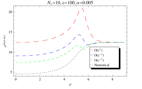
It is easy to see from eq. (12) and the BPS equations eq. (10) that $\mu(c,\alpha)$ is related to the value of the dilaton at $\rho=0$ (see also Fig. 1), namely

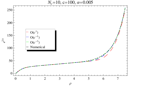
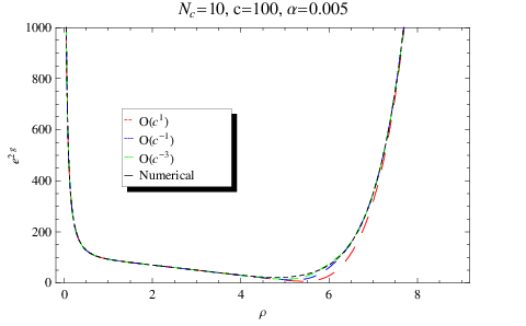
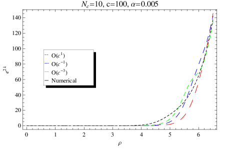
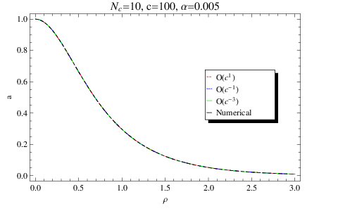
Numerical calculations show that this is indeed a very good approximation. For the UV (large $\rho$) expansions, we refer the reader to the Class II asymptotics in Section 4.3.1 of the paper [29]. Plots of the background functions as functions of $\rho$ are shown in Figs. 1, 2.

The next step is to identify the 4-d physical quantities and to relate them to the background. For example, defining the gauge coupling and its running with energy. In this section we comment on one aspect of this problem.

It will be convenient in this section to reinstate the factors of $\alpha^{\prime}$ and $g_{s}$. Let us start by reminding the reader that the six-dimensional theory on the D5 branes has a ’t Hooft coupling given by $\lambda_{6}=g_{s}\alpha^{\prime}N_{c}$. This coupling has units of length squared as a 6-d coupling should. Now, when we wrap the branes on a small two-cycle $\Sigma_{2}$ and explore the theory at low energies, we will effectively observe a 4-d theory. A natural way of defining the (dimensionless) gauge coupling of this theory is by combining,

Then, the question is how to select the cycle $\Sigma_{2}$. It can be shown that the two-manifold defined by the surface

with the other coordinates $x^{\mu},\rho$ taken to be constant, defines the only two-cycle in the geometry of eq.(6)¹¹ 1 Actually, there is another possible two cycle, given by $\Sigma_{2}^{\prime}=[\theta=\pi-\tilde{\theta},\;\varphi=\tilde{\varphi}\;\;\psi=\pi]$, but this one will give the same results for all the observables we consider here. Probably it is the same two-cycle, with a different orientation.. The characteristic of the submanifold in eq.(29) is that it gets rid of the ‘fibration terms’. In turn, this means that this is the only dimension-2 manifold (without boundaries) that the branes can wrap.

A good definition of the 4-d coupling can be obtained following the papers [31] that considered a “probe” five brane extended along the Minkowski directions and the two-cycle of eq.(29) $R^{1,3}\times\Sigma_{2}$ in the background eq. (6).

The authors of [31] turn on a gauge field $F_{\mu\nu}$ on the Minkowski directions of this five-brane probe (with tension $T_{D5}$) and compute its action (given by the Born-Infeld-Wess-Zumino action);

The induced 6-d configuration on the probe brane extends along $R^{1,3}\times\Sigma_{2}$ is

From here we can compute the determinant²² 2 Notice that the term $\int C_{2,ind}\wedge F_{2}\wedge F_{2}$ will generate the theta-term $\Theta\int d^{4}xF_{\mu\nu}{}^{*}F^{\mu\nu}$. We will omit this term in the following and concentrate on the definition of the gauge coupling.

Plugging this result into eq.(30) and expanding for small values of the field strength (or equivalently, for $\alpha^{\prime}\rightarrow 0$), we get

where we used that $g^{\mu\nu}=e^{-\phi}\eta^{\mu\nu}$. Now, performing the integral over the angles, the term with the Yang-Mills action reads,

From here, and using the fact that the tension of a five brane satisfies $32\pi^{5}g_{s}\alpha^{\prime 3}T_{D5}=1$, we read that the 4-d gauge coupling is

Before we evaluate this quantity on our solution, a few comments are in order.

i) It was shown in the paper [32], that the five branes on the submanifold $R^{1,3}\times\Sigma_{2}$ preserve SUSY only if the probe brane is at infinite radial distance from the end of the space ($\rho\rightarrow\infty$). This result is valid for the particular solution considered there and does not extend to the present background. Indeed, a five brane in the configuration described above does not preserve the same spinors as the background, hence, it is not SUSY, rendering our definition of gauge coupling non SUSY preserving. This will not concern us and we will take the definition of eq.(35) as a good estimation, valid over all the range of the radial coordinate.

ii) If we consider this definition, we can see that the gauge coupling diverges in the IR (signaling confinement). Also, this gauge coupling vanishes in the far UV. The fact that it becomes small should not be a reason of worry. This 4-d gauge being small is not indicating that the ten dimensional geometry is highly curved. Indeed, the 4-d coupling becomes small when the geometry is smooth and well approximated by IIB supergravity.

iii) Using a particular radius-energy relation it was shown in [31] that one particular solution to the eq. of motion (11), reproduces the NSVZ beta function. For the class of solutions we are interested in, the paper [29] shows that the beta function is characteristic of a 6-d field theory.

In Figure 3 we plot the 4-d gauge coupling as defined in eq.(35) on the solutions we found above.

As we have seen above, the gauge coupling exhibits three qualitatively different regimes. Namely, the IR regime for $0<\rho\lesssim 1$, an intermediate plateau for $1\lesssim\rho\lesssim\rho_{*}$ where the gauge coupling is almost constant, and a UV regime for $\rho\gtrsim\rho_{*}$. We study the (approximate) symmetries of the background in these three different regimes.

To leading order in $c/N_{c}$, i.e. in the approximation of eq. (16), the background of eq.(6)-using the definitions in eq.(9)-takes the form

where $d\Omega_{2}^{2}=\omega_{1}^{2}+\omega_{2}^{2}=d\theta^{2}+\sin^{2}\theta d\varphi^{2}$ and $d\tilde{\Omega}_{2}^{2}=\tilde{\omega}_{1}^{2}+\tilde{\omega}_{2}^{2}=d\tilde{\theta}^{2}+\sin^{2}\tilde{\theta}d\tilde{\varphi}^{2}$ are the metrics on two 2-spheres, and we have introduced the one-forms

in addition to the left-invariant $SU(2)$ forms of eq. (3). Let us now look at the behavior of this background in the three different dynamical regimes.

Starting with the far IR, $\rho\lesssim 1$, we see from Table 2 that no further simplifications occur in the above background and so the only isometries are the obvious $ISO(1,3)\times U(1)\times U(1)\times\mathbb{Z}_{2}$, being the two $U(1)^{\prime}s$ the traslations in $\varphi,\tilde{\varphi}$, while $\mathbb{Z}_{2}$ comes from the change $\psi\rightarrow\psi+2\pi$.

In the intermediate regime, $1\lesssim\rho\lesssim\rho_{*}$, we see that the background simplifies to

Note that since $\rho<\rho_{*}$ in this regime we have $\tan^{3}\alpha e^{4\rho}/2<1$. If this was equal to $1$ then the compact part of the metric would be that of $T_{11}$, the base of the conifold. This indeed happens in the UV region, $\rho\gtrsim\rho_{*}$, where the background takes the form