Thermal rectification in nonlinear quantum circuits

Heat transport in nanoscale structures has become an active and rapidly growing research area. Progress in experimental methods has enabled the study of fundamental issues, and lately the field has seen major breakthroughs, such as the measurement of quantized heat transport, [1] and manipulation of thermal currents using external control fields. [2, 3] In solid-state systems electron–electron and electron–phonon scattering are the most important channels for small systems to exchange energy with the environment. However, recently it was understood that at low temperatures one needs to take into account the radiative channel which becomes the dominant relaxation method in mesoscopic samples below the phonon–photon crossover. [2, 4, 5]

In this paper we study rectification effects in thermal transport mediated by electromagnetic fluctuations in solid-state nanostructures. In a two-terminal geometry a finite rectification means that heat current is not simply reversed when the thermal gradient changes sign, but also the absolute magnitude of the current changes. We define the rectification $\cal R$ as

where $J_{+}$ and $J_{-}$ are the magnitudes of the heat currents in forward and reverse bias configurations, respectively (see Fig. 1). Previously rectification has been shown to take place in systems where a classical [6, 7, 8] or quantized [9, 10] nonlinear chain is coupled asymmetrically to linear reservoirs, when nonlinear reservoirs are coupled through a harmonic oscillator, [11] or in hybrid quantum junctions.[12] Here we demonstrate rectification in a fully quantum-mechanical and experimentally realizable model where photon-mediated heat current flows between two linear reservoirs coupled asymmetrically to a nonlinear resonator.

Our analysis is based on a nonequilibrium Green’s function method developed in Ref. 15, and the nonlinear transport problem is solved with a self-consistent Hartree approximation. Rectification is studied as a function of the operating temperatures, reservoir coupling strengths and admittances, and the strength of the nonlinearity. We also propose a concrete setup based on a superconducting quantum interference device (SQUID) where the rectification effects can be realized with current experimental technology at sub-Kelvin temperatures. A similar circuit, operated in the linear regime, was employed in the pioneering experiment demonstrating photonic heat transport. [2] By adjusting the external magnetic flux through the circuit it is possible to tune the rectification continuously between zero and the maximum value. Using realistic parameters we find a rectification of over 10%, and identify a regime where $\cal R$ changes sign as a function of temperature. Experimentally rectification has been observed in phonon transport through a nanotube[13] at room temperature with ${\cal R}=7\%$ and in electron transport through a quantum dot[14] at 80 mK with $\cal R$ up to 10%.

The thermal transport setup is depicted in Fig. 1. It consists of two linear reservoir circuits with admittances $Y_{L}(\omega)$ and $Y_{R}(\omega)$. Temperatures of the left and right reservoirs are $T_{\rm high}$ and $T_{\rm low}<T_{\rm high}$ in the forward bias setting, and vice versa for reverse bias. We assume that heat can flow between the reservoirs only through a mediating nonlinear resonator circuit. The couplings between the reservoirs and the resonator are taken to be inductive with mutual inductances $M_{L}$ and $M_{R}$. Using the Caldeira–Leggett mapping between linear admittances and bosonic reservoir modes the total Hamiltonian takes the form $H=H_{L}+H_{R}+H_{M}+H_{C}$, where the middle circuit and reservoir terms are

and the inductive coupling term is

which involves the current operators for the central device $\hat{I}$ and for the reservoirs $\hat{i}_{L/R}=\sum_{j\in L/R}g_{j}(\hat{a}_{j}+\hat{a}_{j}^{\dagger})$, respectively. The electric current operator for the central device can be expressed as $\hat{I}=I_{0}(\hat{b}+\hat{b}^{\dagger})$ with $I_{0}=\sqrt{\hbar\omega_{0}/2L}$ and $\omega_{0}=1/\sqrt{LC}$ where $L$ and $C$ are the linear inductance and capacitance of the resonator; $\hat{b}$, $\hat{b}^{\dagger}$ and reservoir operators are bosonic creation and annihilation operators, $[\hat{b},\hat{b}^{\dagger}]=1$. The nonlinearity of the central circuit is characterized by the the second term in Eq. (2), corresponding to a quartic potential whose strength is controlled by the parameter $\epsilon$. It must be emphasized that Eq. (4) has a generic bilinear form and therefore our results are relevant for other types of systems beyond the studied realization.

The basis of our analysis is provided by the Meir–Wingreen formula for the heat current [15, 16]

Here $n_{L}(\omega)$ is the Bose function of the left reservoir and $S_{I}(\omega)=\int_{-\infty}^{\infty}dt\,e^{i\omega(t-t^{\prime})}\langle\hat{I}(t)\hat{I}(t^{\prime})\rangle$ is the current noise power of the central circuit. The admittances $Y_{L/R}(\omega)$ are related to the current correlation functions of the free reservoirs. [15] In the absence of the nonlinear term $(\epsilon=0)$ the transport problem can be solved exactly for arbitrary couplings and reservoir admittances. [15] No rectification takes place in this regime. In the following we solve the nonlinear transport problem in a self-consistent Hartree approximation, which is expected to be accurate for small values of the nonlinearity. This approach does not fully account for the correlation effects due to the interplay of nonlinearity and tunneling which are potentially important in the ultra-low temperature regime $T_{\rm high},\,T_{\rm low}\ll\hbar\omega_{0}/k_{B}$. However, analogously to interacting electron transport problems, the mean-field approach is accurate in the sequential tunneling regime when the temperatures are of the order of $\hbar\omega_{0}/k_{B}$.

As a first step we approximate the resonator Hamiltonian as

where we have used $(\hat{b}^{\dagger}+\hat{b})^{4}\approx 6\Phi(\hat{b}^{\dagger}+\hat{b})^{2}$ with the mean field $\Phi=\langle(\hat{b}^{\dagger}+\hat{b})^{2}\rangle$. Here the factor 6 is the number ways two operators can be picked from a set of four. By performing a diagrammatic expansion of the resonator Green’s function one can show that this procedure is identical to the self-consistent Hartree approximation. Because Eq. (6) is now quadratic in bosonic operators, it is possible to bring it to diagonal form by a canonical transformation. However, now we have the added complication of an a priori unknown mean field, which has to be evaluated self-consistently in a nonequilibrium state. The transformed Hamiltonian and current operators are

where $\tilde{\omega}_{0}=\omega_{0}\sqrt{1+\frac{12\epsilon\Phi}{\omega_{0}}}$ and $\tilde{I}_{0}=\sqrt{\frac{\omega_{0}}{\tilde{\omega}_{0}}}I_{0}$. Thus the effect of the nonlinear term is incorporated by a mean-field dependent renormalization of the resonance frequency of the oscillator and its current operator. For further development it is convenient to introduce the correlation functions $\langle\hat{I}(t)\hat{I}(t^{\prime})\rangle^{r}=-i\theta(t-t^{\prime})\langle[\hat{I}(t),\hat{I}(t^{\prime})]\rangle$ and $\langle\hat{I}(t)\hat{I}(t^{\prime})\rangle^{<}=-i\langle\hat{I}(t^{\prime})\hat{I}(t)\rangle$. A nonequilibrium equation-of-motion analysis [18], similar to the one presented in Ref. 15, reveals that the current correlators are given by

where $\langle\hat{I}\hat{I}\rangle^{r}_{0}(\omega)=2\tilde{I}_{0}^{2}\tilde{\omega}_{0}/(\omega^{2}-\tilde{\omega}_{0}^{2})$ is the retarded Green’s function of the uncoupled oscillator. The self-energies

take into account the presence of reservoirs. Furthermore, the mean field $\Phi$ is related to the lesser correlator via

Equations (8)–(12) form a closed set of equations which needs to be solved to find the current correlation functions. The self-consistent solution proceeds by making an initial guess for the mean field, calculating the correlation function $(\ref{iiless})$ corresponding to the initial value and calculating the updated value of the mean field by evaluating the integral in Eq. (12). The procedure is repeated until convergence is achieved. The current noise then follows immediately from the lesser function $S_{I}(\omega)=-\mathrm{Im}\langle\hat{I}\hat{I}\rangle^{<}(-\omega)$ which yields the heat current after evaluating Eq. (5). In the case of a vanishing nonlinearity $(\epsilon=0)$ this procedure recovers the exact solution of the linear problem. To facilitate the analysis of the rectifying mechanism we note that with the help of Eqs. (8)–(12) we can write Eq. (5) in the form

where $F(\omega)=\hbar(\omega^{2}-\omega_{0}^{2}-12\omega_{0}\epsilon\Phi)/(2I_{0}^{2}\omega_{0})$. The frequency dependence of $Y_{L/R}(\omega)$ and $n_{L/R}(\omega)$ has been suppressed for brevity.

For numerical calculations explicit expressions for the admittances $Y_{L/R}(\omega)$ are needed. Here we assume that the reservoir circuits effectively consist of a resistor, a capacitor, and an inductor in series, resulting in $Y_{L/R}(\omega)=R_{L/R}^{-1}[1-iQ_{L/R}(\frac{\omega}{\omega_{L/R}}-\frac{\omega_{L/R}}{\omega})]^{-1}$, where $R_{L/R}$, $Q_{L/R}$, and $\omega_{L/R}$ are the resistance, quality factor and resonance frequency of the left and right reservoir, respectively. The behavior of the system is now uniquely determined by nine dimensionless parameters: $\epsilon/\omega_{0}$, $k_{B}T_{{\rm low}/{\rm high}}/\hbar\omega_{0}$, $M_{L/R}^{2}I_{0}^{2}/\hbar R_{L/R}$, $Q_{L/R}$, and $\omega_{L/R}/\omega_{0}$. Rectification can then be calculated from Eq. (1), by computing the forward and reverse bias currents, $J_{+/-}$, with the above prescription.

Let us illustrate some generic features of the model with the simple setup of two purely dissipative reservoirs, $Q_{L}=Q_{R}=0$, in which case the frequencies $\omega_{L}$ and $\omega_{R}$ are irrelevant. In Fig. 2 we plot the rectification against three different variables. First, from Fig. 2(a) we see that already at quite small values of nonlinearity, $\epsilon\sim 0.1\,\omega_{0}$, the rectification has essentially reached its maximum. Such values for $\epsilon$ are well within the regime of validity of our approximations and should also be easily achieved in the experimental setup proposed below. Next, Fig. 2(b) exemplifies a very generic feature: having $M_{L}^{2}/R_{L}<M_{R}^{2}/R_{R}$ tends to produce $J_{+}>J_{-}$, and vice versa. Finally Fig. 2(c) shows that the rectification increases logarithmically with the temperature ratio $T_{\rm high}/T_{\rm low}$. Therefore, to see an appreciable effect, the temperature difference $T_{\rm high}-T_{\rm low}$ should be of the same order of magnitude as the temperatures themselves.

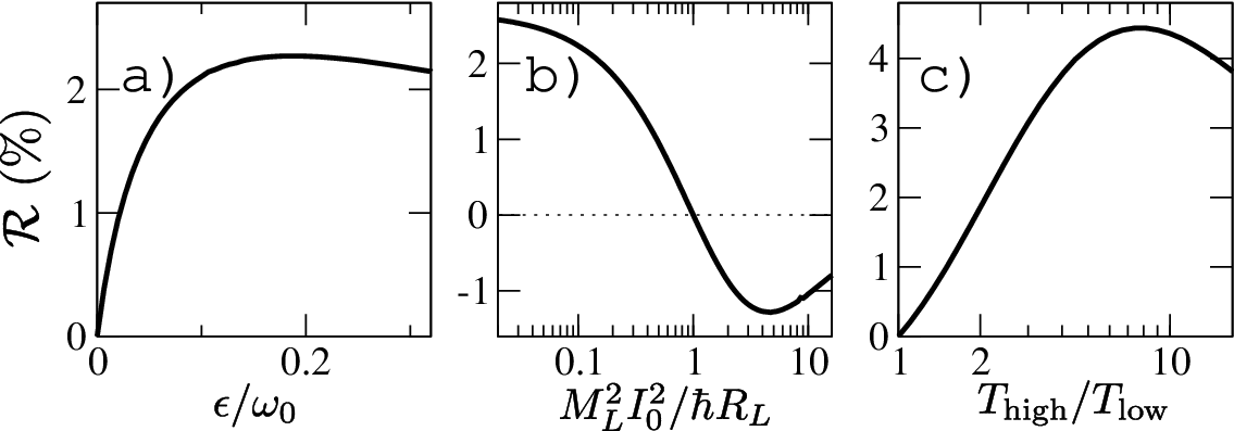
For purely resistive reservoirs maximal value for the rectification is about 2% (Fig. 2(a)). Larger values can be obtained by adding a reactive part to one of the reservoir circuits. Then, as Fig. 3 shows, $\cal R$ can be made an order of magnitude higher. The inset shows the current $J_{+}$, normalized with respect to the universal single-channel maximum heat current $J_{\rm max}=\frac{\pi k_{B}^{2}}{3\hbar}(T_{\rm high}^{2}-T_{\rm low}^{2})$. [17] According to Fig. 3, the highest values for $\cal R$ are obtained for high temperatures, where $J_{+}$ tends to zero. High rectification and large current are thus competing effects, and the optimal operating point depends on the experimental constraints. In any case, it is possible to obtain a rectification of $\sim 5\%$ with $J\sim 0.1\,J_{\rm max}$ and up to $\sim 15\%$ with $J\sim 0.01\,J_{\rm max}$.

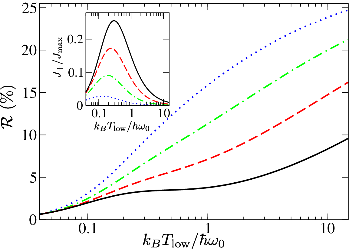
From Fig. 3 we also see that decreasing $\omega_{L}$ increases rectification, so both small $\omega_{L}$ and the condition $M_{L}^{2}/R_{L}<M_{R}^{2}/R_{R}$ favor the direction $J_{+}>J_{-}$. We can also combine these two trends in an opposing manner by making $\omega_{L}$ large. This way one can produce a system where the direction of rectification changes as a function of temperature. From Fig. 4 we see that in a system with a high-frequency reservoir (here $\omega_{L}=10\,\omega_{0}$), ${\cal R}$ is positive when both temperatures are below $\hbar\omega_{0}/k_{B}$, but at higher temperatures the same device produces a negative ${\cal R}$. In contrast to previous reports[8, 19] on the rectification sign reversal, in our system only the reservoir temperatures need to be changed, not the device parameters.

The direction of rectification can be understood as follows. Equations (9) and (12) show that the mean field $\Phi$ is proportional to the self-energy $\Sigma^{<}$. Due to the self-consistency loop the relationship between $\Phi$ and $\Sigma^{<}$ is not actually linear, but in practice making $\Sigma^{<}$ larger will also increase $\Phi$. Next, Eq. (11) shows that $\Sigma^{<}$ is essentially the product of Bose function $n_{L/R}(\omega)$ and the effective coupling strength $\omega M_{L/R}^{2}{\rm Re}[Y_{L/R}({\omega})]$, summed over the two reservoirs. Because of this form, it follows that when comparing the forward and reverse bias settings, larger $\Sigma^{<}$ is obtained in the case when the more strongly coupled reservoir is hotter. As a consequence, the mean field $\Phi$ is also larger when the more strongly coupled reservoir is hotter.

To interpret physically the $\Phi$-dependence of the current $J$, we analyze separately the numerator and denominator of the integrand in Eq. (13). The numerator is the product of the energy $\hbar\omega$, Bose window $n_{L}(\omega)-n_{R}(\omega)$, and effective reservoir coupling strengths, as defined above. Thus it can be seen as a measure of the energy available for transport at the reservoirs. On the other hand, the denominator is due to the Green’s function $|\langle\hat{I}\hat{I}\rangle^{r}(\omega)|^{2}$, giving the transmittance of the central circuit. Equation (13) shows that an increasing $\Phi$ effectively increases the central circuit resonance frequency, thereby shifting the resonator transmission window to higher energies. Because of the Bose functions, in most situations the numerator is smaller at higher energies and the total current decreases. But this is not always the case. It turns out that if at least one of the reservoirs is reactive with high resonance frequency ($\gtrsim\omega_{0}$) and the reservoir temperatures are high ($\gtrsim\hbar\omega_{0}/k_{B}$), the peak of the numerator is shifted to high enough energies so that an increasing $\Phi$ produces on increasing $J$. In summary, except for the case of high-temperature and high-frequency reservoirs, larger current is obtained in the configuration where the more weakly coupled reservoir is hotter. This explains the sign of ${\cal R}$ in all our results.

For low operating temperatures, with $T_{\rm high}$, $T_{\rm low}$ approximately in the range 100 mK–1 K, the studied model can be realized by the setup shown in Fig. 5. The system consists of a superconducting loop containing a Josephson junction characterized by its Josephson energy $E_{J}$ and shunt capacitance $C$. The loop itself is assumed to have a finite inductance dominating the potential landscape. The Hamiltonian of the system is [20]

where the charging and inductive energies are $E_{C}=e^{2}/2C$, $E_{L}=(\hbar/2e)^{2}/2L$, and $\phi_{x}$ denotes the external magnetic flux through the loop (in units of $\hbar/2e$). The superconducting phase across the junction $\hat{\phi}$ and the charge at the capacitor $\hat{q}$ (in units of electron charge) are treated as conjugate observables $[\hat{\phi},\hat{q}]=2i$. The charging term can be thought of as the kinetic energy and the $\phi$-dependent terms as an effective potential energy of a fictitious particle. In the following we assume that $\phi_{x}\approx\pi$ and $E_{J}<2E_{L}$ so that the potential has a single minimum at $\hat{\phi}=\phi_{0}$, with $\phi_{0}\approx\pi$. With these assumptions the phase is bound close to the minimum so that we can approximate the potential accurately by expanding the cosine term to the 4th order:

the second line defining the quantities $E_{2}$ and $E_{4}$. In general there should also be a $\hat{\phi}^{3}$ term, but with $\phi_{0}\approx\pi$ this is small. Further, within the mean-field approximation one has $\hat{\phi}^{3}\sim\hat{\phi}\langle\hat{\phi}^{2}\rangle$, producing just a shift in the origin. Writing the charge and phase in terms of bosonic creation and annihilation operators we recover exactly Eq. (2) with parameters $\hbar\omega_{0}=4\sqrt{E_{C}E_{2}}$ and $\hbar\epsilon=2\frac{E_{C}E_{4}}{E_{2}}$. The current operator of the circuit is given by $\hat{I}=I_{0}(\hat{b}+\hat{b}^{\dagger})$, where $I_{0}=4e(E_{C}E_{2}^{3})^{1/4}/\hbar$. Thus, in the parameter regime $E_{2}\gg E_{4}$ we have effectively realized our weakly nonlinear resonator model.

As the above considerations show, varying the externally applied field $\phi_{x}$ about $\pi$ moves the potential minimum $\phi_{0}$ which in turn changes the values of the parameters $\omega_{0}$ and $\epsilon$. In particular, $\epsilon$ is maximized at $\phi_{x}=\phi_{0}=\pi$ and vanishes when $\phi_{0}\to\pi\pm\pi/2$. Figure 5 demonstrates the resulting continuous tuning of rectification performance.

In conclusion, we have analyzed heat rectification effects in radiative heat transport through a nonlinear quantum resonator. This system is particularly interesting because it can be realized by an experimentally feasible superconducting circuit. The proposed system is operated in a low-temperature regime and can be controlled by by applying external magnetic fields. Despite its simplicity, the system is capable of producing a rectification of over 10%. We have shown that in a suitable parameter regime the direction of rectification changes as a function of temperature and given a physical explanation for the phenomena.

References

- [1] K. Schwab, E. A. Henriksen, J. M. Worlock, and M. L. Roukes, Nature (London) 404, 974 (2000).
- [2] M. Meschke, W. Guichard, and J. P. Pekola, Nature 444, 187 (2006).
- [3] O.-P. Saira et al., Phys. Rev. Lett. 99, 027203 (2007).
- [4] D. R. Schmidt, R. J. Schoelkopf, and A. N. Cleland, Phys. Rev. Lett. 93, 045901 (2004).
- [5] T. Ojanen and T. T. Heikkilä, Phys. Rev. B 76, 073414 (2007).
- [6] M. Terraneo, M. Peyrard and G. Casati , Phys. Rev. Lett. 88, 094302 (2002).
- [7] B. Li, L. Wang and G. Casati, Phys. Rev. Lett. 93, 184301 (2004).
- [8] Bambi Hu, Lei Yang, and Yong Zhang, Phys. Rev. Lett. 97, 124302 (2006).
- [9] D. Segal and A. Nitzan, Phys. Rev. Lett. 94, 034301 (2005).
- [10] N. Zeng and J.-S. Wang, Phys. Rev. B 78, 024305 (2008).
- [11] D. Segal, Phys. Rev. Lett. 100, 105901 (2008).
- [12] L.-A. Wu and D. Segal, Phys. Rev. Lett. 102, 095503 (2009).
- [13] C. W. Chang, D. Okawa, A. Majumdar and A. Zettl, Science 314, 1121 (2006).
- [14] R. Scheibner, M. König, D. Reuter, A. D. Wieck, C. Gould, H. Buhmann, and L. W. Molenkamp, New J. Phys. 10, 083016 (2008).
- [15] T. Ojanen and A.-P Jauho, Phys. Rev. Lett. 100, 155902 (2008).
- [16] In Eq. (5) heat current is positive when energy flows from left to right. Equation (13) in Ref. 15 has an erroneous sign.
- [17] J. B. Pendry, J. Phys. A: Math. Gen. 16, 2161 (1983).
- [18] H. Haug and A.-P. Jauho, Quantum Kinetics in Transport and Optics of Semiconductors (Springer-Verlag, Berlin Heidelberg, 1996).
- [19] D. Segal and A. Nitzan, J. Chem. Phys. 122, 194704 (2005).
- [20] Yu. Makhlin, G. Schön, A. Shnirman, Rev. Mod. Phys. 73, 357 (1999).