Tightened Lieb-Oxford bound for systems of fixed particle number
Abstract
The Lieb-Oxford bound is a constraint upon approximate exchange-correlation functionals. We explore a non-empirical tightening of that bound in both universal and electron-number-dependent form. The test functional is PBE. Regarding both atomization energies (slightly worsened) and bond lengths (slightly bettered), we find the PBE functional to be remarkably insensitive to the value of the Lieb-Oxford bound. This both rationalizes the use of the original Lieb-Oxford constant in PBE and suggests that enhancement factors more sensitive to sharpened constraints await discovery.
I Background
Construction of approximate exchange-correlation (XC) functionals in DFT without reliance on empirical data is an important task, both conceptually and practically. Perhaps the most widely used constraint-based approximate XC functional today is the extremely popular Perdew-Burke-Ernzerhof (PBE) generalized gradient approximation (GGA)[3]. One of the constraints on which the PBE GGA X functional (and some others also) is based is the Lieb-Oxford bound [5]. In the DFT literature this bound commonly is expressed as
| (1) |
where
| (2) |
The LO value for the constant is
| (3) |
The possibility of tightening this bound has been the subject of recurrent interest in DFT. A slightly tighter value was found by Chan and Handy [6]. Vela [7] later reported that using a spatially varying implementation of the LO bound which always is tighter than improved the results for a test set of light inorganic and organic omolecules calculated using constraint-based GGAs.
Shortly thereafter and independently, two of us (OC hereafter) [8, 9] gave numerical evidence from exact and near-exact calculations on atoms, small molecules, and model systems that the true bound is much tighter. That analysis proceeded by defining the functional
| (4) |
with both numerator and denominator evaluated on the actual density of each system. In general, this functional cannot be evaluated exactly, because neither nor the density is known exactly. However, it can be evaluated to high accuracy for systems for which near-exact XC energies and system densities are known from configuration interaction or quantum monte carlo calculations. The result [8, 9] is that real systems typically have . The higher end of the interval typically corresponds to more rarefied, diffuse density distributions, while the lower end corresponds to more compact densities. Values above were only found for extreme low-density limits of model Hamiltonians: the limit of Hooke’s atom has , and the limit of the homogeneous electron gas has .
On the basis of these results, OC conjectured [8, 9] that further tightening of the LO bound, beyond that obtained by Chan and Handy, can be achieved, and suggested that for real systems (excluding unphysical limits of model Hamiltonians) may provide the tightest upper limit, whereas for arbitrary systems is the upper limit.
OC also speculated that system-specific upper limits could be found, thereby providing upper limits for all systems sharing some common properties. Earlier there was other evidence for system-specific limits. Novikov et al. [10] used a reduced parameter (defined below) in the PBE XC functional to some benefit. This reduction (see our discussion below) is equivalent to a reduced LO bound. The numerical rationalization for this was published somewhat later by Peltzer y Blanca et al. [11]. Translating to effective values of , broadly they found that 3d metals do better with , 4d metals benefit from , and 5d metals benefit from . The notable exception was Fe, where the effective was 2.8, an illustration of the fact that all the limitations of a specified XC form cannot be corrected by a single parameter fix. (Recently there also has been study of reduced in the PBE functional but the reduction is done in such a way as to respect the original Lieb-Oxford bound [12], hence is not directly related to the issue at hand.)
Other than this one empirical example, the available data did not allow any general characterization of -value classes. Here we propose and explore a generally applicable, entirely non-empirical way to characterize classes of systems with a common maximum value of . This characterization is based on a rarely mentioned part of the original Lieb-Oxford paper, in which they show that tighter estimates of the upper limit on can be achieved by restricting the functional to densities which integrate to a specified particle number . We therefore introduce the function , which for a given value of provides a universal upper limit upon valid for all systems such that . The maximum value of , attained for , is the value used in common density functionals. The function assigns to each class of systems of common particle number an upper limit .
In construction of constraint-based functionals, the fact that the upper limit can be tightened globally (from to and perhaps on to ) or in a system-specific way (e.g., using ) has not been taken into account, and the consequences of a replacement of by one of the lower values in currently popular functionals are unknown. We study some of those consequences here.
II Construction of a particle-number dependent bound
To explore the system-specific bound provided by the function
requires facing the problem that, while Lieb
and Oxford proved the
existence of this function and deduced some of its properties, they
did not obtain a closed analytical expression for all . We thus
propose a simple approximation to , compatible with all
known information on the universal LO bound. The following
facts are known about [5, 8, 9]:
(i) Its value at is .
(ii) Its value at is not known, but is above
.
(iii) The function is monotonic, i.e.,
.
(iv) Its value at is not known, but must be less than or equal to
. Different proposals for
the value of are , ,
and .
(v) The largest value of found for any system studied
specifically is that for the extreme low-density limit of the
homogeneous electron gas . For
real physical systems, typically . These
values provide empirical lower bounds on the function .
Note that standard density functionals either do not make use of the Lieb-Oxford bound at all (and some are known to violate it [13, 14, 15, 16]) or exploit only property (iv), normally with the weakest value for , namely . To construct a model for the function we exploit properties (i) (value at ), (iii) (monotonicity) and (iv) (value at ). We use properties (ii) (theoretical lower limit at ) and (v) ( for model and real systems) as consistency tests for the construction. With all this in mind, we propose the simple interpolation
| (5) |
where is , or . By construction this interpolation obeys properties (i), (iii) and (iv). Direct inspection shows that it also respects properties (ii) and (v).
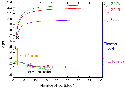
Figure 1 illustrates this function for the three different choices of , and compares it to the known value at , the lower limit at , and some representative data for atoms, molecules, and the homogeneous electron gas.
III Implementation and Computational Protocols
III.1 Modification of PBE GGA
To explore these ideas we have implemented the various possible replacements of in the PBE GGA. At the outset, we remark that, on the basis of previous experience with the revPBE functional [16], we expect that lowering of in PBE will have a detrimental effect on atomic total energies. (In revPBE an increase of was shown to improve atomic total energies and molecular atomization energies, at the expense of worsened bond lengths.)
Since the actual values of for physical systems are known to fall far below , and the theoretical information available from the CH numerical tightening and from the function both indicate that lower values of are appropriate, this detrimental effect must be considered a severe shortcoming of the GGA. An important issue of energetics, therefore, is whether the atomization energies are improved when tightened LO bounds are used in a GGA. (Further investigation is needed to see if meta-GGA functionals [4] suffer from the same problem, but that is beyond the scope of this study.)
In any event, there are five possibilities for tightening, pertaining to two categories. Category I is a simple replacement of the constant value by the alternative lower constants or . Category II replaces the constant by the function , with the three possible choices for . The resulting five choices are to be compared to the original choice , made in the construction of PBE.
In the PBE GGA, the LO bound is enforced pointwise through the choice of the parameter in the exchange enhancement factor
| (6) |
with the dimensionless reduced gradient given by
| (7) |
Taking spin-polarization into account, satisfaction of Eq. (2) by the enhancement factor (6) is equivalent to
| (8) |
Since , the result is
| (9) |
Of course, the simple choice of a different universal bound leads to
| (10) |
The equivalent modification to include the -dependent LO bound, Eq. (5), is
| (11) |
The result of considering such altered LO bounds is five variants of
the PBE X functional:
PBEMA: PBE96 X but with .
PBEMB: PBE96 X but with .
PBEMC: PBE96 X but with and .
PBEMD: PBE96 X but with and
.
PBEME: PBE96 X but with
and .
The first two, along with the original PBE,
comprise category I, the latter three,
category II. We denote the five variants collectively as PBEMx in
what follows.
III.2 Protocols
All five variants were introduced in the code deMon2k, version 2.4.2 [17], by systematic modification of the exchange-correlation modules. Subsequently, the implementation was validated by comparison of atomic calculations done with hard-coded modifications of the code soatom.f [18]. Throughout we used the full PBE correlation functional, not the deMon cutoff version (i.e. we used the deMon2k “PBESSF” option), both for ordinary PBE and PBEMx. Because deMon2k uses variational Coulomb fitting, there is a choice of density fitting (auxiliary) basis sets and of the method for evaluating XC matrix elements. Initially we used the so-called A2 density fitting basis (deMon2k option AUXIS(2)) and the option to do the numerical integrals for the XC quantities using the fitted (auxiliary) density (deMon2k “AUXIS” option). We return to these options below.
For development of a suitable protocol (Kohn-Sham basis, fitting basis) we first studied the Li2 molecule in a triple-zeta-plus-polarization (TZVP) KS basis. The results are in Table 1. Note that is the total atomization energy, (not the cohesive energy per atom). Regarding the quality of the calculation, observe that for the unmodified PBE functional, our results are almost identical with those given by Ernzerhof and Scuseria [19], kcal/mol, Å. (For reference, they quote experimental values as kcal/mol and Å.)
As would be expected from naïve use of a particle-number-dependent model, the results in Table 1 show a clear size-inconsistency problem, signaled by the big shift in between the -independent models, PBE, PBEMA, PBEMB, and the -dependent models, PBEMC, PBEMD, and PBEME. The fact that there is no such shift in the values is a clear sign that the problem is in the comparison with the isolated atom. Eq. (11) illustrates the point. In a naïve application of the -dependent models, the Li atom has while the Li2 molecule has (with the three choices of ). The result is a separated atom limit of the diatomic molecule which is not the same as the isolated atom. Table 2 shows the very substantial difference in the PBE parameter for these two situations.
| Functional | ||||
|---|---|---|---|---|
| PBE | -7.460992748 | -14.953949056 | 20.06 | 2.7236 |
| PBEMA | -7.457436406 | -14.946932892 | 20.01 | 2.7218 |
| PBEMB | -7.441633876 | -14.915640294 | 20.31 | 2.7155 |
| PBEMC | -7.442385785 | -14.937217688 | 32.91 | 2.7196 |
| PBEMD | -7.439006265 | -14.930264047 | 32.79 | 2.7181 |
| PBEME | -7.424518016 | -14.899876726 | 31.90 | 2.7131 |
| Functional | ||
|---|---|---|
| PBE | 0.804319 | 0.804319 |
| PBEMA | 0.757967 | 0.757967 |
| PBEMB | 0.587401 | 0.587401 |
| PBEMC | 0.594439 | 0.699379 |
| PBEMD | 0.563537 | 0.660752 |
| PBEME | 0.449826 | 0.518614 |
| Functional | ||||
|---|---|---|---|---|
| PBE | -7.460992748 | -14.953949056 | 20.06 | 2.7236 |
| PBEMA | -7.457436406 | -14.946932892 | 20.01 | 2.7218 |
| PBEMB | -7.441633876 | -14.915640294 | 20.31 | 2.7155 |
| PBEMC | -7.452520577 | -14.937217688 | 20.19 | 2.7196 |
| PBEMD | -7.449007723 | -14.930264047 | 20.24 | 2.7181 |
| PBEME | -7.433703689 | -14.899876726 | 20.37 | 2.7131 |
| PBE | -7.460613173 | -14.953310471 | 20.13 | 2.7304 |
| PBEMA | -7.457076546 | -14.946319641 | 20.18 | 2.7277 |
| PBEMB | -7.441303732 | -14.915029100 | 20.34 | 2.7181 |
| PBEMC | -7.452179554 | -14.936623118 | 20.25 | 2.7244 |
| PBEMD | -7.448674591 | -14.929672255 | 20.28 | 2.7222 |
| PBEME | -7.433359029 | -14.899212818 | 20.39 | 2.7143 |
| Reference values [20, 21, 22, 23] | -7.47806 | -14.9938 | 26 | 2.673 |
Table 3 shows how a size-consistent set of parameters, here for , resolves the problem. (For clarity, note we made the common choice throughout all these calculations and ignored the DFT spin-symmetry problem. Thus, the separated atoms are spin-polarized even though the molecule has multiplicity equal one.) Throughout this study, we used this same size-consistent procedure, namely applying to the separated atoms the modified LO constants proper for the value of of the aggregated system (molecule) in question. For heteronuclear molecules, especially hydrides, this protocol results in a rather disparate enforcement of the LO bound for atoms of substantially different , a matter for later study and refinement. (We note that the use of the original PBE functional implies the most disparate enforcement of all, as it amounts to using the largest value of for all finite .)
Table 3 also compares the effect of the two different options in deMon2k for evaluation of the XC matrix elements. First is the deMon A2 density fitting basis (deMon2k option AUXIS(2)) and the aforementioned deMon2k option (“AUXIS”) for evaluation of XC quantities using the fitted (auxiliary) density on a numerical grid. Second is the richer GEN-A2 fitting basis and evaluation of the the XC quantities from the density formed straightforwardly from the KS orbitals also on the numerical grid (“BASIS” option). In principle, the latter procedure is the more accurate and is the one we adopted. Nevertheless, the trends in the PBEMx series are essentially the same in the less-accurate procedure.
Our other exploratory test was the O2 molecule, a triplet ground state system. The TZVP PBE atomization energy (see the first two lines of Table 4) is about three percent off from the published result of Ernzerhof and Scuseria [19], who used the substantially richer basis 6311+G(3df,2p). An ACES-II [24] calculation using another rich basis (aug-cc-PVTZ) matched the deMon2k results with that same KS basis and the richer density-fitting basis (“GEN-A2*” option). These results, in the third and fourth lines of Table 4, calibrate the effects of basis set differences. Results for the PBEMx series in the aug-cc-PVTZ/GEN-A2* basis sets also are in Table 5. The relative shifts among the six PBE variants are the same irrespective of basis sets, but the richer basis sets make the atomization energies larger and bond lengths slightly shorter. Ernzerhof and Scuseria [19] quote the experimental data as = 118 kcal/mol and = 1.208 Å. Thus, all six PBE variants (original plus five new give too deep a binding energy at slightly elongated bond lengths.
| Calc. | ||||
|---|---|---|---|---|
| deMon-TZVP | -75.00612438 | -150.23282532 | 138.4 | 1.23491 |
| ES | 143 | 1.217 | ||
| AP | -75.00773627 | -150.24372619 | 143.2 | 1.21996 |
| deMon-aug | - 75.00781596 | -150.24387554 | 143.2 | 1.22008 |
| Functional | ||||
|---|---|---|---|---|
| PBE | -75.00612438 | -150.23282532 | 138.4 | 1.2349 |
| PBEMA | -74.99689680 | -150.21624772 | 139.6 | 1.2343 |
| PBEMB | -74.95432779 | -150.13915494 | 144.6 | 1.2315 |
| PBEMC | -74.99835094 | -150.21886346 | 139.4 | 1.2344 |
| PBEMD | -74.98900193 | -150.20202494 | 140.6 | 1.2338 |
| PBEME | -74.94639261 | -150.12467907 | 145.5 | 1.2310 |
| PBE | -75.00781596 | -150.24387554 | 143.2 | 1.2201 |
| PBEMA | -74.99853463 | -150.22722985 | 144.4 | 1.2195 |
| PBEMB | -74.95571887 | -150.14986185 | 149.6 | 1.2167 |
| PBEMC | -74.99998015 | -150.22985618 | 144.3 | 1.2196 |
| PBEMD | -74.99059055 | -150.21295118 | 145.4 | 1.2189 |
| PBEME | -74.94774275 | -150.13534295 | 150.5 | 1.2162 |
| Reference values [20, 21, 22, 23] | -75.0674 | -150.2770 | 118 | 1.208 |
The preceding discussion makes clear that systematic comparison of the five PBE variants generally does not require a fully saturated basis set. Rare gas dimers, discussed below, are an exception. Therefore, except for rare gas dimers, we adopted the following protocol: (i) use TZVP for the KS basis; (ii) Use GEN-A2 or GEN-A3 algorithms to generate the fitting-function basis (and thereby minimize the effect of the variational Coulomb fitting, which gives a lower bound to the Coulomb repulsion that can be deceptive with a poorly chosen fitting basis); (iii) use the deMon2k BASIS option for evaluation of the XC matrix elements. This protocol combines a reasonably rich KS basis with an abundance of caution in treating the XC quantities.
For the rare gas dimers, test calculations on Ar2 with both a DZVP and a 6-311++G(3df,3pd) KS basis set demonstrated that these do not reproduce known, large-basis PBE results for this dimer [26, 27]. Since those two calculations were completely independent and gave essentially identical values, kcal/mol, Å, it is essential to reproduce them. Therefore, we shifted to the aug-cc-pVTZ KS basis [28], as used by Zhao and Truhlar, and the deMon2k GEN-A3 fitting function basis. This combination gives the same PBE results as the foregoing two references. We treated Ne2 with the corresponding aug-cc-pVTZ KS basis and GEN-A3 fitting function basis.
IV Results and Discussion
For PBE and PBEMx, Table 6 gives the atomization energies for eighteen light molecules, while 7 gives bond lengths and bond angles for those same systems. (As a technical aside, note that NiH is a difficult system to treat.) Absolute relative errors in the atomization energy are shown in Figure 2 and the corresponding bond length data are in Figure 3.


Several features stand out from these results. With a few exceptions, the general pattern is that both atomization energies and bond lengths are remarkably insensitive to changes in the enforcement of the LO bound. This outcome is consistent with what one might have intuited from Figure 1. The which we are justified in using (in the sense that our interpolation respects the known constraints) is substantially larger than the values imputed for actual molecules. So one might conclude that a more refined way of implementing the LO bound in a GGA is needed.
However, two systems, Ne2 and Ar2, are notably sensitive to the value of in the atomization energies. A coherent interpretation by classes of molecules is possible: unlike the other atoms, Ne and Ar are closed shell systems. Thus, we may suspect that the well-known peculiarities of closed shell interactions are the source of the distinct behavior. For the equilibrium bond lengths Ne2 and Ar2 still stand out from all other systems by being most sensitive to changes in . (See Fig. 3.) Interestingly, the Be2 bond-length variation is at odds with all the other open-shell systems. The behavior of Be2 does not seem to be traceable to being from the rapidly varying part of the function, since Li2 is in that region also and it is insensitive in both bond length and atomization energy.


To display the effects of imposition of the size-consistent molecular values on the LO bounds in atoms, we also calculated some isolated atom total energies at their intrinsic values. For H, C, N, O, and F, Table 8 displays the results for the intrinsic value versus the results for the highest molecule in which each element was used in the present study. As would be expected from the interpolation, Eq. (5), and the constraints on which it is based, the total energy of the H atom exhibits the largest percentage variation between intrinsic and molecular values for for the three -dependent variants (PBEMC, PBEMD, PBEME).
| Species | PBE | PBEMA | PBEMB | PBEMC | PBEMD | PBEME | Exp [22] | |
|---|---|---|---|---|---|---|---|---|
| Li2 | 1 | 20.13 | 20.18 | 20.34 | 20.25 | 20.28 | 20.39 | 26 |
| Be2 | 1 | 9.71 | 9.95 | 10.94 | 10.12 | 10.35 | 11.28 | 2.3 |
| B2 | 3 | 76.7 | 77.3 | 80.1 | 77.6 | 78.2 | 80.8 | 71.3 |
| C2 | 1 | 142.3 | 143.4 | 147.9 | 143.6 | 144.6 | 148.9 | 146 |
| N2 | 1 | 235.5 | 236.7 | 241.7 | 236.7 | 237.9 | 242.6 | 227 |
| O2 | 3 | 138.4 | 139.6 | 144.6 | 139.4 | 140.6 | 145.5 | 118 |
| F2 | 1 | 51.56 | 52.46 | 56.30 | 52.23 | 53.12 | 56.90 | 38 |
| Ne2 | 1 | 0.1279 | 0.1438 | 0.2236 | 0.1385 | 0.1549 | 0.2369 | 0.0839 |
| Ar2 | 1 | 0.1377 | 0.1631 | 0.2998 | 0.1462 | 0.1732 | 0.3122 | 0.2846 |
| HF | 1 | 142.645 | 143.161 | 145.401 | 143.356 | 143.864 | 146.037 | 142 |
| LiH | 1 | 54.53 | 54.54 | 54.57 | 54.57 | 54.57 | 54.54 | 58 |
| OH | 2 | 110.361 | 110.762 | 112.458 | 110.976 | 111.365 | 112.981 | 107 |
| NH | 3 | 88.95 | 89.18 | 90.07 | 89.34 | 89.55 | 90.36 | 88 |
| NiH | 2 | 74.05 | 75.05 | 76.63 | 74.86 | 75.21 | 76.79 | 58.8 |
| H2O | 1 | 235.9 | 236.8 | 240.5 | 237.1 | 237.9 | 241.5 | 235 |
| NH3 | 1 | 305.686 | 306.664 | 310.761 | 307.029 | 307.976 | 311.882 | 297 |
| CH4 | 1 | 427.184 | 428.245 | 432.736 | 428.641 | 429.673 | 433.983 | 420 |
| C6H6 | 1 | 1423.74 | 1430.39 | 1458.48 | 1425.84 | 1432.45 | 1460.30 | 1362 |
| Species | PBE | PBEMA | PBEMB | PBEMC | PBEMD | PBEME | Exp [23] |
|---|---|---|---|---|---|---|---|
| Li2 | 2.7304 | 2.7277 | 2.7181 | 2.7244 | 2.7222 | 2.7143 | 2.673 |
| Be2 | 2.4409 | 2.4379 | 2.4259 | 2.4355 | 2.4328 | 2.4218 | 2.45 |
| B2 | 1.6208 | 1.6198 | 1.6159 | 1.6194 | 1.6185 | 1.6148 | 1.590 |
| C2 | 1.2595 | 1.2590 | 1.2567 | 1.2590 | 1.2584 | 1.2562 | 1.243 |
| N2 | 1.1112 | 1.1108 | 1.1091 | 1.1108 | 1.1104 | 1.1087 | 1.098 |
| O2 | 1.2349 | 1.2343 | 1.2315 | 1.2344 | 1.2338 | 1.2310 | 1.208 |
| F2 | 1.4301 | 1.4290 | 1.4242 | 1.4293 | 1.4282 | 1.4235 | 1.412 |
| Ne2 | 3.0808 | 3.0418 | 2.8709 | 3.0546 | 3.0162 | 2.8550 | 3.091 |
| Ar2 | 3.99907 | 3.9124 | 3.6964 | 3.9469 | 3.8929 | 3.6841 | 3.7565 |
| HF | 0.9385 | 0.9385 | 0.9385 | 09385 | 0.9385 | 0.9385 | 0.917 |
| LiH | 1.6065 | 1.6058 | 1.6029 | 1.6039 | 1.6033 | 1.6012 | 1.595 |
| OH | 0.9899 | 0.9899 | 0.9898 | 0.9899 | 0.9899 | 0.9897 | 0.971 |
| NH | 1.0549 | 1.0549 | 1.0548 | 1.0549 | 1.0549 | 1.0548 | 1.036 |
| NiH | 1.4580 | 1.4594 | 1.4553 | 1.4599 | 1.4590 | 1.4549 | 1.477 |
| H2O, R | 0.9750 | 0.9749 | 0.9747 | 0.9749 | 0.9749 | 0.9746 | 0.959 |
| H2O, | 104.21 | 104.24 | 104.39 | 104.25 | 104.29 | 104.43 | 103.9 |
| NH3, R | 1.0252 | 1.0252 | 1.0245 | 1.0250 | 1.0249 | 1.0244 | 1.012 |
| NH3, | 106.40 | 106.44 | 106.62 | 106.45 | 106.49 | 106.67 | 106.7 |
| CH4 | 1.0990 | 1.0989 | 1.0984 | 1.0988 | 1.0987 | 1.0982 | 1.086 |
| C6H6, RCC | 1.3995 | 1.3990 | 1.3965 | 1.3994 | 1.3988 | 1.3963 | 1.397 |
| C6H6, RCH | 1.0947 | 1.0946 | 1.0943 | 1.0947 | 1.0946 | 1.0943 | 1.084 |
| XC | H | C | N | O | F |
|---|---|---|---|---|---|
| PBE | -0.498147969 | -37.794851185 | -54.530389203 | -75.006124382 | -99.664580137 |
| PBEMA | -0.497515476 | -37.787528107 | -54.522145702 | -74.996896796 | -99.654626939 |
| PBEMB | -0.494726517 | -37.754129975 | -54.484419695 | -74.954327792 | -99.608420218 |
| PBEMC | -0.481206885 | -37.777286824 | -54.513676785 | -74.989918352 | -99.649171204 |
| (intrinsic ) | |||||
| PBEMC | -0.497950959 | -37.792580522 | -54..52240237 | -74.99835094 | -99.65716700 |
| (highest ) | |||||
| PBEMD | -0.481206885 | -37.769885027 | -54.505322010 | -74.980521867 | -99.639010126 |
| (intrinsic ) | |||||
| PBEMD | -0.497316032 | -37.785199634 | -54.51406717 | -74.98900193 | -99.64707222 |
| (highest ) | |||||
| PBEME | -0.481206885 | -37.736869483 | -54.467831152 | -74.937949507 | -99.592621018 |
| (intrinsic ) | |||||
| PBEME | -0.494539297 | -37.751826019 | -54.47640949 | -74.94639261 | -99.60074422 |
| (highest ) | |||||
| exact [20] | -0.5 | -37.8450 | -54.5893 | -75.0674 | -99.7341 |
V Concluding Remarks
Our results show that PBE is rather insensitive to changes in for atoms and covalently and ionically bound small molecules. Overall, a reduced, and thus, in principle, better, value of produces slightly worsened energies and slightly improved bond lengths. This insensitivity explains why PBE can be successful even though it uses the value even for small . In this sense, the present study provides additional insight into the success of PBE for small systems. On the other hand, a suitably designed, constraint-based functional should give improved results when the constraints it incorporates are sharpened. The failure of PBE to meet this expectation must be considered a limitation of the PBE functional form.
In the case of the closed shell systems, we find a more pronounced dependence than in the covalent and ionic systems. Because of the delicate nature of binding in these systems, more detailed investigation would be needed to make conclusive statements. In the spirit of the preceding paragraph, it would appear to be more productive to focus on developing enhancement factors that are more sensitive to sharpening of constraints.
An appealing thought is that the insensitivity found here may also have to do with the way that the LO bound is implemented in DFT in general. The original LO bound is for the Coulomb exchange and correlation energy and does not include the correlation kinetic energy, , which contributes to . As a result, and the functional which was evaluated in [8, 9] is smaller than the functional
| (12) |
If the effect of Tc were large enough, it might explain at least part of the large difference between the values of and in Figure 1. What limited numerical evidence we have, however, suggests that is only about 10% larger than , a very modest shift compared to the difference in Figure 1.
The more general point, however, that the LO bound is a constraint on exchange and correlation together, seems to be sustained by our findings, in that the PBE form enforces the bound purely on exchange. One speculation is that the insensitivity found here is in part a consequence of that restricted use of the LO bound.
Finally, we consider aspects of -dependence and chemical classification for enforcement of the LO bound. The first insight is that, in retrospect, -dependent satisfaction of the LO bound actually arose very early in DFT, before the LO proof. In Slater’s X model, is modeled by scaling . (From a modern perspective, X is a one-parameter XC model which gains simplicity at the cost of violating correct scaling for C.) The parameter is -dependent [33] and exhibits very clear shell structure [34, 35]. For X, the LO functional of Eq. (4) is just . With typical values of [34, 35], this gives for H y() to for Rn (). Comparison with Fig. 1 shows that these values are slightly smaller than the highly accurate empirical values found in Refs. [8, 9].
The importance of shell-dependent classification was evident in the modern work of Refs. [8] and [9]. The numerical results of this study also leave a strong suggestion that such classification would be helpful. An advantage of the present classification of with respect to alone is that it can be done in an entirely non-empirical way, as it relies only upon exact properties of the function . (This is a clear distinction from all parameterized approaches.) Of course, the choice of interpolating function is not unique, but the fact that the upper limit on depends on is completely general. So are all the properties of used in the construction of our interpolation. What this means is that whatever shell-dependent classification might be invented, it must somehow be an addition to (or incorporate) classification by particle number, not supplant it. Because that classification will have to avoid size-inconsistency, we suspect that the formulation will require additional insight, including additional constraints.
VI Acknowledgments
SBT thanks Ajith Perera for the ACES-II calculations on O2, and Andreas Köster, Gerald Geudtner, and Patrizia Calaminici (Cinvestav, México DF) for technical advice on the use of deMon2k. MMO was supported by FAPESP. KC was supported by FAPESP and CNPq. SBT was supported in part by the U.S. National Science Foundation under DMR-0325553 (ITR).
References
- [1] J.P. Perdew, in “Electronic Structure of Solids ’91”, P. Ziesche and H. Eschrig eds. (Akademie Verlag, Berlin, 1991) p. 11.
- [2] J.P. Perdew and M. Levy, Phys. Rev. B 48, 11638 (1993).
- [3] J.P. Perdew, K. Burke, and M. Ernzerhof, Phys. Rev. Lett. 77, 3865 (1996); erratum Phys. Rev. Lett. 78, 1396 (1997).
- [4] J.P. Perdew, J. Tao, V.N. Staroverov, and G.E. Scuseria, J. Chem. Phys. 120, 6898 (2004).
- [5] E.H. Lieb and S. Oxford, Int. J. Quantum Chem. 19, 427 (1981); E.H. Lieb, Phys. Lett. 70A, 444 (1979).
- [6] G.K.-L. Chan and N.C. Handy, Phys. Rev. A 59, 3075 (1999).
- [7] “The Lieb-Oxford Bound and the Large Gradient Correction in the Exchange Energy”, Alberto Vela, Symposium 19, XVth Internat. Materials Research Congress, Acad. Méxicana de Ciencía de Materiales, Cancún México, 22 August 2006.
- [8] M.M. Odashima and K. Capelle, J. Chem. Phys. 127, 054106 (2007).
- [9] M.M. Odashima and K. Capelle, Int. J. Quantum Chem. 108, 2428 (2008).
- [10] D.L. Novikov, A.J. Freeman, N.E. Christensen, A. Svane and C.O. Rodriguez, Phys. Rev. B 56, 7206 (1997).
- [11] E.L. Peltzer y Blanca, C.O. Rodriguez, J. Shitu, and D.L. Novikov, J. Phys. Cond. Matt 13, 9463 (2001).
- [12] G.I. Csonka, O.A. Vydrov, G.E. Scuseria, A. Ruzsinszky, and J.P. Perdew, J. Chem. Phys. 126, 244107 (2007).
- [13] J.P. Perdew and Y. Wang, Phys. Rev. B 33, 8800 (1986); ibid. 40, 3399 (1989); J.P. Perdew, Phys. Rev. B. 33, 8822 (1986); ibid. 34, 7406 (1986).
- [14] A.D. Becke, Phys. Rev. A 38, 3098 (1988); C. Lee, W. Yang and R. G. Parr, Phys. Rev. B 37, 785 (1988).
- [15] L.C. Wilson and M. Levy, Phys. Rev. B 41, 12930 (1990).
- [16] Y. Zhang and W. Yang, Phys. Rev. Lett. 80, 890 (1998); J.P. Perdew, K. Burke, and M. Ernzerhof, Phys. Rev. Lett. 80, 891 (1998).
- [17] deMon2K; A.M. Köster, P. Calaminici, M.E. Casida, R. Flores-Moreno, G. Geudtner, A. Goursot, T. Heine, A. Ipatova, F. Janetzco, J. Martin del Campo, S. Patchkovskii, J.U. Reveles, D.R. Salahub, and A. Vela, The deMon Developers, Cinvestav, México DF, México (2006)
- [18] S.B. Trickey, J.A. Alford, and J.C. Boettger, in “Computational Materials Science”, vol. 15 of Theoretical and Computational Chemistry, J. Leszczynski ed. (Elsevier, Amsterdam, 2004)) 171; J.C. Boettger, Phys. Rev. B 62, 7809 (2000), U. Birkenheuer, J.C. Boettger, and N. Rösch, J. Chem. Phys. 100, 6826 (1994); J.C. Boettger, Int. J. Quantum Chem. S27, 147 (1993); J.W. Mintmire, J.R. Sabin, and S.B. Trickey, Phys. Rev. B 26, 1743 (1982).
- [19] M. Ernzerhof and G.E. Scuseria, J. Chem. Phys. 110, 5029-5036 (1999).
- [20] Total atomic energies from E.R. Davidson, S.A. Hagstrom, S.J. Chakravorty, V.M. Umar, and C. Froese Fischer, Phys. Rev. A 44, 7071 (1991); S.J. Chakravorty and E.R. Davidson, J. Phys. Chem. 100, 6167 (1996).
- [21] Diffusion Monte Carlo total energies for , , , , , and from C. Filippi and C. J. Umrigar, J. Chem. Phys. 105, 213 (1996); for LiH, NH, OH and HF from A. Lüchow and J.B. Anderson, J. Chem. Phys. 105, 7573 (1996); for , , , from S. Manten and A. Lüchow, J. Chem. Phys. 115, 5362 (2001); for from M. Casula, C. Attaccalite and S. Sorella, J. Chem. Phys. 121, 7110 (2004).
- [22] Experimental atomization energies for , , , , LiH, NH, OH, HF, , , , from [19]; for from V.E. Bondybey, Chem. Phys. Lett. 109, 436 (1984); for from M.T. Carrol, R.F.W. Bader and S.H. Vosko, J. Phys. B: At.Mol.Phys. 20 3599 (1987); for from A. Goursot, J.P. Malrieu and D.R. Salahub, Theor. Chim. Acta 91, 225 (1995); for and from J.F. Ogilvie and F.Y.H. Wang, Exp J. Mol. Struct. 273, 277 (1992); for NiH from C.V. Diaconu, A.E. Cho, J.D. Doll, and D. L. Freeman, J. Chem. Phys. 121, 10026 (2004);
- [23] Experimental bond lengths for , , , , LiH, NH, OH and HF from [19]; for from V.E. Bondybey, Chem. Phys. Lett. 109, 436 (1984); for from V.N. Staroverov, G.E. Scuseria, J. Tao and J.P. Perdew, J. Chem. Phys. 119, 12129 (2003); for from A. Goursot, J.P. Malrieu and D.R. Salahub, Theor. Chim. Acta 91, 225 (1995); for , and from D. J. DeFrees, B. A. Levi, S. K. Pollack, W. J. Hehre, J. S. Binkley and J. A. Pople, J. Am. Chem. Soc. 101, 4085 (1979); for from D. W. H. Swensona, H. M. Jaegera and C. E. Dykstra, Chem. Phys. 326, 329 (2006); for and from J.F. Ogilvie and F.Y.H. Wang, Exp J. Mol. Struct. 273, 277 (1992); for NiH from C.V. Diaconu, A.E. Cho, J.D. Doll, and D. L. Freeman, J. Chem. Phys. 121, 10026 (2004);
- [24] J.F. Stanton, J. Gauss, S.A. Perera, J.D. Watts, M. Nooijen, A. Yau, N. Oliphant, P.G. Szalay, W.J. Lauderdale, S.R. Gwaltney, S. Beck, A.Balková, D.E. Bernholdt, K.-K. Baeck, P. Rozyczko, H. Sekino, C. Huber, J. Pittner, and R.J. Bartlett; ACES-II, is a program product of the Quantum Theory Project, University of Florida. Integral packages included are VMOL (J. Almlöf and P.R. Taylor); VPROPS (P.R. Taylor); ABACUS (T. Helgaker, H.J.Aa. Jensen, O. Jørgensen, J. Olsen, and P.R. Taylor)
- [25] S.A. Perera, Univ. of Florida, May 2008 [unpublished].
- [26] D.C. Patton and M.R. Pederson Phys. Rev. A 56, R2495 (1997); erratum Phys. Rev. A 71, 019906(E) (2005).
- [27] Y. Zhao and D.G. Truhlar, J. Phys. Chem. A 110, 5121, 2006.
- [28] Extensible Computational Chemistry Environment Basis Set Database, Version 1.0, as developed and distributed by the Molecular Science Computing Facility, Environmental and Molecular Sciences Laboratory which is part of the Pacific Northwest Laboratory, P.O. Box 999, Richland, Washington 99352, USA, and funded by the U.S. Department of Energy. The Pacific Northwest Laboratory is a multi-program laboratory operated by Battelle Memorial Institue for the U.S. Department of Energy under contract DE-AC06-76RLO 1830.
- [29] http://www.ipc.uni-karlsruhe.de/tch/tch1/index.de.html
- [30] I.C. Gerber and J.G. Ángyán, Chem. Phys. Lett. 416, 370 (2005).
- [31] I. Cabria, M.J. López, and J.A. Alonso, Nanotech. 17, 778 (2006).
- [32] A. Becke, J. Chem. Phys. 84, 4524 (1986).
- [33] J.C. Slater, Adv. Quantum Chem. 6, 1 (1972).
- [34] K. Schwarz, Phys. Rev. B 5, 2466 (1972).
- [35] K. Schwarz, Theoret. Chim. Acta 34 225 (1974).