Mesoscopic Spin-Hall Effect in 2D electron systems with smooth boundaries
Abstract
Spin-Hall effect in ballistic 2D electron gas with Rashba-type spin-orbit coupling and smooth edge confinement is studied. We predict that the interplay of semiclassical electron motion and quantum dynamics of spins leads to several distinct features in spin density along the edge that originate from accumulation of turning points from many classical trajectories. Strong peak is found near a point of the vanishing of electron Fermi velocity in the lower spin-split subband. It is followed by a strip of negative spin density that extends until the crossing of the local Fermi energy with the degeneracy point where the two spin subbands intersect. Beyond this crossing there is a wide region of a smooth positive spin density. The total amount of spin accumulated in each of these features exceeds greatly the net spin across the entire edge. The features become more pronounced for shallower boundary potentials, controlled by gating in typical experimental setups.
pacs
73.23.-b, 72.25.-bIntroduction. Spin-Hall effect [2], manifested in the boundary spin polarization when electric current flows through a system with significant spin-orbit interaction, was recently observed in both 3D [3, 4, 5] and 2D systems [6]. Two mechanisms that lead to the effect are typically distinguished. The extrinsic mechanism is dominant in 3D semiconductors and originates from scattering off impurities [7, 8, 9, 10]. Intrinsic mechanism [11, 12] of the band-structure induced spin precession can be realized in ballistic (disorder-free) 2D systems.
The intrinsic spin-Hall mechanism is of particular appeal. However, in two-dimensional electron systems with spin-orbit coupling linear in momentum (typical for -doped heterostructures) any scattering that leads to a stationary electric current via deceleration of electrons by impurities, phonons, etc., will negate the precession due to external electric field and result in the exact cancellation [13, 14, 15, 16, 17] of the bulk spin-current in a dc case [18].
One possible way to avoid this cancellation is to move into the ac domain with frequencies exceeding the inverse spin relaxation time [14]. Another possibility is to use dc fields but make a system sufficiently small and clean (ballistic) so that the electron mean free time exceeds the time of flight across the systems. The corresponding scenario became known as the mesoscopic spin-Hall effect [23]. While initial theories of spin-Hall effect in infinite systems had addressed such auxiliary quantity as spin current (for a review see Refs. [19, 20]), finite geometry calls for calculations of spin polarization, a directly measurable quantity [21].
It is important to emphasize that the edge spin polarization in ballistic systems appears not as a result of electric field-driven acceleration of electrons and associated with it precession of spins. Instead, it originates from their precession in the course of electron motion in the boundary potential that provides lateral confinement. When populations of left- and right-moving states are different (due to the applied bias) the net effect of this precession results in a non-zero spin polarization. Such edge polarization was considered, mostly by numerical methods, in several earlier publications [22, 23, 24, 25, 26].

The total amount of accumulated spin near an edge of a 2DEG is independent of the boundary potential, as found in our recent study [27], yet only second order in the spin-orbit coupling constant. In the present paper we show how to overcome this limitation and achieve a much larger local spin-Hall polarization over extended strips along the edge of 2DEG provided that smooth boundaries are utilized. Increasing the width of the edge by making the boundary potential progressively smoother, one can increase the amount of spin accumulated within each strip. The sign of the polarization in these strips will alternate so that the net spin accumulation will be in agreement with Ref. [27].
Spin dynamics in smooth potentials. Consider ballistic two-dimensional electron gas (2DEG) attached to two ideal perfectly conducting leads which are kept under a voltage bias , see Fig. 1. Hamiltonian of the system features spin-orbit coupling of the usual “Rashba” type [28],
| (1) |
We assume that the spin-orbit coupling strength is the same inside 2DEG and in the leads (or, equivalently, that switching-on of happens adiabatically as electrons travel from the leads towards 2DEG). In this case the applied bias transforms into the difference of Fermi energies for the left and right moving electrons far from the edges of 2DEG, .
The density of the out-of-plane spin can be related to the dynamics of the in-plane spin via simple identities,
| (2) |
Here the operator of spin current , and . Since the momentum along the edge is conserved, and we are interested in the stationary spin-density, we find
| (3) |
Here the sum is extended over all occupied states. The exact value of the out-of-plane spin is thus determined by the local current . Next, we notice that in a smooth potential the subband index is almost conserved. The electron’s spin remains largely in-plane, while being also perpendicular to the momentum, with the local value of determined from the energy conservation. One can now introduce the nonequilibrium (Fig. 1D) electron distribution for the local value of the boundary potential and the Fermi velocity and calculate the expectation value of . This yields,
| (4) |
Knowledge of the local distribution, however, does not allow one to describe quantum oscillations due to the interference of waves with different contributing to the same eigenfunction . Thus Eq. (4) describes only a smooth semiclassical part of spin accumulation, as denoted by the bar, . We note that the accumulated spin is a convenient quantity for numerical calculations, since the integration over reduces the relative weight of the quantum oscillations. Differentiating Eq. (4) over we find that the spin density is proportional to the local value of the force exerted by the boundary potential,
| (5) |
Note that the net spin polarization across the edge is independent of the shape of the boundary potential, , and is expressed via the bulk value of the Fermi velocity . Here by we assume a point deep inside the 2DEG but yet far from its opposite edge. The latter has spin accumulation of the same absolute value and opposite sign.

Numerical solution. To illustrate the predicted dependence (4-5) we performed exact numerical calculation of the spin density accumulated near the boundary approximated by a linear potential with the constant force . The smoothness of the boundary implies that . Fig. 2 demonstrates an excellent agreement between the predicted integrated spin density Eq. (4) and exact numerical simulations for different values of the slope of the boundary potential.
According to Eq. (4) we find two regions of different smooth spin behavior. First, within the strip where spin density is negative (which is seen in a downward slope of the integrated density in Fig. 2). Farther away, changes sign for , where both and decrease gradually with increasing .
The most interesting is the behavior of spin at the borders of these regions, and . At the accumulated spin Eq. (4) diverges logarithmically. This singularity originates from the accumulation of classical turning points taking place when the conical crossing point in the spectrum of the Hamiltonian (1), see Fig. 1C, passes through the Fermi energy. This singularity is regularized as , according to Fig. 2.
Yet more peculiar is the behavior of both and at the edge of 2DEG, near the point where . The smooth part of the accumulated spin, Eq. (4), has an infinite jump here (from Eq. (4) it follows that , while of course ). Development of such jump with decreasing slope of the potential is seen in the inset in Fig. 2. The jump in corresponds to the formation of a narrow strip with extremely large values of spin along the border. This behavior will now be analyzed in more detail.
Semiclassical analysis. Classical dynamics of electrons with Rashba spin-orbit interaction is described by the Hamilton function [30]
| (6) |
for the two spin-split subbands. The boundary potential in Eq. (6) is again approximated by the linear function. The family of classical trajectories generated by the Hamilton function Eq. (6), shown in Fig. 3, demonstrate a number of unusual features.
As seen from Fig. 3, those electrons from the lower subband () that have , pass three turning points in the course of their motion in the direction, corresponding to three solutions of the equation . Two of these turning points (those with ) correspond to simultaneous vanishing of both velocity components, , the behavior generically impossible in a 2DEG with the parabolic spectrum, . The fundamental difference in the classical dynamics of spin-orbit-split subbands lies with the fact that all electron states in the lower subband with the same energy but different momenta stop at these two turning points at the same point , , provided that . Consequences of this fact for the anomalous behavior of the ballistic conductance have been discussed in Ref. [30].

Both singularities in the spin density (5), and , originate from the accumulation of classical turning points from many trajectories. Let us now demonstrate how the stronger of the two singularities, , is regularized when the spin density is calculated from the solutions of the Schrödinger equation with the Hamiltonian (1). We first perform decomposition of the wavefunction into a product of the fast exponent and a slow spinor function. Components of the latter satisfy the Schrödinger equation for a particle in the homogeneous field with the effective mass . Corresponding solutions are the well known Airy functions [29]. At we find in the vicinity of the turning point ,
| (7) |
where , , and .
As seen from Fig. 3, electron trajectories always bounce twice at the turning point . This leads to the interference of the two solutions, Eq. (7), with the opposite signs of , see Fig. 3 top. Ignoring these microscopic oscillations that occur on the scale , we can write the expectation value of the -component of electron spin for as follows,
| (8) |
where . In the asymptotic region one can average over the oscillations of the Airy function. This allows us to recover the singular behavior of the smooth spin density (5): .
The most interesting is the behavior of spin density close to the turning point, for . The integral in Eq. (8) features a logarithmic singularity at . This enhancement of spin-density is due to the electrons with , whose wavefunctions, given by Eq. (7), oscillate rapidly and add coherently only at the point . With the logarithmic accuracy the height of the peak of spin density is
| (9) |
Striking feature of this result is that this maximal value is virtually independent of the strength of spin-orbit coupling or the shape of the boundary potential (up to a weak logarithmic factor).
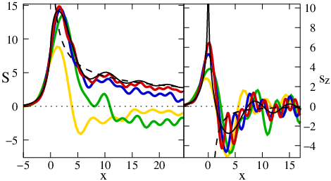
Numerical calculations presented in Fig. 4 illustrate the emergence of the logarithmic peak when the slope of the boundary potential decreases, Eq. (9).
In Summary, we have predicted that the nonequilibrium spin-Hall spin accumulation near a smooth boundary of 2DEG ballistic conductor with spin-orbit interaction develops a narrow peak at the edge, with the width and height given by Eq. (9). It is followed by a slow non-monotonic decay, see Fig. 2. This smooth tail of spin density persists to much larger distances, . The amount of spin accumulated in the peak (found as a maximum of the function ) equals , where in the last inequality we utilize the fact that . We thus conclude that the spin accumulated at the edge described by a semiclassical boundary potential is inversely proportional to the strength of spin-orbit interaction and becomes progressively larger for smoother slopes. This prediction can be used for experimental observation of spin-Hall effect in realistic two-dimensional electron systems.
This work was supported by the SFB TR 12 and DOE Grant No. DE-FG02-06ER46313.
References
- [1] Present Address: Department of Physics, University of Texas, Austin, TX 78712, USA.
- [2] M.I. Dyakonov, V.I. Perel, Phys. Lett. A 35, 459 (1971).
- [3] Y.K. Kato, et al., Science 306, 1910 (2004);
- [4] V. Sih, et al., Nature Physics 1, 31 (2005).
- [5] S.O. Valenzuela and M. Tinkham, Nature 442, 176 (2006).
- [6] J. Wunderlich, et al., Phys. Rev. Lett. 94, 047204 (2005).
- [7] J.E. Hirsch, Phys. Rev. Lett. 83, 1834 (1999).
- [8] Shufeng Zhang, Phys. Rev. Lett. 85, 393 (2000).
- [9] H.A. Engel, B.I. Halperin, and E.I. Rashba, Phys. Rev. Lett. 95, 166605 (2005).
- [10] W.-K. Tse, S. Das Sarma, Phys. Rev. Lett. 96, 056601 (2006).
- [11] S. Murakami, N. Nagaosa, and S.-C. Zhang, Science 301, 1348 (2003).
- [12] J. Sinova, et al., Phys. Rev. Lett. 92, 126603 (2004).
- [13] J.I. Inoue, G.E.W. Bauer, and L.W. Molenkamp, Phys. Rev. B 70, 41303(R) (2004).
- [14] E.G. Mishchenko, A.V. Shytov, and B.I. Halperin, Phys. Rev. Lett. 93, 226602 (2004).
- [15] A. Khaetskii, Phys. Rev. Lett. 96, 056602 (2006).
- [16] R. Raimondi and P. Schwab, Phys. Rev. B 71, 33311 (2005).
- [17] O.V. Dimitrova, Phys. Rev. B 71, 245327 (2005).
- [18] This exact cancellation does not occur in 3D- or 2D hole-systems that feature non-linear spin-orbit couplings.
- [19] S. Murakami, Adv. in Solid State Phys. 45, 197 (2005).
- [20] H.A. Engel, E.I. Rashba, and B.I. Halperin, Theory of Spin Hall Effects in Semiconductors, in Handbook of Magnetism and Advanced Magnetic Materials, H. Eds. Kronmüller and S. Parkin (John Wiley & Sons, 2007).
- [21] Non-local detection of spin Hall currents in multiterminal devices has recently been reported in K.C. Weng, et al., arXiv:0804.0096; C. Bruene, et al., arXiv:0812.3768.
- [22] K. Nomura, et al., Phys. Rev. B 72, 245330 (2005).
- [23] B.K. Nikolic, et al., Phys. Rev. B 72, 075361 (2005); B.K. Nikolic, et al., Phys. Rev. Lett. 95, 046601 (2005).
- [24] E.M. Hankiewicz, et al., Phys. Rev. B 70, 241301(R) (2004).
- [25] G. Usaj and C.A. Balseiro, Europhys. Lett. 72, 631 (2005); A. Reynoso, G. Usaj and C.A. Balseiro, Phys. Rev. B 73, 115342 (2006).
- [26] T.D. Stanescu and V. Galitski, Phys. Rev. B 74, 205331 (2006).
- [27] V.A. Zyuzin, P.G. Silvestrov, and E.G. Mishchenko, Phys. Rev. Lett. 99, 106601 (2007).
- [28] Yu.A. Bychkov and E.I. Rashba, J. Phys. C 17 6039 (1984); F.T. Vas’ko, JETP Lett. 30, 540 (1979).
- [29] L.D. Landau, and E.M. Lifshitz, Quantum Mechanics (Pergamon Press, Oxford, 1976).
- [30] P.G. Silvestrov and E.G. Mishchenko, Phys. Rev. B 74, 165301 (2006).