ANL-HEP-08-76 EFI-08-29 FERMILAB-PUB-08-561-T MCTP-08-47 Minimal Flavor Violation and the Scale of Supersymmetry Breaking
Abstract
In this paper we explore the constraints from B-physics observables in SUSY models of Minimal Flavor Violation, in the large regime, for both low and high scale supersymmetry breaking scenarios. We find that the rare B-decays and can be quite sensitive to the scale at which supersymmetry breaking is communicated to the visible sector. In the case of high scale supersymmetry breaking, we show that the additional gluino contribution to the and rare decay rates can be significant for large , and . The constraints on are relatively insensitive to the precise scale of . We also consider the additional constraints from the present direct Higgs searches at the Tevatron in the inclusive channel, and the latest CDMS direct dark matter detection experiments. We find that altogether the constraints from B-physics, Higgs physics and direct dark matter searches can be extremely powerful in probing regions of SUSY parameter space for low and large , leading to a preference for models with a lightest CP-even Higgs mass close to the current experimental limit. We find interesting regions of parameter space that satisfy all constraints and can be probed by Higgs searches at the Tevatron and the LHC and by direct dark matter searches in the near future.
1 Introduction
The next few years promise to be extremely exciting for High Energy Physics because of new results coming from the Tevatron collider, the expected start of the LHC and a number of dark matter detection experiments. It is hoped that all this experimental data will shed some light on the mechanism of electroweak symmetry breaking and possibly on the origin of dark matter in the universe.
Theoretically, one of the more promising scenarios that can explain both questions is that of low energy supersymmetry. In particular, the minimal supersymmetric extension of the Standard Model (MSSM) with R-parity can both stabilize the electroweak scale and provide a cold dark matter candidate (i.e. the lightest neutralino) with a relic abundance that is in good agreement with the WMAP value [1]
| (1) |
However, like most extensions of the Standard Model, the MSSM is highly constrained by flavor changing effects, in particular through B-physics observables. These constraints can be naturally satisfied if the SUSY breaking terms are approximately flavor diagonal at the scale , at which supersymmetry breaking is communicated to the visible sector, and all flavor changing effects are loop induced and proportional to the elements of the CKM matrix of the Standard Model. Such supersymmetric extensions of the Standard Model are generically called Minimal Flavor Violating (MFV) and have been extensively studied in Refs. [2]–[16]. In particular, in Ref. [15] the impact of maximal CP-violation and minimal flavor violating MSSM is considered. At large , the ratio of the two Higgs vacuum expectation values in the MSSM, flavor changing neutral currents (FCNCs) are induced by the Higgs sector through loop effects that can lead to significant deviations in B-physics observables from their Standard Model predictions. The B-factories, Belle and Babar, and the Tevatron have measured many of these observables and these data put strong constraints on the allowed MSSM parameter space.
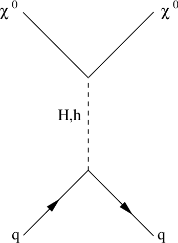
Simultaneously, experiments are also trying to discover the footprint of supersymmetry through dark matter searches of a stable neutralino. These searches for dark matter have also begun to put significant constraints on supersymmetric models by providing limits on the spin-independent scattering cross-sections of the lightest neutralino with nuclei. In the MSSM, the couplings of the down type quarks to the non-standard Higgs bosons are enhanced. Therefore the t-channel Higgs boson contribution to this cross-section can be sufficiently enhanced for small enough values of the non-standard CP-even Higgs boson mass and large . In addition the spin-independent cross-section also depends on the size of the Higgsino component of the lightest neutralino which is governed by the Higgsino mass parameter . The impact of direct dark matter searches on Higgs physics has been analysed in Refs. [17, 18, 19].
In this article we study the effect of varying the scale , at which supersymmetry breaking is communicated to the visible sector, on B-physics observables in the context of Minimal Flavor Violation. We concentrate on two scenarios of supersymmetry breaking: low-scale, , and high-scale, , SUSY breaking, where and represent the scale of the supersymmetric particle masses and the Grand Unification scale, respectively. In the case of low scale supersymmetry breaking the flavor changing effects are governed by loop induced Higgs mediated currents. In the case of high scale SUSY breaking, the soft squark mass terms are logarithmically sensitive to the scale , due to their RG evolution. In particular for large supersymmetry breaking scales the soft squark mass parameters pick up off-diagonal contributions proportional to the CKM matrix elements. Hence the squark and quark mass matrices cannot be diagonalized simultaneously. This mismatch between the quark and squark mass bases induces flavor violating quark-squark-gluino couplings that are proportional to the CKM matrix elements, which lead to important gluino contributions to both the and rare decays, in addition to those already present when .
In order to analyze the size of the possible gluino effects, we shall study scenarios that parametrize the possible flavor violation effects in models of Minimal Flavor Violation with a small messenger scale , of the order of the weak scale, and with a large scale , of the order of the GUT scale, respectively. In the first scenario, we shall assume no flavor violating quark-squark-gluino couplings. In the second scenario, we shall assume a left-handed squark mass matrix that is diagonalized together with the up Yukawa coupling matrix, as would be the case if the down Yukawa effects in the RG evolution of the soft masses were neglected compared to those of the up Yukawas. The effect of the non-diagonal left-handed down type quark-squark-gluino vertices on the rare decay within this approximation has been previously computed in Ref. [7]. In this article we derive an analytic formula for the gluino contribution to the rare decay for large values of , within the same approximation. The validity of this approximation will be discussed in section 2.1.2.
In addition we also study the interplay between the B-physics constraints from the , and the rare decays and the recent direct dark matter detection limits from CDMS [20].Let us stress here that low energy SUSY breaking scenarios lead to a light gravitino and therefore the CDMS constraints would not apply. We find that combining the limits from B-physics observables, dark matter detection experiments at CDMS and inclusive searches at the Tevatron [24] yields interesting constraints on the and plane, where is the CP-odd Higgs mass and is the stop left-right mixing parameter. We find regions of parameter space that satisfy all these constraints and can be probed by Higgs searches at the Tevatron and by direct dark matter searches in the near future.
The paper is organized as follows, in Section 2 we consider the effect of the scale on B-physics observables in minimal flavor violating MSSM. In particular we present the additional gluino contributions to the and rare decays. The complete calculation of the gluino contribution to the decay can be found in Appendix A. We also give a brief theoretical overview of the relevant direct dark matter detection cross-section. In Section 3 we consider different parametric scenarios that can satisfy the B-physics experimental constraints, the limits coming from inclusive searches at the Tevatron and the direct dark matter detection limits from CDMS. In particular we explore the dependence of our results on the scale at which supersymmetry breaking is communicated to the visible sector. In Section 4 we present our conclusions.
2 Basic Theoretical Setup
2.1 B-physics Constraints and messenger mass scale
The FCNCs induced by loops of squarks depend on the flavor structure of the soft squark mass parameters which, in MFV, is closely tied to the scale at which supersymmetry breaking is communicated to the visible sector 11 1 Unlike Ref. [26], we are considering the case where effects from the hidden sector are small. Assuming the squark masses are flavor independent at high scales, the only one-loop corrections that violate flavor are due to RG effects governed by the up and down Yukawa matrices, since the gauge interactions are flavor blind. The corrections to the left-handed soft SUSY breaking mass parameter at one-loop are given by [27]
| (2) | |||||
where denotes the left-handed squark mass matrix, is the right-handed up (down) squark mass matrix, and are the Higgs soft supersymmetry breaking and squark-Higgs trilinear mass parameters, respectively, at the messenger scale , at which supersymmetry breaking is transmitted to the observable sector, and is the characteristic low energy squark mass scale. Similarly, the right-handed up and down squark mass matrices, receive one-loop Yukawa-induced corrections proportional to
| (3) |
and
| (4) |
respectively. Hence the corrections to the right-handed soft mass parameters are diagonal in the quark basis, but the left-handed soft mass parameters of the down squarks pick up off-diagonal contributions proportional to the CKM matrix elements. The size of these corrections depends on the scale at which SUSY breaking is communicated to the visible sector. If is of the order of then these corrections are small and if then these corrections can be substantial. In this section we consider the effect of these two scenarios on three B-physics processes , and .
2.1.1
In the case the squark mass matrices are approximately block diagonal which leads to all the neutral Higgs induced FCNCs being proportional to the chargino-stop loop factor , with [5]
| (5) |
where
| (6) |
No flavor changing effects are produced by contributions from the gluino down squark loop as they are purely flavor diagonal
| (7) |
where and are the Ith down squark mass eigenstates. The effective flavor changing strange-bottom-neutral-Higgs coupling is [5, 8, 16]
| (8) |
where
| (9) | |||||
| (10) | |||||
| (11) |
in the basis ().
At large values of the dominant supersymmetric contributions to rare decay are mediated by neutral Higgs boson exchange that leads to [5, 25]
| (12) |
Therefore, in this scenario, the magnitude of this observable is suppressed when is small compared to .
As the gluino-quark-squark vertex is flavor diagonal for the dominant SUSY contributions to the rare decay come from the charged-Higgs boson and the chargino-stop loops. In particular the Wilson coefficients due to the charged Higgs contribution are proportional to the factor [28, 29]
| (13) |
while the Wilson coefficient due to the chargino-stop loop has the form [28, 29]
| (14) |
where is the loop integral appearing at one loop. Eq. (13) includes the resummed contributions and the prescription used in Refs. [28, 29],
| (15) | |||
| (16) | |||
| (17) |
where, is the correction to the charged-Higgs-top-strange vertex due to the gluino-stop loop and is the stop mixing angle.
The dominant supersymmetric contribution to the rare decay is due to the charged Higgs which interferes with the Standard Model contribution and we can define the ratio [30]
| (18) |
so as to quantify deviations from the Standard Model in this process.
In addition, Ref. [31] has shown the importance of Kaon semi-leptonic decays in constraining the charged Higgs contribution to the rare decay. In particular they consider the quantity
| (19) |
where the subscript refers to semileptonic decays with final states and refers to beta decay. For the Standard Model, while when a charged Higgs is included we have
| (20) |
The charged Higgs constribution in Eq. (20) and Eq. (18) are the same and limits on can be a strong constraint on the scenario in which SUSY contributions to the dominate those of the Standard Model. Assuming that is the largest allowed negative deviation of from one and is the smallest allowed value of , we see that for the charged Higgs to dominate over the SM contributions in Eq. (18) the deviations must satisfy the constraint
| (21) |
Hence, a two sigma experimental bound on would strongly disfavor scenarios in which the charged Higgs contribution to the decay is larger than that of the Standard Model.
2.1.2
When , corrections to the soft masses due to RG evolution are log enhanced. Therefore, if we neglect the term in Eq. (2), the left-handed down squark mass matrix is diagonalized by the matrix which diagonalizes the up-quark mass matrix, rather than the down quark diagonalizing matrix . Neglecting the corrections due to the bottom Yukawa over-estimates the splitting between the third and first two generations of down squark masses and is not valid when or when is large. For and of the order of , with positive, one obtains and therefore the bottom Yukawa,
| (22) |
becomes equal to for values of . The parametrization used in this article increases in accuracy as takes smaller values, and also for larger values of , for which the above corrections to the bottom Yukawa coupling become significant, therefore reducing the value of . In this article, we shall assume that . In addition, as we shall discuss below, present experimental constraints lead to a preference for moderate or large values of at sizable values of and small values of . Therefore, we expect our parametrization to lead to a good approximation of the gluino induced effects in the scenarios discussed in this article. Furthermore using this approximation we were able to reproduce the the numerical B-physics limits obtained by Ref. [11], where the full renormalization group evolution of the mass parameters was performed.
In the approximation, in which the left-handed down squarks are diagonalized by , flavor violating vertices proportional to the CKM matrix in the gluino-down squark-down quark interaction vertex are induced,
| (23) |
and the soft SUSY breaking down-squark mass Lagrangian takes the form
| (24) |
where . Due to the gluino-quark-squark couplings being non-diagonal there are additional contributions to both the loop induced and rare decays, but no large additional contributions to the process.
For , the effective flavor changing strange-bottom-neutral-Higgs coupling is [7]
| (25) |
where we have assumed that the first two generations of left-handed down squark masses are , the uniform right-handed down squark soft mass parameters are and
| (26) |
In the limit of the left-handed sbottom mass being equal to that of the first two generations, Eq. (25) reduces to Eq. (8). In the scenario, the dominant SUSY contribution to rare decay, at large , is found by substituting the form of in Eq. (25) into Eq. (12). The present experimental limit on disfavors very large positive contributions due to new physics effects. In high scale SUSY breaking, the new physics contributions to the rare decay process are suppressed if the splitting in the left-handed down-type squarks soft mass parameters is such that is rendered small. As this suppression may be significant whenever , where the value of , that allows such a cancellation, increases with the splitting of down squark masses and therefore with the messenger mass scale .
Futhermore, flavor violation in the gluino sector also induces relevant gluino contributions to the rare decay [34, 35]. In Appendix A we find that, within the approximation of Eq. (23) and Eq. (24), the Wilson coefficients due to these gluino contributions are
| (27) | |||||
where , is the left-handed third generation down squark mass, is the sbottom mass, , , and the functions are defined in Eq. (97) 22 2 A calculation of the gluino effects valid in the more general case has been recently performed in Ref. [36]. As expected this contribution to rare decay also disappears in the limit of uniform left-handed down squark soft mass parameters . For non-zero mass splittings, these contributions are important at large and in the absence of CP violation are proportional to the sign of . Therefore if is positive the gluino contribution adds to that of the charged Higgs while when it is negative it subtracts from the charged Higgs contribution.

In Fig. 1 we plot the relative gluino contribution to the decay branching ratio , defined as
| (28) |
for two different sets of SUSY parameters. The solid curve corresponds to the value of for superymmetric parameters GeV and , while for the dashed curve we consider TeV. The splitting between the third and first two generations of squark masses is 20% and GeV. We see that, in general, the gluinos lead to a moderate modification of . For instance, in the example shown in Fig. 1, the gluino effects lead to at most a 10-15% contribution to . In addition, since is positive for these points, the gluino contribution to the is also positive.
2.2 Direct dark matter detection through Higgs exchange
The spin-independent elastic scattering cross-section for a neutralino scattering off a heavy nucleus is:
| (29) |
where , is the mass of the nucleus, is the neutralino mass,
| (30) | |||||
| (31) | |||||
| (32) |
and the quark form factors are and [17]. In Eq. (31) and Eq. (32) is the neutralino rotation matrix, is the CP-even Higgs rotation angle and () is the lighter (heavier) CP-even Higgs mass. Also in the above expression we define
| (33) |
for the first two generations of quarks and
| (34) |
for the bottom quark. In Eq. (32), we are ignoring the contribution from s-channel squark exchange, which becomes subdominant for heavy squark masses. In the limit of large is enhanced compared to . Moreover, for large , , and GeV ( GeV), one obtains , () and (). Hence we find that the dominant contribution is
| (35) | |||||
| (36) |
where we have neglected, in the first line, the splitting between the first two generations of squarks and, in the second line, the differences between the proton and the neutron mass and we used the fact that the neutron and proton factors are relatively similar. Assuming that the mass of the neutralino is much larger than that of the nucleus we have and
| (37) | |||||
| (38) |
where is the neutralino nucleon spin-independent cross-section. From Eq. (38) the spin-independent cross-section scales as and therefore direct dark matter detection experiments like CDMS can put strong constraints on regions of small and large .
3 Numerical limits and constraints
3.1 Experimental constraints on B-physics observables.
Due to the extra supersymmetric contributions to these rare decays we find that experimental data put strong constraints on these models. In particular, the world experimental average of the branching ratio of the rare decay is [38]
| (39) |
which agrees well with the Standard Model prediction [39]
| (40) |
Using the experimental and SM ranges for the rare decay we find the allowed range is
| (41) |
For the rare decay the Belle experimental collaboration measures a branching ratio of [40]
| (42) |
while the Babar collaboration finds the preliminary value [41]
| (43) |
The average of these two experiments is then [42]
| (44) |
Using MeV from LQCD [42] and the average value of from HFAG [43], the Standard Model prediction is
| (45) |
Assuming at most a 2 deviation from new physics, we find the allowed range
| (46) |
For the constraint in Eq. (20), Ref. [31] finds that
| (47) |
when they use the value of from Ref. [32]. However if we use the average value of from Ref. [33]
| (48) |
In this paper we will use this more conservative limit on the rather than the one in Eq. (47). From Eq. (21) it is clear that the more restrictive bound in Eq. (47) strongly disfavors the regions of low and large that are allowed by the constraint in Eq. (46), where the charged Higgs contribution to the process dominates that of the Standard Model.
The rare decay has yet to be experimentally observed. The present experimental exclusion limit at 95% C.L. from CDF [44] is
| (49) |
which can put strong restrictions on possible flavor changing neutral currents in the MSSM at large . Additionally the projected exclusion limit, at 95% C.L., on this process for 4 fb-1 at the Tevatron is [45]
| (50) |
For the LHC, the projected ATLAS bound at 10 fb-1 is [46]
| (51) |
In addition, LHCb has the potential to claim a evidence (discovery) of a standard model signature with as little as fb-1(fb-1) of data [47].
3.2 Direct dark matter detection constraints.
As discussed in Section 2.2 the spin-independent scattering cross-section for a neutralino off a heavy nucleus scales as and therefore puts strong constraints on the SUSY parameter space. At present the CDMS [20] and XENON [48] collaborations have put a limit on the spin-independent neutralino-nucleon cross-section that is of the order of pb [21]. We will use the CDMS limits throughout this paper because we only consider neutralino masses greater than GeV and the current limits from the CDMS experiment are slightly stronger than those from XENON [21] for these range of masses. By the end of 2009, the sensitivity of the XENON100 experiment will improve by an order of magnitude [22], while the sensitivity of the SuperCDMS experiment will improve by factor of 5 [23]. Therefore in the near future, these direct dark matter detection experiments will be able to probe regions of SUSY parameter space that will also be probed by the Tevatron in non-standard Higgs searches.
3.3 Parametric scenarios
Due to the dependence on the messenger scale we consider different scenarios to illustrate the interplay between B-physics, Higgs physics and dark matter searches within the framework of the MSSM with large . In this section we will assume the gaugino unification relation and that all the gauginos have equal phases. We shall consider four parameters: the CP-odd Higgs mass , the ratio of the two Higgs vacuum expectation values , the Higgsino mass parameter and , where is the stop-Higgs trilinear coupling. In order to consider the direct dark matter detection constraints, we will also assume that the total relic density agrees with that found by WMAP, independently of the squark, neutralino and Higgs spectrum. This may require an appropriate slepton spectrum or a departure from the standard thermal dark matter predictions [49]. In addition we considered the non-standard Higgs boson search limits in Ref. [24, 50, 51] and used the CPsuperH [52] program to project these constraints onto the plane. Even though the Tevatron will be collecting about fb-1 of data, the projected fb-1 CDF limit provides a conservative estimate of the final reach of the Tevatron in the channel because a realistic treatment of the detector and efficiencies may lead to somewhat weaker constraints than those shown in Ref. [50]. The future LHC constraints on the channel, from Ref. [51], correspond to the projected limits at ATLAS for fb-1 of data.
The good agreement between the Standard Model prediction and the experimental measurement of the branching ratio of implies that either there is some cancellation between the dominant new physics leading order Wilson coefficients in Eq. (13) and Eq. (14) or each of them are individually small. If is sizable and the sign of is negative then a cancellation between the chargino-stop and charged Higgs Wilson coefficients is possible for large enough values of . For negligible values of the chargino-stop contribution is suppressed, which requires the charged Higgs amplitude to be small. This suppression of the charged Higgs Wilson coefficient can be achieved by making the bottom-top-charged-Higgs vertex small through a cancellation between the tree-level coupling and the one loop enhanced correction in Eq. (13). In addition to the leading order contribution we have also included the next-to-leading order contributions due to the charged Higgs as discussed in Ref. [37]. Additionally there is also a possible gluino contribution that can be significant if the squark masses are splitted. The gluino contribution, for the scenario in which , is relevant for large , and and depending on the sign of this contribution interferes constructively or destructively with the other two contributions.
Similarly to the rare decay, the rare decay is sensitive to the scale at which supersymmetry breaking is communicated to the visible sector. Depending on the scale the structure of the couplings in Eq. (8) and Eq. (25) is different. If , this coupling is suppressed if or equivalently is small compared to or . However if is large compared to then splittings in the squark masses, due to RG evolution, can induce a suppression of this coupling, due to a cancellation between the stop-chargino and sbottom gluino loops.

The bound in Eq. (46) imposes a complementary constraint to that of . The lower bound of implies that there cannot be complete destructive interference between the SUSY and Standard Model contributions. Therefore there are two disconnected allowed regions in the plane: one where the charged Higgs induced amplitude dominates the Standard Model contribution and the other where the opposite happens.
In these kind of scenarios, Eq. (38) suggests that the spin-independent dark matter scattering cross-section is quite sensitive to the amount of the Higgsino component in the lightest neutralino. At low values of there is a large Higgsino component to the lightest neutralino and hence a larger scattering cross-section through t-channel CP-even Higgs bosons. For large values of , instead, the Higgsino component is much smaller, and so the coupling of the neutralino to the Higgs is suppressed leading to a smaller cross-section. In addition, the sensitivity of direct dark matter detection experiments, like CDMS, to the spin independent cross-section decrease with increasing LSP mass for GeV. Observe, however that the CDMS constraint assumes the neutralino to be the dark matter candidate while in low SUSY breaking scenarios the LSP is naturally the gravitino, and therefore these constraints should not apply.
Throughout this section we set the uniform left-handed soft squark mass parameter for the first two generations to TeV, the third generation soft squark mass parameters are TeV and the uniform right-handed down squark soft mass parameter is TeV. This form of the left handed down squark soft masses has been chosen so as to mirror a 20% splitting in the soft masses due to their renormalization group evolution in scenario, as is naturally the case whenever the gaugino masses are of the same order as the scalar masses at the scale . We have chosen a value of the third generation squark

masses slightly larger than 1 TeV, in order to satisfy the lightest CP-even Higgs mass constraints for all the scenarios under study. For the scenario we shall assume a degenerate squark spectrum with soft masses of 1.2 TeV. In this way, we can compare the results with those in the case for which the third generation masses, most relevant in the calculation of the B-physics observables, have also values of 1.2 TeV.
In Fig. 3 and Fig. 4 we present the effects of the B physics constraints and the CDMS direct dark matter detection experiment limit on the plane for , and respectively. These two sets of values correspond to regions of parameter space which are close to being probed at the Tevatron in inclusive searches [24]. The green (grey) hatched region is the one allowed by the , and constraints for , while the yellow (light grey) region is allowed by the same constraints for scenario. The constraint does not depend on the parameter and therefore the constraint in Eq. (46) selects a horizontal band in the plane. The regions below the solid and dashed red (dark grey) lines is excluded by CDMS, for GeV and GeV, respectively.
In Fig. 3, for GeV and , The extra gluino contributions to the and, most relevantly, the rare decay rates, leads to a modification of the preferred values of . While the B-physics constraints lead to a preference for small values of in the scenario, moderate values of GeV are preferred in the case. Assuming that the LSP is the neutralino, which is natural in the scenario, the recent CDMS limits [20] are quite strong and exclude regions below

GeV. Indeed, for these values of and we observe that large to moderate values of are preferred for both SUSY breaking scenarios.
Fig. 4 shows the situation for GeV and . Similar to Fig. 3 small values of are preferred in the scenario while moderate values of GeV are preferred in the scenario. For these values of and , the CDMS experimental bound is less stringent than in Fig. 3, restricting values below GeV in the scenario. Similar to Fig. 3, the constraint is the main discriminant between the and scenarios.
From Figs. 3 and Fig. 4 we can observe some generic features. Independent of the SUSY breaking scale, for these regions of parameter space, that can be probed at the Tevatron, one obtains that . These low values of the stop-mixing parameter imply an upper bound on the lightest CP-even Higgs boson mass, GeV and therefore could be within the reach of the Tevatron collider. As we had previously emphasized the regions close to and are yet to be probed at the Tevatron in searches at fb-1. Using Figs. 3 and 4 we see that the region of parameter space around and satisfies all the constraints in the scenario. In addition, from Fig. 4, we also find that the region of parameter space close to satisfies all constraints for . As the constraints from B-physics, Higgs physics and direct dark matter searches get stronger this kind of analysis could help us identify regions of parameter space that would still be compatible with all experimental limits.
In Fig. 5 we consider the GeV and GeV parametric scenario. The region above the solid and dashed red (dark grey) lines has been probed by CDMS in direct dark matter detection experiments, for a Wino mass parameter GeV and GeV respectively. The blue-green (medium grey) region is excluded by CDF and D0 in non-standard Higgs boson searches in the channel at 1.8 fb-1. The green (grey) hatched region is allowed by the experimental constraints on the , and rare B decays for while the yellow (light grey) region corresponds to the same constraints for the scenario. The region above the black solid (dashed) lines

will be probed in the channel at the Tevatron (LHC) with a luminosity of fb-1 ( fb-1). In this parametric scenario, with and and the different contributions tend to cancel against each other. The chargino-stop approximately cancels the charged Higgs contribution in the scenario, while in the scenario the chargino contribution tends to cancel both the charged Higgs and the gluino contributions. There are two regions allowed by constraint. The allowed region at low and large is where the supersymmetric contribution dominates, while in the large and low to moderate region the Standard Model contribution dominates. The constraint is quite strong for the scenario due to a non-zero , excluding most of the region where the charged Higgs contribution to becomes dominant, while for the a cancellation is induced in the flavor violating effects due to the splitting of the left-handed down squark soft mass parameters.
In Fig. 5 we see that somewhat smaller values of are allowed in the case than in the case. This effect may be explained by the gluino contributions to : For positive values of a larger chargino-stop contribution is required to get agreement with the experimental values, which may be obtained for larger values of . The constraint in Eq. (48) becomes too weak to give any significant constraint in Fig. 5 and in the other scenarios we consider in this paper. Let us stress again, if we had considered the more restrictive bound on in Eq. (47) the region of low and large allowed by the other flavor constraints would be strongly disfavored.
As Fig. 3 suggested the region of small and 35–45 is allowed by all the B physics constraints and has yet to be probed by the Tevatron in inclusive searches. The allowed region is larger for than for . For , this region is however also constrained by direct dark matter detection experiments like CDMS as can also be seen in Fig. 5. In addition, there is also a region around that is allowed in the scenario, which has yet to be probed in direct dark matter detection experiments and non-standard Higgs searches. However the XENON100 and SuperCDMS experiments should be able to probe this region of parameter space in the near future due to their improved sensistivity.
In Fig. 6 we consider a scenario where TeV and . The chargino-stop contribution to the rate is small in this scenario, because , while the charged Higgs contribution tends to be suppressed because of a cancellation between the 1-loop and 2-loop contributions in Eq. (13). The constraint for the scenario is strong because there is no cancellation that occurs in Eq. (25), while it is weak in the scenario because . In addition there are two regions around and that are allowed by all these constraints in the scenario but disallowed in the scenario. As in the previous case, a significant region of parameters consistent with all experimental appears at low values of and large values of but in this case is compatible with and hence no CDMS restrictions apply. In addition both Fig. 5 and Fig. 6 also show that the Tevatron collider will be able to probe all these allowed regions in non-standard Higgs boson searches with a luminosity of fb-1. Futhermore, in both these scenarios, the LHC will be able to probe more of the allowed regions of large and low , in the channel with fb-1 of luminosity.
4 Conclusion
In this article we have studied the effect of varying the messenger scale on B physics observables within Minimal Flavor Violating supersymmetric models. In particular we found that the and rare decays are sensitive to the scale at which supersymmetry breaking is communicated to the visible sector. Considering the effects of the RG evolution which amounts to an alignment of the left-handed squark masses with the up Yukawa couplings, with uniform right-handed down squark soft masses and also uniform left-handed down squark masses of the first two generations, we have derived an analytic expression for the gluino contribution to the rare decay. We find that the gluino contribution is proportional to the splitting between the third generation left-handed down squark mass and that of the first two generations. The relative sign of the gluino contribution to that of charged Higgs depends on the sign of . Hence in the case of the messenger scale , when the splitting in the left-handed squark masses is non-zero, this contribution can be significant. In addition we also show the dependence of the dominant SUSY penguin contributions to the rare decay on the scale .
We have also studied the interplay between the B-physics constraints, dark matter direct detection experiments and non-standard Higgs boson searches at the Tevatron. For large soft squark masses, the spin-independent neutralino nucleon cross-section is proportional to and hence direct detection experiments put strong constraints on regions of low ( GeV) and large . In particular, we have projected the CDMS direct dark matter detection experimental constraint on the plane, for different values of and . Independently of the messenger scale , the B physics, Higgs physics and Dark Matter experimental constraints suggest that low values of and large to moderate values of are preferred. Such low values of generally suggests an approximate upper bound on the lightest Higgs mass GeV, which may be within the reach of the Tevatron collider.
In addition, we have presented parametric scenarios that satisfy all the B physics experimental constraints considered in this article, within the scenarios of low scale () and high scale () supersymmetry breaking, and can be probed by the Tevatron collider and the LHC in the near future. In particular for we find a region around GeV and , and moderate values of and , which is within the fb-1 reach of the Tevatron collider in non-standard Higgs searches. For , instead, smaller values of and moderate or large values of are preferred, in order to obtain acceptable values of and . Moreover, we showed that for , there are large regions of parameter space for low and large that remain to be probed by non-standard Higgs searches at the Tevatron collider. Apart from a region at similar values of and as the ones arising in the scenario, we found an additional region, for smaller values of GeV and . This region only appears in scenarios with low energy supersymmetry breaking, since it is constrained by direct dark matter searches in the scenario.
Our analysis suggests that, in Minimal Flavor Violating MSSM, future Higgs searches at the Tevatron and direct dark matter detection experiments at CDMS and XENON will reveal useful information about SUSY parameters and the scale of supersymmetry breaking. For instance, the detection of a light non-standard Higgs boson at the Tevatron and dark matter at the XENON and CDMS experiments, by the end of 2009, would suggest a scenario, from which we can infer moderate values of , large to moderate values of and a Standard Model Higgs boson mass GeV. On the other hand, detection of a light non-standard Higgs boson and non-detection of dark matter may suggest a lower SUSY breaking messenger scale, small values of , large values of and a Standard Model Higgs boson mass close to that of the LEP experimental limit.
Acknowledgments
Work at ANL is supported in part by the US DOE, Div. of HEP, Contract DE-AC02-06CH11357. Fermilab is operated by Fermi Research Alliance, LLC under Contract No. DE-AC02-07CH11359 with the United States Department of Energy. A.M. was also supported by MCTP and DOE under grant DE-FG02-95ER40899. We would like to thank the Aspen Center for Physics and the KITPC, China, where part of this work has been done.
Appendix A Gluino contribution to
In the initial gauge basis the gluon-quark-squark interaction Lagrangian has the form
| (52) |
Rotating the quarks into the mass basis by the matrices
| (53) | |||
| (54) |
and the down squarks by the matrices
| (55) |
so as to diagonalize the down squark soft masses. Hence the gluon-quark-squark interaction Lagrangian becomes
| (56) | |||||
| (57) |
However this rotation induces off-diagonal terms to the left-right and right-left blocks of the down-squarks, so that,
| (58) |
where we have neglected terms proportional to the down and strange Yukawa’s and . Hence all three of the left-handed states mix with . As we explicitly diagonalize the sector so that
| (59) | |||||
| (60) |
where
| (61) | |||||
| (62) | |||||
| (63) | |||||
| (64) | |||||
| (65) | |||||
| (66) |
which leads to
| (67) | |||||
| (68) | |||||
To leading order in the CKM matrix elements we can further diagonalize the left-handed states so that
| (69) | |||||
| (70) | |||||
| (71) | |||||
| (72) | |||||
| (73) | |||||
| (74) |
Hence
| (75) | |||||
where we have neglected higher orders in the CKM matrix. Therefore the vertex factors are
Now rewriting the following identity in Eq. (64)
| (90) |
we have
| (91) | |||||
| (92) | |||||
| (93) | |||||
| (94) | |||||
| (95) |
Hence using the amplitudes defined in Ref. [2] we find the Wilson coefficients
| (96) | |||||
where
| (97) | |||||
References
- [1] D. N. Spergel et al. [WMAP Collaboration], Astrophys. J. Suppl. 170, 377 (2007) [arXiv:astro-ph/0603449].
- [2] S. Bertolini, F. Borzumati, A. Masiero and G. Ridolfi, Nucl. Phys. B 353, 591 (1991).
- [3] G. Isidori and A. Retico, JHEP 0111, 001 (2001) [arXiv:hep-ph/0110121].
- [4] A. J. Buras, P. H. Chankowski, J. Rosiek and L. Slawianowska, Phys. Lett. B 546, 96 (2002) [arXiv:hep-ph/0207241].
- [5] A. J. Buras, P. H. Chankowski, J. Rosiek and L. Slawianowska, Nucl. Phys. B 659, 3 (2003) [arXiv:hep-ph/0210145].
- [6] K. S. Babu and C. F. Kolda, Phys. Rev. Lett. 84, 228 (2000) [arXiv:hep-ph/9909476].
- [7] A. Dedes and A. Pilaftsis, Phys. Rev. D 67, 015012 (2003) [arXiv:hep-ph/0209306].
- [8] D. A. Demir, Phys. Lett. B 571, 193 (2003) [arXiv:hep-ph/0303249].
- [9] E. Lunghi, W. Porod and O. Vives, Phys. Rev. D 74, 075003 (2006) [arXiv:hep-ph/0605177].
- [10] J. R. Ellis, K. A. Olive, Y. Santoso and V. C. Spanos, JHEP 0605, 063 (2006) [arXiv:hep-ph/0603136].
- [11] J. R. Ellis, S. Heinemeyer, K. A. Olive and G. Weiglein, Phys. Lett. B 653, 292 (2007) [arXiv:0706.0977 [hep-ph]].
- [12] G. Isidori, F. Mescia, P. Paradisi and D. Temes, Phys. Rev. D 75, 115019 (2007) [arXiv:hep-ph/0703035].
- [13] G. Barenboim, P. Paradisi, O. Vives, E. Lunghi and W. Porod, JHEP 0804, 079 (2008) [arXiv:0712.3559 [hep-ph]].
- [14] P. Paradisi, M. Ratz, R. Schieren and C. Simonetto, Phys. Lett. B 668, 202 (2008) [arXiv:0805.3989 [hep-ph]].
- [15] J. R. Ellis, J. S. Lee and A. Pilaftsis, Phys. Rev. D 76, 115011 (2007) [arXiv:0708.2079 [hep-ph]].
- [16] J. Foster, K. i. Okumura and L. Roszkowski, JHEP 0508, 094 (2005) [arXiv:hep-ph/0506146].
- [17] G. B. Gelmini, P. Gondolo and E. Roulet, Nucl. Phys. B 351, 623 (1991). M. Srednicki and R. Watkins, Phys. Lett. B 225, 140 (1989). M. Drees and M.M. Nojiri, Phys. Rev. D 48, 3483 (1993) [arXiv:hep-ph/9307208]. J. R. Ellis, A. Ferstl and K. A. Olive, Phys. Lett. B 481, 304 (2000) [arXiv:hep-ph/0001005].
- [18] M. S. Carena, D. Hooper and P. Skands, Phys. Rev. Lett. 97, 051801 (2006) [arXiv:hep-ph/0603180].
- [19] M. S. Carena, D. Hooper and A. Vallinotto, Phys. Rev. D 75, 055010 (2007) [arXiv:hep-ph/0611065].
- [20] Z. Ahmed et al. [CDMS Collaboration], arXiv:0802.3530 [astro-ph].
- [21] http://dmtools.berkeley.edu/limitplots/
- [22] http://xenon.astro.columbia.edu/presentations/Aprile_IDM08.pdf
- [23] T. Bruch [CDMS Collaboration], AIP Conf. Proc. 957, 193 (2007).
- [24] http://www-cdf.fnal.gov/physics/new/hdg/results/htt_070928/ http://www-d0.fnal.gov/Run2Physics/WWW/results/prelim/HIGGS/H29/H29.pdf
- [25] M. S. Carena, A. Menon, R. Noriega-Papaqui, A. Szynkman and C. E. M. Wagner, Phys. Rev. D 74, 015009 (2006) [arXiv:hep-ph/0603106]. M. S. Carena, A. Menon and C. E. M. Wagner, Phys. Rev. D 76, 035004 (2007) [arXiv:0704.1143 [hep-ph]].
- [26] A. G. Cohen, T. S. Roy and M. Schmaltz, JHEP 0702, 027 (2007) [arXiv:hep-ph/0612100].
- [27] M. Dugan, B. Grinstein and L. J. Hall, Nucl. Phys. B 255, 413 (1985).
- [28] G. Degrassi, P. Gambino and G. F. Giudice, JHEP 0012, 009 (2000) [arXiv:hep-ph/0009337].
- [29] M. Carena, D. Garcia, U. Nierste and C. E. M. Wagner, Phys. Lett. B 499, 141 (2001) [arXiv:hep-ph/0010003].
- [30] W. S. Hou, Phys. Rev. D 48, 2342 (1993). A. G. Akeroyd and S. Recksiegel, J. Phys. G 29, 2311 (2003) [arXiv:hep-ph/0306037]. G. Isidori and P. Paradisi, Phys. Lett. B 639, 499 (2006) [arXiv:hep-ph/0605012].
- [31] M. Antonelli et al. [FlaviaNet Working Group on Kaon Decays], arXiv:0801.1817 [hep-ph]. D. Eriksson, F. Mahmoudi and O. St [] l, arXiv:0808.3551 [hep-ph].
- [32] E. Follana, C. T. H. Davies, G. P. Lepage and J. Shigemitsu, [HPQCD Collaboration and UKQCD Collaboration], Phys. Rev. Lett. 100, 062002 (2008) [arXiv:0706.1726 [hep-lat]].
- [33] http://conferences.jlab.org/lattice2008/talks/plenary/laurent_lellouch.pdf
- [34] B. Dudley and C. Kolda, arXiv:0805.4565 [hep-ph].
- [35] M. Wick and W. Altmannshofer, arXiv:0810.2874 [hep-ph].
- [36] G. Degrassi, P. Gambino and P. Slavich, Phys. Lett. B 635, 335 (2006) [arXiv:hep-ph/0601135].
- [37] M. Ciuchini, G. Degrassi, P. Gambino and G. F. Giudice, Nucl. Phys. B 527, 21 (1998) [arXiv:hep-ph/9710335].
- [38] E. Barberio et al. [Heavy Flavor Averaging Group (HFAG)], arXiv:hep-ex/0603003.
- [39] M. Misiak et al., Phys. Rev. Lett. 98, 022002 (2007) [arXiv:hep-ph/0609232].
- [40] K. Ikado et al., arXiv:hep-ex/0604018.
- [41]
B. Aubert et al. [BABAR Collaboration],
arXiv:hep-ex/0608019.;
New preliminary BABAR value obtained from http://www.slac.stanford.edu/xorg/hfag/rare/leppho07/
radll/OUTPUT/TABLES/radll.pdf - [42] M. Bona et al. [UTfit Collaboration], “The unitarity triangle fit in the standard model and hadronic parameters from lattice QCD: A reappraisal after the measurements of Delta(m(s)) and JHEP 0610, 081 (2006) [arXiv:hep-ph/0606167].; Update values obtained from http://www.utfit.org/
- [43] http://www.slac.stanford.edu/xorg/hfag/semi/LP07/home.shtml
- [44] R. Bernhard et al. [CDF Collaboration], arXiv:hep-ex/0508058.
- [45] See,for example, B. Heinemann presentation to the P5 Committee, Fermilab, September 2006, http://hep.ph.liv.ac.uk/ beate/homepage/p5-discovery.pdf
- [46]
Nikolai Nikitine, talk given
at ”FLAVOUR IN THE ERA OF THE LHC”
Opening plenary meeting: CERN, November 7-10 2005;
R. McPherson, talk given at the Aspen Winter Conference, Aspen, CO, February 12–18, 2006, http://www.aspenphys.org - [47] http://teubert.web.cern.ch/teubert/BsmumuLHCb.ppt
- [48] J. Angle et al. [XENON Collaboration], Phys. Rev. Lett. 100, 021303 (2008) [arXiv:0706.0039 [astro-ph]].
- [49] G. Gelmini, P. Gondolo, A. Soldatenko and C. E. Yaguna, Phys. Rev. D 74, 083514 (2006) [arXiv:hep-ph/0605016].
- [50] http://www.physics.ucdavis.edu/ conway/talks/Conway-Aspen-2007.pdf
- [51] M. Carena, S. Heinemeyer, C. E. M. Wagner and G. Weiglein, Eur. Phys. J. C 45, 797 (2006) [arXiv:hep-ph/0511023].
- [52] J. S. Lee, A. Pilaftsis, M. S. Carena, S. Y. Choi, M. Drees, J. R. Ellis and C. E. M. Wagner, Comput. Phys. Commun. 156, 283 (2004) [arXiv:hep-ph/0307377].