Coherent exciton transport and trapping on long-range interacting cycles
Abstract
We consider coherent exciton transport modeled by continuous-time quantum walks (CTQWs) on long-range interacting cycles (LRICs), which are constructed by connecting all the two nodes of distance in the cycle graph. LRIC has a symmetric structure and can be regarded as the extensions of the cycle graph (nearest-neighboring lattice). For small values of , the classical and quantum return probabilities show power law behavior and , respectively. However, for large values of , the classical and quantum efficiency scales as and . We give a theoretical explanation of this transition using the method of stationary phase approximation (SPA). In the long time limit, depending on the network size and parameter , the limiting probability distributions of quantum transport show various patterns. When the network size is an even number, we find an asymmetric transition probability of quantum transport between the initial node and its opposite node. This asymmetry depends on the precise values of and . Finally, we study the transport processes in the presence of traps and find that the survival probability decays faster on networks of large .
pacs
05.60.Gg, 03.67.-a, 05.40.-aI Introduction
In the past few years there has been a growing interest in continuous-time random walks (CTRWs) [1, 2, 3]. The particular surge of increasing interest can be partly attributed to its close connection with the classical diffusion modeled by the tight-binding model in condensed matter [4]. The quantum mechanical analog of the classical diffusion process defined on complex networks has also been studied with respect to the localization delocalization transition in the presence of site disorder [5]. In the literature, there are two main types of quantum walks: continuous-time and discrete-time quantum walks [6]. Discrete-time quantum walks evolve by the application of a unitary evolution operator at discrete time intervals, and continuous-time walks evolve under a time-independent Hamiltonian [2]. It has been shown that on some graphs, propagation between two properly chosen nodes is exponentially faster in the quantum case [7]. In this respect, quantum walks provide a good framework for the design of quantum algorithms in the application of quantum computation [8].
Here, we focus on continuous-time quantum walks (CTQWs). Previous work have studied CTQWs on some particular graphs, such as, the line [9, 10], cycle [11], hypercube [12], Cayley tree [13, 14], dendrimers [15] and other regular networks with simple topology [16, 17]. In Ref. [18], the authors studied the coherent exciton dynamics on discrete rings under long-range step lengths distributed according to (). The strength of the long-range interaction is a power law decay of the distance of the nearest-neighboring lattice. They find that the long-range interactions give no influence to the efficiency of the coherent exciton transport [18].
In this paper, we study the effect of long-range interactions on a new network model, namely long-range interacting cycles (LRICs). LRICs are constructed by connecting all the two nodes of distance in the cycle graph (nearest-neighboring lattice). Therefore, the network model has a symmetric structure and can be regarded as the extensions of the cycle graph (nearest-neighboring lattice). The newly added edges with large are long-range interactions and serves as shortcuts in the nearest-neighboring cycle graph. A detailed description of the network structure will be given in the next section.
Since the structure of LRICs is completely symmetrical as the nearest-neighboring cycle graph, we are able to analytically predict the dynamical behavior of the coherent and incoherent transport. The paper is organized as follows: In Sec. II we give a description to the structure of LRICs. In Sec. III, we briefly review the properties of CTQWs on general graphs. In Sec. IV, we derive analytical results for LRICs and study the efficiency of the classical and quantum transport by considering the scaling of the return probability. Long time averages of the transition probabilities are also studied in this section. In Sec. V, we study trapping process on LRICs. Conclusions and discussions are given in the last part, Sec. VI.
II Topology and structure of LRICs
Long-range interacting cycles (LRICs) can be constructed as follows: First, we construct a cycle graph of nodes where each node connected to its two nearest neighbor nodes. Second, two nodes of distance in the cycle graph are connected by additional bonds. We continue the second step until all the two nodes of distance have been connected. Hence, the LRICs, denoted by , are characterized by the network size and long-range interaction parameter . LRIC is a one-dimensional lattice with periodic boundary conditions and all nodes of the networks have four bonds. The structure of and is illustrated in Fig. 1.
It is interesting to note that all the LRICs have the same value of connectivity and the parameter adjusts the interaction range of the cycles, thus LRICs provide a good facility to study the effects of long-range interaction on the transport dynamics.

III Coherent exciton transport on general graphs
The coherent exciton transport on a connected network is modeled by the continuous-time quantum walks (CTQWs), which is obtained by replacing the Hamiltonian of the system by the classical transfer matrix, i.e., [13, 19]. The transfer matrix relates to the Laplace matrix by , where for simplicity we assume the transmission rates of all bonds to be equal and set in the following [13, 19, 20]. The Laplace matrix has nondiagonal elements equal to if nodes and are connected and otherwise. The diagonal elements equal to degree of node , i.e., . The states endowed with the node of the network form a complete, ortho-normalised basis set, which span the whole accessible Hilbert space. The time evolution of a state starting at time is given by , where is the quantum mechanical time evolution operator. The transition amplitude from state at time to state at time reads and obeys Schrödinger¡¯s equation [15, 19, 20]. Then the classical and quantum transition probabilities to go from the state at time to the state at time are given by and [13, 19], respectively. Using and to represent the th eigenvalue and orthonormalized eigenvector of , the classical and quantum transition probabilities between two nodes can be written as [13, 15, 19, 20]
| (1) |
| (2) |
For finite networks, do not decay ad infinitum but at some time fluctuates about a constant value. This value is determined by the long time average of [19, 20]
| (3) |
where takes value 1 if equals to and 0 otherwise. Generally, to calculate , and all the eigenvalues and eigenvectors are required. For some regular graphs, the eigenvalues and eigenvectors can be analytically obtained. In the following section, we find analytical results of the eigenvalues and eigenstates for LRICs, and calculate these quantities according to the above Equations.
IV coherent transport on LRICs
IV.1 Analytical results
In the subsequent calculation, we restrict our attention on the graph of long-range interacting cycles (LRICs). The network organizes in a very regular manner and has a periodic boundary condition. The Hamiltonian matrix of () takes the following form,
| (4) |
And the Hamiltonian acting on the state can be written as
| (5) |
The above Equation is the discrete version of the Hamiltonian for a free particle moving on the cycles. Using the Bloch function approach for the periodic system in solid state physics [21], the time independent Schrödinger¡¯s Equation reads
| (6) |
The Bloch states can be expanded as a linear combination of the states localized at node ,
| (7) |
Substituting Eqs. (5) and (7) into Eq. (6), we obtain the eigenvalues (or energy) of the system,
| (8) |
The periodic boundary condition for the network requires that the projection of the Bloch state on the state equals to that on the state , thus with integer and . Replacing by the Bloch states in Eqs. (1), (2) and (3), we can get the classical and quantum transition probability
| (9) |
| (10) |
and the long time averages of is given by
| (11) |
Interestingly, when , the transition probability is reduced to the return probability, which means the probability of finding the exciton at the initial node. In Ref. [22], the authors use the return probability to quantify the efficiency of the transport. In the next subsection, we will analyze return probability and try to compare the efficiency between the classical and quantum transport. For our regular cycles, the return probability is independent on the initial node. The average return probability can be written as,
| (12) |
and
| (13) |
Eqs. (12) and (13) hold for finite networks. For infinite networks, i.e., , the values are quasi-continuous in Eq. (8). In the continuum limit, on one hand, the eigenvalues of Eq. (8) can be rewritten as,
| (14) |
on the other hand, the classical and quantum return probabilities in Eqs. (12) and (13) can be written as the following integral form,
| (15) |
and
| (16) |
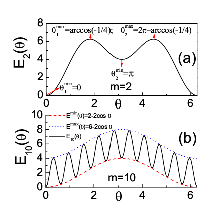
Fig. 2 shows versus for (a) and (b). We note that is an oscillatory function, and there are more regular oscillations for large values of . The number of maxima (or minima) of in the range is . As we will show, these extreme points give contributions to the integrals when we calculate the classical and quantum efficiency in Eqs. (15) and (16).
IV.2 Efficiency and scaling of the classical and quantum transport
In this subsection, we consider the efficiency of the classical and quantum transport. We calculate the integrals of Eqs. (15) and (16) using the stationary phase approximation (SPA) (See Appendix A). We find that the classical and quantum return probabilities show different scaling behavior for small values and large values of .

For small values of , we get an asymptotical expression for the classical ,
| (17) |
(See derivation in Appendix B). For large values of , we also get an approximate result (See Appendix B),
| (18) |
We note that scales as for small values of , however, for large , the scaling becomes as .
Quantum mechanically, we also find different scaling behavior of for small value and large value of . For small values of , is an oscillatory function multiplied by (See Eq. (30) in Appendix C for ). For large values of , there is an approximate result given by Eq. (37) in Appendix C,
| (19) |
Therefore, quantum transport of small displays the same scaling behavior while transport of large shows scaling . It is interesting to note that, both for the classical and quantum transport, the scaling exponent for large is twice the exponent for small values of . This is one of the main conclusions in this paper.
In order to test the theoretical predictions, Fig. 3 shows the classical and quantum return probabilities for LRICs of with , and . Fig. 3 (a) shows the classical return probability. We note that and displays the same scaling , but for the scaling becomes . The results are in good agreement with the analytical predictions of Eqs. (17) and (18). Fig. 3 (b) shows the quantum for and the analytical prediction of Eq. (30) in Appendix C. Both the results exhibit power law . The same scaling behavior () is also observed for (See Fig. 3 (c)). In Fig. 3 (d), we show and the analytical result predicted by Eq. (19). Both the results display the same scaling .
IV.3 Long time averages on finite networks


In this section, we consider the long time averaged transition probabilities on finite networks. Classically, the long time liming probabilities equal to the equip-partitioned probability [23]. Quantum mechanically, the long time averages of the transition probabilities does not lead to equip-partition. For LRICs, the long-time averaged probability is determined by Eq. (11) but the distribution patterns are complex for different network parameters and . For the cycle graph (nearest neighboring lattice), the limiting probability distribution depends on the parity of the network size . Fig. 4 shows the distribution patterns of the limiting transition probability on networks of with various values of . The initial excitation is located at node . As we can see, there are high probabilities to find the exciton at the initial node and the opposite node , this feature is a natural consequence of the periodic boundary condition of the graphs [20]. For odd-numbered networks , there is a higher probability to find the initial node than that at other nodes [20]. Fig. 5 shows the distribution patterns for networks of with various . The patterns depend on the specific network parameters and there are high probabilities to find the exciton at some particular nodes. We also note that the patterns of are the same for some different values of , this feature can be explained by the identical degeneracy distribution of the eigenvalues for different values of [20].

It is worth mentioning that for even-numbered networks, there are high probabilities to find the exciton at the initial node and opposite node. For networks of , we find the two probabilities are exactly equal to each other for all the values of , i.e., . However, for some other even-numbered network size , this is not true [20]. For some particular values of and , for instance and , the probability of finding the exciton at the initial node differs from the probability of the finding the exciton at the opposite node. Such asymmetry is small and not easy to be observed from the limiting probability distributions [20]. To detect such asymmetry of the probabilities, we define the quantity as a function of the network size for different values of [20]. The asymmetry is indicated by the nonzero of this quantity while corresponds to identical values of and . A plot of versus for , and are shown in Fig. 6. We find that the points break into several clusters, whereas some clusters decreases with the network size as a power law: [20].
V trapping on LRICs
An important process related to random walk is trapping [24, 25]. Trapping problems have been widely studied in the frame of physical chemistry, as part of the general reaction-diffusion scheme [26]. Previous work has been devoted to the trapping problem on discrete-time random walks [27, 28]. However, even in its simplest form, trapping was shown to yield a rich diversity of results, with varying behavior over different geometries, dimension, and time regimes [28]. The main physical quantity related to trapping process is the survival probability, which denotes the probability that a particle survives during the walk in a space with traps.
In this paper, we consider trapping using the approach based on time dependent perturbation theory and adopt the methodology proposed in Ref. [29]. In Ref. [29], the authors consider a system of nodes and among them are traps (). The trapped nodes are denoted them by , so that . The new Hamiltonian of the system is , where is the original Hamiltonian without traps and is the trapping operator. has purely imaginary diagonal elements at the trap nodes and assumed to be equal for all (). See Ref. [29] for details. The new Hamiltonian is non-hermitian and has complex eigenvalues and eigenstates {, } (). Then the quantum transition probability is
| (20) |
where () is the conjugate eigenstates of the new Hamiltonian. In order to calculate , all the complex eigenvalues and eigenstates {, } () are required. Here, we numerically calculate by diagonalizing the Hamiltonian H using the standard software package Mathematica 5.0.
Equation (20) depends on the initially excited node . The average survival probability over all initial nodes and all final nodes , neither of them being a trap node, is given by,
| (21) |
For continuous-time random walks (CTRWs), we induce trapping analogously as the CTQWs, where the new transfer matrix is modified by the trapping matrix as . The mean survival probability analogous to Eq. (21) is [29].

Fig. 7 shows the quantum and classical survival probabilities on LRICs of with , and . Five trapped nodes are randomly selected from all the nodes and is fixed in the numerical calculation. For each specific trapping configuration, we calculate the survival probability and average it over different configurations. As we can see from Fig. 7, both the quantum and classical survival probabilities decays fast on LRICs with large values of . This is opposite to the case in Ref. [30] where long-range interaction leads to a slower trapping of the excitation.
VI Conclusions and Discussions
We have studied coherent exciton dynamics modeled by continuous-time quantum walks (CTQWs) on long-range interacting cycles (LRICs). We have shown that both the efficiency of the classical and quantum transport display power laws, and the exponents for LRICs with large values of are twice the exponents of LRICs with small values of . Theoretical calculation of the return probability using stationary phase approximation supports this finding. In the long time limit, the limiting probability distributions of quantum transport show various patterns on finite size networks. When the network size is an even number, we find an asymmetric transition probability between the initial node and its opposite node. This asymmetry depends on the precise values of and . Finally, we study trapping process on LRICs and find that long-range interaction (large ) leads to a fast decay of the survival probability.
It is worth mentioning that the return probability displays different scaling behavior for small values and large values of . However, we did not give a quantitative relation between the scaling exponent and the parameter . We only know the scaling behavior for the thresholds of small and large , the scaling behavior in the medial region of is still unknown. In addition, the limiting probability distributions show various patterns on finite size networks. These patterns is a natural result of the interference phenomena in coherent transport on finite systems. The asymmetry of the limiting probability on even-numbered networks is also an interesting and strange feature of quantum walks, which deserves our further investigation [23, 31]. The long-range interaction in LRICs leads to a fast exciton trapping and is opposite to the conclusions in Ref. [30]. We also note that the quantum return probability in Ref. [18] scales the same behavior for various long-range interactions (). The different behavior of trapping and transport efficiency may be caused by the distinct type of long-range interactions.
Acknowledgements.
We thank Prof. Blumen (University of Freiburg) for useful discussions. This work is supported by National Natural Science Foundation of China under projects 10575042, 10775058 and MOE of China under contract number IRT0624 (CCNU).Appendix A The stationary phase approximation (SPA)
Stationary phase approximation (SPA) is an approach for solving integrals analytically by evaluating the integrands in regions where they contribute the most [32, 18, 10]. This method is specifically directed to evaluating oscillatory integrands, where the phase function of the integrand is multiplied by a relatively high value. Suppose we want to evaluate the behavior of function for large ,
| (22) |
The SPA asserts that the main contribution to this integral comes from those points where is stationary . If there is only one point for which and , the integral is approximated asymptotically by,
| (23) |
If there are more than one stationary points satisfy , then the integral is approximately given by the sum of the contributions [each being of the form given in Eq. (23)] of all the stationary points [18].
Appendix B Calculation of the classical using SPA
We apply SPA to calculate the classical in Eq. (15). The stationary points of this integral satisfy . The number of stationary points equals to ( maxima and minima, see Fig. 2) in the range . We denote maxima stationary points as () and minima stationary points as (). Then the integral of Eq. (15) yields,
| (24) |
which is mainly determined by the small values of . Considering , contributions from the maximal stationary points in the above equation is negligible. Therefore, can be simplified as,
| (25) |
For small values of , the global minimum at is sufficiently separated from (smaller than) other local minima. The sum in Eq. (25) is mainly from the contribution at the global minimum , thus,
| (26) |
Substituting the relation and into Eq. (26), we get,
| (27) |
For large values of , the global minimum at is not sufficiently separated from (smaller than) other local minima. The sum in Eq. (25) contains contributions from all the minimal stationary points. Noting that for large values of , the stationary points and are approximately equidistant, i.e., , (). Therefore, we get the approximations: , . Thus Eq. (25) can be written as,
| (28) |
where . In the continuum limit of large , equals to the integral , where (See the dashed curves in Fig. 2 (b)). We apply the method of SPA again to evaluate this integral and find that the contribution is mainly from the stationary point , which lead to . The classical of Eq. (28) transforms into,
| (29) |
Appendix C Calculation of the quantum using SPA
We calculate the integral of quantum return probability in Eq. (16). We also find the integral displays different scaling behavior for small values and large values of .
For small values of , we consider the case , where there are four stationary points: , , , (See Fig. 2 (a)). The second-order derivations at these points yield , and . The corresponding spectral eigenvalues at the four points are , and . Using the method of SPA, we obtain the integral of Eq. (16) for as,
| (30) |
Therefore, the quantum mechanical efficiency scales as for . For other small values of , the calculation is analogous. The result is also an oscillatory function multiplied by . This suggests that the quantum transport of small displays the same scaling behavior .
For the case of large , the integral of Eq. (16) comes from stationary points,
| (31) |
where in the last approximation and is applied. In the continuum limit of , the sum in the above equation can be written as the integral form,
| (32) |
and
| (33) |
Noting that and (See the dashed curves in Fig. 2 (b)), Eq. (31) can be rewritten as,
| (34) |
For the two integrals in the above equation, we apply SPA again and find that the contribution of this integral is mainly from two stationary points and . Thus
| (35) |
and
| (36) |
Substituting these relations into the Eq. (34), we get,
| (37) |
References
- [1] G. H. Weiss, Aspect and Applications of the Random Walk (North-Holland, Amsterdam, 1994).
- [2] J. Kempe, Contemp. Phys. 44, 307 (2002).
- [3] D. Supriyo, Quantum Transport: Atom to Transistor (Cambridge University Press, London, 2005).
- [4] R. Metzler und J. Klafter, Phys. Rep. 339, 1 (2000).
- [5] B. J. Kim, H. Hong and M. Y. Choi, Phys. Rev. B 68, 014304 (2003).
- [6] F. W. Strauch, Phys. Rev. A 74, 030301R, (2006).
- [7] M. Varbanov, H. Krovi and T. A. Brun, Phys. Rev. A 78, 022324 (2008).
- [8] A. Ambainis, Int. J. Quantum Inf. 1, 507 (2003).
- [9] G. Abal, R. Siri, A. Romanelli, et al., Phys. Rev. A 73, 042302 (2006).
- [10] M. A. Jafarizadeh and S. Salimi, Ann. Phys. 322, 1005 (2007).
- [11] D. Solenov and L. Fedichkin, Phys. Rev. A 73, 012313 (2003)
- [12] H. Krovi and T. A. Brun, Phys. Rev. A 73, 032341 (2006).
- [13] O. Mülken and A. Blumen, Phys. Rev. E 71, 016101 (2005).
- [14] S. Salimi, Int. J. Quantum Inf. 6, 945 (2008).
- [15] O. Mülken, V. Bierbaum and A. Blumen, J. Chem. Phys 124, 124905 (2006).
- [16] N. Konno, Infin. Dimens. Anal. Quantum Probab. Relat. Top. 9, 287 (2006).
- [17] N. Konno, Int. J. Quantum Inf. 4, 1023 (2006).
- [18] O. Mülken, V. Bierbaum and A. Blumen, Phys. Rev. E 77, 021117 (2008).
- [19] X. P. Xu, W. Li and F. Liu , Phys. Rev. E 78, 052103 (2008).
- [20] X. P. Xu, Phys. Rev. E 77, 061127 (2008).
- [21] C. Kittel, Introduction to solid state physics (Wiley, New York, 1986).
- [22] O. Mülken and A. Blumen, Phys. Rev. E 73, 066117 (2006).
- [23] A. Volta, O. Mülken and A. Blumen, J. Phys. A 39, 14997 (2006).
- [24] M. D. Hatlee and J. J. Kozak, Phys. Rev. B 21, 1400 (1980).
- [25] T. C. Lubensky, Phys. Rev. A 30, 2657 (1984).
- [26] A. Blumen, J. Klafter, and G. Zumofen, Phys. Rev. B 28, 6112 (1983).
- [27] F. Jasch and A. Blumen, Phys. Rev. E 64, 066104 (2001).
- [28] L. K. Gallos, Phys. Rev. E 70, 046116 (2004).
- [29] O. Mülken, A. Blumen, T. Amthor, C. Giese, M. Reetz-Lamour and M. Weidemüller, Phys. Rev. Lett. 99, 090601 (2007).
- [30] O. Mülken, V. Pernice, and A. Blumen,Phys. Rev. E 78, 021115 (2008).
- [31] O. Mülken, A. Volta and A. Blumen, Phys. Rev. A 72, 042334 (2005).
- [32] C. M. Bender and S. A. Orszag, Advanced Mathematical Methods for Scientists and Engineers (McGraw-Hill, New York, 1978).