Brane inflation revisited after WMAP five-year results

Yin-Zhe Ma Email: yzm20@cam.ac.uk Affiliation: Institute of Astronomy, University of Cambridge, Madingley Road, Cambridge CB3 0HA, United Kingdom Xin Zhang Email: zhangxin@mail.neu.edu.cn Affiliation: College of Sciences, Northeastern University, Shenyang 110004, Liaoning, People’s Republic of China

Abstract

In this paper, we revisit brane inflation models with the WMAP five-year results. The WMAP five-year data favor a red-tilted power spectrum of primordial fluctuations at the level of two standard deviations, which is the same as the WMAP three-year result qualitatively, but quantitatively the spectral index is slightly greater than the three-year value. This result can bring impacts on brane inflation models. According to the WMAP five-year data, we find that the KKLMMT model can survive at the level of one standard deviation, and the fine-tuning of the parameter $\beta$ can be alleviated to a certain extent at the level of two standard deviations.

I Introduction

The inflation paradigm of the early universe provides a compelling explanation for many big puzzles in the standard big bang cosmology, such as the problems of homogeneity, isotropy and flatness of the universe [1]. This period of accelerated expansion in the early universe predicts a nearly scale-invariant perturbation power spectrum, which has already been supported by the measurement of temperature fluctuations in the cosmic microwave background radiation [2, 3]. In spite of many phenomenological successes of the inflation based on effective field theory, there exist serious problems, concerning the origin of the scalar field driving inflation, namely the singularity problem and the trans-Plankian problem. Therefore, it is expected that inflation should be realized in a more natural way from some fundamental theory of microscopic physics. String theory is one of the most promising candidates for the fundamental microscopic physics, so it is very important to try to embed the inflation scenarios into string theory. One possible inflation scenario within the framework of string theory is the brane inflation, in which the inflation is driven by the potential between the parallel dynamic brane and anti-brane [4, 5, 6]. The distance between the branes in the extra compactified dimensions plays the role of the inflaton field. However, generically, getting a sufficiently flat inflaton potential in brane inflation models is not an easy thing [6].

A rather realistic slow roll inflation scenario based on string theory was first proposed by Kachru et al. [7]. In [7], by introducing some $\overline{\rm D}$ 3-branes in a warped geometry in type IIB superstring theory to break supersymmetry, the authors successfully lift the AdS vacuum to a metastable de Sitter vacuum with sufficiently long lifetime. This mechanism is often called KKLT mechanism. Furthermore, by putting an extra pair of the brane and anti-brane in this scenario, one can successfully realize a slow roll inflation model, namely the KKLMMT model [8]. In this model, the anti-brane is fixed at the bottom of a warped throat, while the brane is mobile and experiences a small attractive force towards the anti-brane. The inflation ends when the brane and the anti-brane collide and annihilate, initiating the hot big bang epoch. The annihilation of the brane and anti-brane makes the universe settle down to the string vacuum state that describes our universe. During the process of the brane collision, cosmic strings are copiously produced [9, 10]. For a well-worked inflationary scenario, the production of topological defects other than cosmic strings must be suppressed by many orders of magnitude. For extensive studies on the KKLMMT model and other types of brane inflation models, see, e.g., [11, 12, 13, 14, 15, 16, 17, 18].

Recently, the WMAP team released the five-year data [19]. For the $\Lambda$ CDM model, WMAP five-year data show that the index of power spectrum satisfies¹¹ 1 The pivot scale is taken to be $k_{\rm pivot}=0.002{\rm Mpc}^{-1}$ .

n_{s}=0.963_{-0.015-0.028}^{+0.014+0.029}~~~(1\sigma,2\sigma~\text{CL});

(1)

combining WMAP with SDSS and SNIa, the result is

n_{s}=0.960_{-0.013-0.027}^{+0.014+0.026}~~~(1\sigma,2\sigma~\text{CL}),

(2)

which is a little bluer than the WMAP three-year result, though the red power spectrum is still favored at the level of $3\sigma$ CL. Meanwhile, the running of the spectral index is not favored anymore. With WMAP five-year data only, the running of the spectral index is²² 2 In this case, the result of the spectral index is $n_{s}=1.031^{+0.054}_{-0.055}$ .

\alpha_{s}=\frac{dn_{s}}{d\ln k}=-0.037_{-0.028}^{+0.028}~~~(1\sigma~\text{CL}).

(3)

combining with SDSS and SNIa data, the result is³³ 3 In this case, the result of the spectral index is $n_{s}=1.022^{+0.043}_{-0.042}$ .

\alpha_{s}=\frac{dn_{s}}{d\ln k}=-0.032_{-0.020}^{+0.021}~~~(1\sigma~\text{CL}).

(4)

It is notable that the result of the spectral index in five-year WMAP is slightly larger than that in three-year WMAP. More evidently, the result of the running of the spectral index in five-year WMAP is much smaller than that in three-year WMAP. Finally, let’s see the result of the amplitude of the primordial gravitational waves. When combining WMAP data with SDSS and SNIa data, the tensor-to-scalar ratio $r$ is limited under a much tighter bound:⁴⁴ 4 In this case, the result of the spectral index is $n_{s}=0.968\pm 0.015$ .

r<0.20~~~(95\%~\text{CL}).

(5)

Based on the WMAP three-year results, Huang et al. [13] investigated brane inflation models and showed that the KKLMMT model cannot fit WMAP+SDSS data at the level of one standard deviation and a fine-tuning (at least eight parts in a thousand) is needed at the level of two standard deviations. Now, the WMAP data are updated to the five-year ones, so it is meaningful to see how the status of brane inflation is affected by the arrival of the new WMAP data. Therefore, in this paper, we address this issue, i.e., we revisit brane inflation with the WMAP five-year results.

This paper is organized as follows: In section II, we discuss a simple brane inflation model neglecting the problem of dynamic stabilization. In section III, we focus on the KKLMMT model and investigate to what degree the model is fine-tuned under the WMAP five-year data. The conclusion is given in the last section.

II A general brane Inflation model

First, let’s consider some general brane inflation models. Consider a pair of $Dp$ and $\bar{D}p$ -branes ( $p\geq 3$ ) filling the four large dimensions and separated from each other in the extra six dimensions that are compactified. The inflaton potential is given by [6, 13]

V=V_{0}\left(1-\frac{\mu^{n}}{\phi^{n}}\right),

(6)

where $V_{0}$ is an effective cosmological constant on the brane provided by brane tension, and the second term in (6) comes from the attractive force between the branes. The parameter $n$ satisfies the relation $n=d_{\perp}-2$ , where $d_{\perp}=9-p$ is the number of transverse dimensions. Obviously, we have $n\leq 4$ due to $d_{\perp}\leq 6$ . Corresponding to the $e$ -folding number $N$ before the end of inflation, the inflaton field $\phi$ takes the value

\phi_{N}=[NM_{pl}^{2}\mu^{n}n(n+2)]^{1/(n+2)},

(7)

where $M_{pl}$ is the reduced Planck mass of four dimensional world. The slow-roll parameters can be given as

\epsilon_{v}=\frac{M_{pl}^{2}}{2}\left(\frac{V^{\prime}}{V}\right)^{2}=\frac{n^{2}}{2(n(n+2))^{\frac{2(n+1)}{n+2}}}\left(\frac{\mu}{M_{pl}}\right)^{\frac{2n}{n+2}}N^{-\frac{2(n+1)}{n+2}},

(8)

\eta_{v}=M_{pl}^{2}\frac{V^{\prime\prime}}{V}=-\frac{n+1}{n+2}\frac{1}{N},

(9)

\xi_{v}=M_{pl}^{4}\frac{V^{\prime}V^{\prime\prime\prime}}{V^{2}}=\frac{n+1}{n+2}\frac{1}{N^{2}}.

(10)

Due to the fact that $\mu$ is much less than $M_{pl}$ , $\xi_{v}$ is negligible. Hence, the amplitude of the tensor perturbations is negligible [13]. One then obtains the spectral index and its running:

n_{s}=1-\frac{n+1}{n+2}\frac{2}{N},

(11)

\alpha_{s}=-\frac{n+1}{n+2}\frac{2}{N^{2}}.

(12)

It is easy to see that the running of the spectral index $\alpha_{s}$ is also negligible.

Refer to caption — Figure 1: Comparison of the WMAP five-year results of the special index with the brane inflation model. Note that since the number of the brane transverse dimensions is not greater than $6$ , the region with $n>4$ is not allowed (yellow region). Left: WMAP five-year results only; right: WMAP five-year data combined with SNIa and BAO data.

Figure 1 shows the spectral index for different parameter $n$ and $e$ -folding number $N$ . The region of $n>4$ is not allowed by theory, since the number of transverse dimensions is less than six. We focus on the two cases of $n=2$ and 4 corresponding respectively to the $D5$ and $D3$ -brane cases. From Fig. 1, we see that the brane inflation model is consistent with the WMAP data within some range of $N$ . On the other hand, it has been proposed in [21] that the $e$ -folding number relevant to observations should be

N=54\pm 7.

(13)

So, we shall check whether the fitting of WMAP five-year data can give a reasonable $e$ -folding number consistent with the result of (13), namely, $47<N<61$ .

Table 1: Fitting results for the number of

e

-folds

N

Model	WMAP5 Only	WMAP5+SNIa+BAO	WMAP5+ACBAR	WMAP5+CMB⁵⁵ 5 This includes the small-scale CMB measurements from CBI, VSA, ACBAR and BOOMERanG, see [19, 20, 23].
$D5$ -brane ( $n=2$ )	$N=40.5^{+24.7+147.0}_{-29.4-23.1}$	$N=37.5^{+20.2+69.6}_{-9.2-15.1}$	$N=41.7^{+26.5+145.8}_{-11.7-17.9}$	$N=37.5^{+20.2+77.9}_{-9.7-15.1}$
$D3$ -brane ( $n=4$ )	$N=45.0^{+27.5+163.3}_{-12.9-19.4}$	$N=41.7^{+22.4+77.3}_{-10.3-16.8}$	$N=46.3^{+29.5+162.0}_{-13.0-19.8}$	$N=41.7^{+22.4+86.5}_{-10.8-16.8}$

Table 1 is the result of the fitting to the WMAP data (combined with other observational data) for the number of $e$ -folds $N$ . It is clear to see that the fitting values of the $e$ -folding number are generally consistent with the result of [21], $N=47\sim 61$ , within $1\sigma$ range. Therefore, testing with the WMAP five-year data, one finds that the model survives at the level of 1 $\sigma$ .

Furthermore, let us consider the running of the spectral index. We plot $\alpha_{s}$ vs. $N$ in Fig. 2. From the left panel of this figure, we find that though the brane inflation model cannot yield the right results of the running of the spectral index given by WMAP five-year data in 1 $\sigma$ range with a reasonable $e$ -folding number, but it can be consistent with the observational results in 2 $\sigma$ range. From the right panel of Fig. 2, one finds that, for WMAP5+SN+BAO, the model is even consistent with the data in 1 $\sigma$ range. Fig. 3 shows the joint two-dimensional marginalized distribution of the spectral index $n_{s}$ and its running $\alpha_{s}$ , for WMAP five-year data. From this figure, we see that the trajectories of the brane inflation model (D5 and D3-brane cases) are within the region of 1 $\sigma$ CL.

By modifying the CAMB code [22], we also compare the angular power spectrum of the model with the WMAP five-year data, see Fig. 4. In the left panel, we see that the angular power spectrum produced by the model is generally consistent with the WMAP five-year data, although the cases with $n=2$ and $n=4$ have little greater amplitudes of the low multipole moments (basically quadrupole and octopole) compared with the best fit of the WMAP five-year data. However, due to the cosmic variance and statistical errors, the low multipole moments have large error bars, the model prediction is consistent with the observational data.

The above analyses show that the general brane inflation model can survive confronting the WMAP five-year data. When considering the WMAP five-year result of the spectral index, the model survives at the level of 1 $\sigma$ . This conclusion is different from that of the analysis of WMAP three year data. It was indicated in [13] that, with the WMAP three year data, the brane inflation model for $n=4$ is near the boundary of the WMAP3 only and cannot fit the WMAP3+SDSS data at the level of 1 $\sigma$ ; the case with $n=2$ is outside the range allowed by WMAP3 only or WMAP3+SDSS at the level of 1 $\sigma$ . So, we find that the WMAP five-year data save the brane inflation model to the level of 1 $\sigma$ .

However, the brane inflation model discussed above is not a realistic model. An important problem is neglected in the above discussions, which is that the distance between the brane and the anti-brane must be larger than the size of the extra dimensional space if the inflation is slow rolling (or $\eta$ is sufficiently small) in this scenario. Of course, there may exist such a possibility that the potential in (6) can emerge in other theories that we do not know currently, as pointed out in [13]. The first realistic brane inflation model is the so-called KKLMMT model [8] that will be discussed in the subsequent section.

III The KKLMMT model

The KKLMMT model is set up in the type IIB string theory. In this model, the highly warped compactifications are considered, with all moduli stabilized by the combination of fluxes and non-perturbative effects [8]. Once a small number of $\overline{\rm D}$ 3-branes are added, the vacuum can be successfully lifted to dS. Furthermore, one can add an extra pair of D3-bane and $\overline{\rm D}$ 3-brane in a warped throat, with the D3-brane moving towards the $\overline{\rm D}$ 3-brane that is located at the bottom of the throat. The scenario of brane inflation can thus be realized. The warped geometry successfully solves the $\eta$ problem, i.e., it can provide a natural mechanism for achieving a sufficiently flat potential. In this section, we shall discuss the KKLMMT model with the WMAP five-year results.

III.1 The setup and theoretical results

Consider a type IIB orientifold compactified on a Calabi-Yau 3-fold with fluxes, where all moduli are stabilized [11, 12]. Inside the bulk of the Calabi-Yau manifold, there are throats with warped geometry, where the metric has the approximate $AdS_{5}\times S_{5}$ form, where $X_{5}$ is some orbifold of $S_{5}$ and the $AdS_{5}$ metric in Poincare coordinates has the form [11, 12]

ds^{2}=h^{-\frac{1}{2}}(r)(-dt^{2}+a(t)^{2}d\vec{x}^{2})+h^{\frac{1}{2}}(r)ds_{6}^{2},

(14)

where the $h(r)$ is the warp factor

h(r)=\frac{R^{4}}{r^{4}},

(15)

in which $R$ is the radius of curvature of the $AdS_{5}$ throat. Following [11, 13], we consider the potential for the KKLMMT model given by

V(\phi)=\frac{1}{2}\beta H^{2}\phi^{2}+2T_{3}h^{4}(1-\frac{\mu^{4}}{\phi^{4}}),

(16)

where $T_{3}$ is the D3-brane tension and we have the relation $\mu^{4}=\frac{27}{32\pi^{2}}T_{3}h^{4}$ . Then we have

V(\phi)=\frac{1}{2}\beta H^{2}\phi^{2}+\frac{64\pi^{2}\mu^{4}}{27}(1-\frac{\mu^{4}}{\phi^{4}}).

(17)

So the derivative of this potential is

V^{\prime}(\phi)=\beta H^{2}\phi+\frac{256\pi^{2}\mu^{8}}{27}\frac{1}{\phi^{5}}.

(18)

Under the slow roll approximation, we have the Friedmann equation

3M_{pl}^{2}H^{2}\simeq V(\phi)\simeq V_{0}=\frac{64\pi^{2}\mu^{4}}{27},

(19)

which leads to the approximation relation $H^{2}=\frac{64\pi^{2}\mu^{4}}{27\times 3M_{pl}^{2}}$ we will use in the following calculation.

The procedure to obtain the inflaton field value at the moment of the $e$ -folding number $N$ before the end of inflation is as follows: First, we get the inflaton field value at the end of inflation by using the condition $\eta=-1$ ; then, we use the definition of $e$ -folding number $N=\int Hdt$ to obtain the field value at the moment corresponding to the e-folding number $N$ . Therefore, we first calculate the slow-roll parameter $\eta$ :

\eta=M_{pl}^{2}(\frac{V^{\prime\prime}}{V})\simeq M_{pl}^{2}(\frac{V^{\prime\prime}}{V_{0}}),

(20)

where

V^{\prime\prime}=\beta H^{2}-\frac{1280\pi^{2}\mu^{8}}{27}\phi^{-6}.

(21)

Substituting $H^{2}=\frac{64\pi^{2}\mu^{4}}{27\times 3M_{pl}^{2}}$ into the above equation, we obtain

\eta=\frac{\beta}{3}-20\mu^{4}M_{pl}^{2}\frac{1}{\phi^{6}}.

(22)

Thus, the field value at the end of inflation $\phi_{f}$ satisfies

-1=\frac{\beta}{3}-20\mu^{4}M_{pl}^{2}\frac{1}{\phi_{f}^{6}},

(23)

and we obtain

\phi_{f}^{6}=\frac{20\mu^{4}M_{pl}^{2}}{1+\frac{\beta}{3}}.

(24)

Under the slow roll approximation, we have

$\displaystyle N$	$\displaystyle=$	$\displaystyle\int_{\phi_{f}}^{\phi_{N}}dN=(3H^{2})\int_{\phi_{f}}^{\phi_{N}}\frac{d\phi}{V^{\prime}(\phi)}$
	$\displaystyle=$	$\displaystyle(3H^{2})\int_{\phi_{f}}^{\phi_{N}}\frac{d\phi}{\beta H^{2}\phi+\frac{256\pi^{2}\mu^{8}}{27}\frac{1}{\phi^{5}}}$
	$\displaystyle=$	$\displaystyle\frac{1}{2\beta}\ln\left[256\pi^{2}\mu^{8}+27H^{2}\beta\phi^{6}\right]_{\phi_{f}}^{\phi_{N}}.$

Substituting $H^{2}=\frac{64\pi^{2}\mu^{4}}{27\times 3M_{pl}^{2}}$ and Eq. (24) into the above equation, we obtain

	$\displaystyle\phi_{N}^{6}$	$\displaystyle=$	$\displaystyle e^{2\beta N}\phi_{f}^{6}+\frac{12M_{pl}^{2}}{\beta}\mu^{4}(e^{2\beta N}-1)$		(25)
		$\displaystyle=$	$\displaystyle 24M_{pl}^{2}\mu^{4}[\frac{e^{2\beta N}(1+2\beta)-(1+\frac{1}{3}\beta)}{2\beta(1+\frac{1}{3}\beta)}],$		(25)

\phi_{N}^{6}=24M_{pl}^{2}\mu^{4}m(\beta),

(26)

where

m(\beta)=\frac{e^{2\beta N}(1+2\beta)-(1+\frac{1}{3}\beta)}{2\beta(1+\frac{1}{3}\beta)}.

(27)

With the value of $\phi_{N}$ , we can write

\epsilon_{v}=\frac{1}{18}\left(\frac{\phi_{N}}{M_{pl}}\right)^{2}\left[\beta+\frac{1}{2m(\beta)}\right]^{2},

(28)

\eta_{v}=\frac{\beta}{3}-\frac{5}{6}\frac{1}{m(\beta)},

(29)

\xi_{v}=\frac{5}{3}\frac{1}{m(\beta)}\left[\beta+\frac{1}{2m(\beta)}\right].

(30)

The amplitude of the scalar comoving curvature fluctuations has been given in [11, 13]:

\Delta_{\cal R}^{2}\simeq\frac{V}{M_{pl}^{4}}\frac{1}{24\pi^{2}\epsilon_{v}}=\frac{2}{27m(\beta)}\left(\beta+\frac{1}{2m(\beta)}\right)^{-2}\left(\frac{\phi_{N}}{M_{pl}}\right)^{4},

(31)

thus we have

\frac{\phi_{N}}{M_{pl}}=(\frac{27}{8})^{\frac{1}{4}}m(\beta)^{-\frac{1}{4}}(1+2\beta m(\beta))^{\frac{1}{2}}(\Delta_{\cal R}^{2})^{\frac{1}{4}}.

(32)

Substituting the above equation into Eq. (28), we have the following expression for $\epsilon_{v}$ :

\epsilon_{v}=\frac{1}{48}\left(\frac{3}{2}\right)^{\frac{1}{2}}(\Delta_{\cal R}^{2})^{\frac{1}{2}}m(\beta)^{-\frac{5}{2}}(1+2\beta m(\beta))^{3}.

(33)

The WMAP five-year data give the amplitude of the primordial scalar power spectrum, $\Delta_{\cal R}^{2}\simeq 2.4\times 10^{-9}$ for $N\sim 50$ [19, 20]. Thus, so far, all of the slow roll parameters can be expressed as the functions of $\beta$ (and $N$ ). The spectral index and its running are

n_{s}=1-6\epsilon_{v}+2\eta_{v},~~~\alpha_{s}=-24\epsilon_{v}^{2}+16\epsilon_{v}\eta_{v}-2\xi_{v},

(34)

and the tensor-to-scalar ratio is

r=16\epsilon_{v}.

(35)

III.2 What can observables tell us?

Inflation models can predict some observables, such as the spectral index, its running, and the tensor-to-scalar ratio, etc., from which one can link the observations to the theory. In particular, the brane inflation models also predict the existence of cosmic superstrings that open a significant window for testing the superstring theory. In this subsection, we shall discuss how these observables provide constraints on the parameter $\beta$ of the KKLMMT model.

III.2.1 Tensor-to-scalar ratio

First, let’s discuss the tensor-to-scalar ratio $r$ . The tensor-to-scalar ratio is an important observable that can distinguish the inflationary cosmology from other scenarios. Also, it can be used to distinguish different inflation models because different models give distinctive predictions on this observable quantity. Although the observations still have no ability to detect the primordial gravitational waves in a convincing manner, an upper limit could be given at least. Now we try to see how this observable with such a loose upper-limit can set constraint on the KKLMMT model. In Fig. 5, we plot the tensor-to-scalar ratio $r$ vs. the $e$ -folding number $N$ for the KKLMMT model, according to Eq. (35).

In Fig. 5, we see that the larger value the parameter $\beta$ takes, the greater value the tensor-to-scalar ratio will be. This is due to the fact that the greater the value of $\beta$ is, the faster the inflaton moves, so the larger tensor mode will be produced in the inflationary era [24]. Currently, the tightest constraint on $r$ is $r<0.2$ (WMAP5+SNIa+BAO) [19, 20]. From Fig. 5 we see that the green curve (corresponding to $\beta=0.2$ ) definitely violates this bound, and we learn that the parameter $\beta$ cannot be greater than $0.15$ . Hence, we find that even such a loose bound on $r$ gives a so small value of $\beta$ about ${\cal O}(10^{-1})$ , then the true value of $\beta$ must be fine-tuned to some extent. We hope the future CMB experiments could further constrain $r$ toward $0.01$ , providing true test on the KKLMMT model.

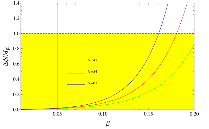
The above constraint on $\beta$ can also be examined from the field value perspective. We can calculate the change magnitude of the inflaton field from the moment when the fluctuations were generated to the end of inflation,

	$\displaystyle\frac{\Delta\phi}{M_{pl}}$	$\displaystyle=$	$\displaystyle\frac{\phi_{N}-\phi_{f}}{M_{pl}}$		(36)
		$\displaystyle=$	$\displaystyle\frac{3^{\frac{7}{12}}}{2^{\frac{5}{4}}}m(\beta)^{-\frac{5}{12}}(1+2\beta m(\beta))^{\frac{1}{2}}(\Delta_{\cal R}^{2})^{\frac{1}{4}}\left[(24m(\beta))^{{1/6}}-\left(\frac{20}{1+{\beta/3}}\right)^{{1/6}}\right].$		(36)

According to [25], for a single field inflation model, the change magnitude of the field has a relationship with the tensor-to-scale ratio as

\frac{\Delta\phi}{M_{pl}}\geq\left(\frac{r}{0.01}\right)^{\frac{1}{2}}.

(37)

We plot the change magnitude of the field as a function of $\beta$ for different e-folding number $N$ in the left panel of Fig. 6. It is very explicit that if $\beta\geq 0.2$ , the change magnitude of the field will be definitely greater than the planck mass, which might not be consistent with the conditions of effective field theory [26, 27]. The right panel of Fig. 6 shows the allowed values for the parameter $\beta$ . According to Eq. (37), if the change of the field during the whole period of inflation is less than the Planck mass, the tensor-to-scalar ratio will be surely less than $0.01$ . Thus, from right panel of Fig. 6, it can be inferred that $\beta$ should be less than $0.17$ . Therefore, to satisfy the current constraint on the tensor-to-scalar ratio and the physical bound on the change magnitude of the field value, $\Delta\phi\leq M_{pl}$ , the parameter $\beta$ could not be greater than $0.15$ , which is both an observational and a physical bound on the KKLMMT model.

III.2.2 Cosmic string tension

Cosmic strings and other topological defects have long been proposed as one of the candidates for the origin of structure formation [28], however, it has been shown that this scenario leads to predictions incompatible with observations such as the power spectrum of cosmic microwave background (CMB) temperature anisotropy [29]. Nevertheless, the brane/anti-brane inflation scenario inspired from string theory naturally indicates that cosmic strings would have a small contribution to the CMB, which is compatible with the observational limits [9, 10, 15]. This has led to a significant revival of all aspects of cosmic string scenario, including new theoretical motivations, phenomenological implications and direct observational searches, see e.g. [11, 30, 31, 32, 33]. The possibility of detecting the signal of the cosmic strings through astronomical observations opens a significant window to test string theory. The current observational bound (the upper limit) for cosmic string tension from the CMB temperature is roughly [33]

G\mu_{\mathrm{obs}}\lesssim 1.8\times 10^{-7}\text{ }(1\sigma\text{ CL}),

(38)

and

G\mu_{\mathrm{obs}}\lesssim 2.7\times 10^{-7}\text{ (}2\sigma\text{ CL)}.

(39)

Obviously, the KKLMMT scenario predicts that the tension of these cosmic strings is very small and their contribution to CMB is well below the current limits [11, 32]. However, now, we try to do this inversely, i.e., we intend to see how this observational bound puts a constraint on the parameter $\beta$ . This may show what the loosest observational result can tell us.

The $D3$ -brane collides with the $\bar{D}3$ -brane at the end of inflation at the bottom of the throat. The annihilation of the D3- $\overline{\rm D}3$ -branes initiates the hot big bang epoch, meanwhile D1-branes (i.e. D-strings) and fundamental closed strings (i.e. F-strings) are also produced. The quantities of interest are the D-string tension $G\mu_{D}$ and the F-string tension $G\mu_{F}$ , where $\mu_{D}$ and $\mu_{F}$ are the effective tensions measured from the viewpoint of the four dimensional effective action. Since in ten dimensions, there is the relationship $T_{3}=T_{F}^{2}/2\pi g_{s}=T_{D}^{2}g_{s}/2\pi$ , where $T_{3}=1/(2\pi)^{3}g_{s}\alpha^{\prime 2}$ is the D3-brane tension, we have the tensions of the type IIB string in the inflationary throat

G\mu_{F}=GT_{F}h^{2}=\sqrt{\frac{g_{s}}{32\pi}}\left({\frac{T_{3}h^{4}}{M_{\mathrm{pl}}^{4}}}\right)^{1/2},

(40)

G\mu_{D}=GT_{D}h^{2}=\sqrt{\frac{1}{32\pi g_{s}}}\left({\frac{T_{3}h^{4}}{M_{\mathrm{pl}}^{4}}}\right)^{1/2},

(41)

where $g_{s}$ is the string coupling. There are also bound states of $p$ F-strings and $q$ D-strings with a cosmic string network spectrum [30]

\mu_{(p,q)}=\mu_{F}\sqrt{p^{2}+q^{2}/g_{s}^{2}}.

(42)

In Eqs. (40) and (41) both F-strings and D-strings are dependent on the string coupling $g_{s}$ , but the geometric mean $(\mu_{F}\mu_{D})^{1/2}$ is independent of $g_{s}$ . Thus, we can define [15]

G\mu_{s}=G(\mu_{F}\mu_{D})^{1/2}=\sqrt{\frac{1}{32\pi}}\left({\frac{T_{3}h^{4}}{M_{\mathrm{pl}}^{4}}}\right)^{1/2}.

(43)

Obviously, for F-string we have $\mu_{F}=\mu_{s}\sqrt{g_{s}}$ , and for D-string we have $\mu_{D}=\mu_{s}/\sqrt{g_{s}}$ . The value of $g_{s}$ is likely in the range 0.1 to 1 [30]. Note that $g_{s}>1$ can be converted to $g_{s}<1$ by $S$ -duality.

Then, combining with COBE normalization (31), we obtain the cosmic string tension in the KKLMMT inflation model

\displaystyle G\mu_{s}=\frac{1}{18}(\frac{\pi}{3})^{\frac{1}{2}}(\frac{27}{8})^{\frac{3}{4}}m(\beta)^{-\frac{5}{4}}(1+2\beta m(\beta))^{\frac{3}{2}}(\Delta_{\cal R}^{2})^{\frac{3}{4}}.

(44)

Equation (44) shows that the cosmic string tension $G\mu_{s}$ depends both on the parameter $\beta$ and the number of e-folds $N$ . Thus, in order to see how the cosmic string tension relies on the two parameters, we plot the correlation of $N$ - $\beta$ according to the cosmic string tension $G\mu_{s}$ in Fig. 7.

In Fig. 7, the upper-right corner is the not-allowed parameter region, since it represents a too large tension and it is excluded outside the $2\sigma$ CL. The smaller value the cosmic string tension takes, the deeper the curve will move toward the lower-left corner, which indicates a smaller parameter $\beta$ . According to the $1\sigma$ bound (the red curve in Fig. 7), if one takes $N=61$ , the observational $1\sigma$ curve will give the tightest constraint on $\beta$ , namely $\beta\lesssim 0.106$ ; if taking $N=47$ , the bound on the parameter $\beta$ from cosmic string tension will be looser, $\beta\lesssim 0.127$ . Thus, roughly speaking, the current observational bound on the cosmic string tension tells us the following information on the parameter $\beta$ , namely $\beta\lesssim 0.12$ .

III.2.3 Spectral index

The spectral index is certainly the most important observable that could distinguish different inflation models. The WMAP five-year data and the combination of various measurements favor a red power spectrum, which could put tight constraints on the KKLMMT model.

Now we plot the correlation of $r-n_{s}$ in the left panel of Fig. 8 to see what is the trajectory of the model when varying the parameter $\beta$ . In this figure, by decreasing the parameter $\beta$ , we show that the trajectory of the model goes from the upper-right corner to the lower-left corner in the $r-n_{s}$ plane. So, only $\beta\lesssim 0.01$ could give both the red-tilted scalar spectrum and the small field manner. This is due to the fact that a larger parameter $\beta$ will make the field rolling too fast, which might make the slow-roll parameter $\eta$ be positive. Therefore, the red-tilted power spectrum requires $\beta\lesssim 0.01$ . We also plot $\beta$ vs. $n_{s}$ for different number of e-folds $N$ in the right panel of Fig. 8. In this figure, it is easy to see that different number of $e$ -folds $N$ can make little influence on the curves, and the red-tilted spectrum roughly requires $\beta\lesssim 0.01$ .

Summarizing the above discussions, we see that the spectral index can put the tightest constraints on the KKLMMT model. This is obvious because the spectral index is the very quantity that has been precisely measured while other quantities only get loose upper limits from the observations. The aim of making these discussions is to see from various angles of view what constraints these observational quantities can bring to the model. From the above analysis, we get to know that the current observational bound on the parameter $\beta$ is roughly

\displaystyle\beta\lesssim{\cal O}(10^{-2}).

(45)

Further constraints from the WMAP five-year results will be discussed in the next subsection.

We now pause to discuss the physical effect of the parameter $\beta$ . If $\beta$ goes larger, the potential $V(\phi)$ will become steeper, which leads the inflaton to roll faster than the small $\beta$ case. Thus, the change magnitude of the inflaton field during inflation will be greater. At the same time, the $D3$ and $\bar{D}3$ -branes will have greater momentum to collide, producing more $D$ -strings and $F$ -strings. Therefore, constraining the parameter $\beta$ is actually constraining the shape of the potential and the dynamics of inflation.

III.3 Comparing to the WMAP five-year results

The WMAP three-year data give a rather red spectrum, i.e. $n_{s}=0.951^{+0.015}_{-0.019}$ (1 $\sigma$ CL) for WMAP3 data only, and $n_{s}=0.948^{+0.015}_{-0.018}$ (1 $\sigma$ CL) for the combination of WMAP3 and SDSS data. Therefore, such a red spectrum requires the parameter $\beta$ in the KKLMMT to be fine-tuned. In [13], it has been shown that, with the WMAP three-year data, the constraints on the parameter $\beta$ are $\beta\leq 6\times 10^{-4}$ at the level of 1 $\sigma$ and $\beta\leq 8\times 10^{-3}$ at the level of 2 $\sigma$ for WMAP3 only; $\beta\leq 6\times 10^{-3}$ at the level of 2 $\sigma$ for WMAP3 + SDSS. So, the fine-tuning for the parameter $\beta$ is needed, according to the constraints from the WMAP three-year results (see also [15]).

However, the scalar spectral index derived from the WMAP five-year data is relatively blue comparing to that of WMAP3, though it is still red-tilted. See Eqs. (1) and (2) for the results of WMAP5. Therefore, we expect that these results could relax the fine-tuning of $\beta$ to some extent.

We plot the spectral index $n_{s}$ as a function of the number of $e$ -folds $N$ in Fig. 9. For comparison, we also show the observational results of the spectral index, from the WMAP five-year data. In this figure, it is easy to see that the larger the parameter $\beta$ , the greater the spectral index. We also find that the curves are very sensitive to the parameter $\beta$ , i.e., the curves of the spectral index will change significantly even though the parameter $\beta$ only changes a little, e.g., from $0$ to $0.01$ . Note that $\beta<0$ is forbidden since in this case the $\beta$ term in the potential tends to push the D3-brane out of the throat such that the inflation will not happen. For the boundary curve corresponding to $\beta=0$ , the central value of $n_{s}$ gives a reasonable value of the $e$ -folding number $N$ ; however, when changing $\beta$ to $0.01$ , the model could not provide the central value of $n_{s}$ within its reasonable range of the number of $e$ -folds, which implies that the parameter $\beta$ tends to be fine-tuned confronting a red-tilted spectrum of the primordial perturbation.

Confronting the WMAP five-year results of the spectral index, Eqs. (1) and (2), the correlation between the parameter $\beta$ and the $e$ -folding number $N$ can also be derived, see Fig. 10. From this figure, one can clearly read off the allowed region in the parameter-space by the WMAP five-year data. Note that the area of $\beta>0$ and $47<N<61$ is a rational region for the KKLMMT model. Therefore, according to the WMAP five-year results of the spectral index, we see that the KKLMMT model can fit well with both the data of WMAP only and WMAP + BAO + SN within 1 $\sigma$ range. For WMAP only, we derive $\beta\leq 5.4\times 10^{-3}$ at the level of 1 $\sigma$ and $\beta\leq 1.4\times 10^{-2}$ at the level of 2 $\sigma$ . For WMAP + BAO + SN, we derive $\beta\leq 4.0\times 10^{-3}$ at the level of 1 $\sigma$ and $\beta\leq 1.0\times 10^{-2}$ at the level of 2 $\sigma$ . So, comparing to the WMAP five-year results, we find that the value of the parameter $\beta$ is relaxed to ${\cal O}(10^{-2})$ at the level of 2 $\sigma$ . The problem of fine-tuning of $\beta$ is alleviated to a certain extent when confronting the WMAP five-year data. This is, without doubt, a good news for the KKLMMT model.

For the running of the spectral index, according to the WMAP five-year data, one finds an upward shift from the three-year result, $\alpha_{s}=-0.032^{+0.021}_{-0.020}$ (WMAP5 + BAO + SN).⁶⁶ 6 Such a small value, $\alpha_{s}\sim-{\cal O}(10^{-2})$ , may indicate that there is no evidence for the running of the spectral index, as pointed out in [19]. The KKLMMT model, generally, cannot yield a seeable running of the spectral index. However, for $\beta>0.1$ , a large running is also possible in the KKLMMT model. Unfortunately, even though taking a big $\beta$ , the KKLMMT model cannot provide a running compatible with the current WMAP result for the running, see Fig. 11. Of course, the future high precision observations might make a more precise measure for the running of the spectral index, and might demonstrate explicitly that there is no running of the spectral index.

Furthermore, we also compare the angular power spectrum of the KKLMMT model with the WMAP five-year data, by employing the CAMB code [22], see Fig. 4. In the right panel of Fig. 4, we see that the smaller the value of $\beta$ is, the larger the first peak amplitude will be, and, obviously, $\beta=0.1$ is not able to fit the power spectrum at all. Thus, the current data of the CMB angular power spectrum also indicate that the parameter $\beta$ should be taken as $\lesssim 0.01$ , which is consistent with the constraint from the spectral index.

Finally, let’s discuss the prospects for the future measurements of the tensor-to-scalar ratio, $r$ , in light of the existing constraint on $n_{s}$ . From the above analysis, we know that the current constraints on $n_{s}$ put a bound on the KKLMMT model of order $\beta<0.01$ or so. Such a small value of $\beta$ leads to a negligible $r$ , less than ${\cal O}(10^{-5})$ , see Fig. 5. This means that if current bounds on $n_{s}$ do not shift appreciably, any observation of primordial tensor modes will rule out the KKLMMT model entirely. Therefore, the future measurements of $r$ might provide a disproof for the KKLMMT model.

IV Conclusion

In this paper, we have studied brane inflation with the WMAP five-year data. We first considered a general brane inflation model in which the problem of dynamic stabilization is neglected. Furthermore, we examined the KKLMMT model by using the WMAP five-year results.

For the general inflation model, we show that, according to the WMAP five-year data, the model survives at the level of 1 $\sigma$ . This conclusion is different from that of a previous work [13] which is based on the analysis of the WMAP three-year data. In [13], with the WMAP three-year data, it was indicated that the brane inflation model for $n=4$ (D3-brane case) is near the boundary of the WMAP3 only and cannot fit the WMAP3+SDSS data at the level of 1 $\sigma$ ; the model with $n=2$ (D5-brane case) is outside the range allowed by WMAP3 only or WMAP3+SDSS at the level of 1 $\sigma$ . Therefore, we find that the WMAP five-year data save the brane inflation model to the level of $1\sigma$ .

For the KKLMMT model, we first discuss how the various observables can bring constraints on the parameter $\beta$ of the model. Then, we compare the model to the WMAP five-year results. In [13], by using the WMAP three-year data, the authors find that the KKLMMT model cannot fit WMAP3+SDSS data at the level of 1 $\sigma$ and a fine-tuning, at least eight parts in a thousand, is needed at the level of 2 $\sigma$ . However, in this work, we show that the KKLMMT model is consistent with both the data of WMAP5 only and of WMAP5+BAO+SN at the level of $1\sigma$ . Moreover, comparing to the WMAP five-year results, we find that the value of the parameter $\beta$ is relaxed to ${\cal O}(10^{-2})$ at the level of 2 $\sigma$ . Therefore, the problem of fine-tuning of $\beta$ is alleviated to a certain extent when confronting the WMAP five-year data. This is definitely a good news for the KKLMMT model.

This paper only discusses the the simplest realistic brane inflationary model, namely the KKLMMT model, in which the usual slow-roll scenario is employed, but does not involve the Dirac-Born-Infeld (DBI) scenario, in which the rolling of the inflaton is albeit slow but relativistic. In the DBI model, large tensor mode and/or non-Gaussianity may emerge, providing a possible stringy signature. The DBI model has been investigated in detail in [18] by using the WMAP five-year data.

Acknowledgments

One of us (YZM) would like to thank Anne-Christine Davis, George Efstathiou, Hiranya Peiris, Qing-Guo Huang, Simeon Bird and Yi Wang for helpful discussions, also thank Duncan Hanson and Damien Quinn for computer help. This work was supported by grants from the Cambridge Overseas Trust and the studentship from Trinity College, Cambridge, and the Natural Science Foundation of China.

References

[1] A. H. Guth, Phys. Rev. D. 23 (1981) 347; A. D. Linde, Phys. Lett. B. 108 (1982) 389; A. Albrecht and P. J. Steinhardt, Phys. Rev. Lett. 48 (1982) 1220; for earlier attempts on an inflationary model, see, A. A. Starobinsky, Phys. Lett. B 91, 99 (1980).
[2] G. F. Smoot et al., Astrophys. J. 396 (1992) L1; C. L. Bennett et al., Astrophys. J. 464 (1996) L1, astro-ph/9601067.
[3] C. L. Bennett et al., Astrophys. J. Suppl. 148 (2003) 1, astro-ph/0302207; D. N. Spergel et al., Astrophys. J. Suppl. 148 (2003) 175, astro-ph/0302209; H. V. Peiris et al., Astrophys. J. Suppl. 148 (2003) 213, astro-ph/0302225.
[4] G. R. Dvali and S. H. Tye, Phys. Lett. B 450 (1999) 72, hep-ph/9812483.
[5] C. P. Burgess, M. Majumdar, D. Nolte, F. Quevedo, G. Rajesh and R. J. Zhang, JHEP 0107 (2001) 047, hep-th/0105204]; G. R. Dvali, Q. Shafi and S. Solganik, hep-th/0105203.
[6] F. Quevedo, Class. Quant. Grav. 19 (2002) 5721, hep-th/0210292.
[7] S. Kachru, R. Kallosh, A. Linde and S. P. Trivedi, Phys. Rev. D 68, 046005 (2003) [hep-th/0301240].
[8] S. Kachru, R. Kallosh, A. Linde, J. M. Maldacena, L. McAllister and S. P. Trivedi, JCAP 0310, (2003) 013, hep-th/0308055.
[9] N. T. Jones, H. Stoica and S. H. Tye, JHEP 0207, (2002) 051, hep-th/0203163.
[10] S. Sarangi and S. H. Tye, Phys. Lett. B 536, (2002) 185, hep-th/0204074.
[11] H. Firouzjahi and S.H. Tye, JCAP 0503 (2005) 009, hep-th/0501009.
[12] D. Baumann and L. McAllister, hep-th/0610285.
[13] Q. G. Huang, M. Li and J. H. She, JCAP 0611 (2006) 010, hep-th/0604186.
[14] Q. G. Huang, Phys. Rev. D 74, 063513 (2006) [arXiv:astro-ph/0605442].
[15] X. Zhang, JCAP 0612 (2006) 002, hep-th/0608207.
[16] R. Bean, S. E. Shandera, S. H. Henry Tye and J. Xu, JCAP 0705, 004 (2007) [arXiv:hep-th/0702107].
[17] L. Lorenz, J. Martin and C. Ringeval, JCAP 0804, 001 (2008) [arXiv:0709.3758 [hep-th]].
[18] L. Alabidi and J. E. Lidsey, Phys. Rev. D 78, 103519 (2008) [arXiv:0807.2181 [astro-ph]].
[19] E. Komastu et.al,astro-ph/0803.0547
[20] http://lambda.gsfc.nasa.gov/product/map/current/parameters.cfm
[21] L. Alabidi and D. H. Lyth, JCAP 0608 (2006) 013, astro-ph/0603539.
[22] http://camb.info; A. Lewis, A. Challinor and A. Lasenby, ApJ, 538 (2000) 473, astro-ph/9911177.
[23] B. S. Mason, et. al ApJ, 591 (2003) 540; J. L. Sievers, et. al, ApJ, 591 (2003) 599; J. L. Sievers, et. al ApJ, 660 (2007) 976; T. J. Pearson, et. al, ApJ, 591 (2003) 556; A. C. S. Readhead, et. al ApJ, 609 (2004) 498; C. Dickinson, et. al MNRAS, 353 (2004) 732; C. L. Kuo, et. al ApJ, 600 (2004) 32; C. L. Kuo, et. al ApJ, 664 (2007) 687; J. E. Ruhl, et. al ApJ, 599 (2003) 786; T. E. Montroy, et. al ApJ, 647 (2006) 813; F. Piacentini, et. al ApJ, 647 (2006) 833.
[24] D. Baumann, A. Dymarsky, S. Kachru, I. R. Klebanov, L. McAllister, hep-th/0808.2811
[25] D. H. Lyth, Phys. Rev. Lett. 78,(1997) 1861, [hep-ph/9606387]; G. Efstathiou and K. J. Mack, JCAP 0505,(2005) 008, [astro-ph/0503360]
[26] N. Arkani-Hamed, L. Motl, A. Nicolis and C. Vafa, JHEP 0706, 060 (2007) [arXiv:hep-th/0601001].
[27] Q. G. Huang, JHEP 0705, 096 (2007) [arXiv:hep-th/0703071].
[28] Y. B. Zeldovich, Mon. Not. Roy. Astron. Soc. 192 (1980) 663; A. Vilenkin, Phys. Rev. Lett. 46 (1981) 1169.
[29] U. L. Pen, U. Seljak and N. Turok, Phys. Rev. Lett. 79, (1997) 1611, astro-ph/9704165; B. Allen, R. R. Caldwell, S. Dodelson, L. Knox, E. P. S. Shellard and A. Stebbins, Phys. Rev. Lett. 79, (1997) 2624, astro-ph/9704160; A. Albrecht, R. A. Battye and J. Robinson, Phys. Rev. D 59 (1999) 023508, astro-ph/9711121.
[30] E. J. Copeland, R. C. Myers and J. Polchinski, JHEP 0406, 013 (2004) [arXiv:hep-th/0312067].
[31] M. G. Jackson, N. T. Jones and J. Polchinski, JHEP 0510, 013 (2005) [arXiv:hep-th/0405229].
[32] S. E. Shandera and S. H. Tye, JCAP 0605, 007 (2006) [arXiv:hep-th/0601099].
[33] M. Wyman, L. Pogosian and I. Wasserman, Phys. Rev. D. 72, (2005) 023513; M. Wyman, L. Pogosian and I. Wasserman, Phys. Rev. D. 73, (2006) 089905, Erratum, astro-ph/0503364; A. A. Fraisse, JCAP 03 (2007) 008, astro-ph/0603589; L. Pogosian, I. Wasserman and M. Wyman, astro-ph/0604141.