Electric field noise above surfaces: a model for heating rate scaling law in ion traps

In this work we present a model where we take explicitly into account the spatial dependence of the electric field noise density above a surface, introducing a characteristic length not yet considered in previous models: the correlation length, $\zeta$, of the noisy potential on the surface. In that picture, the noise arise from finite size sources distributed randomly on the surface. We show that this simple model accounts for the behavior of electric field noise scaling on the whole range covered by both ion heating measurements and cantilever-based measurements. We propose that this correlation length could be related to the characteristic size of the patches, opening a way to the control of noise intensity by engineering the material properties. In a recent work, an analytical solution of the Laplace equation for the special case of a planar ion trap was found[18]. In the present letter we extend this approach and obtain an analytical expression for the scaling law of the electric field noise density $S_{E}(\omega,d)$ at a distance $d$ of the surface. The first step is to solve the Laplace equation for the potential $\phi(x,y,z,t)$, $\Delta\phi(x,y,z,t)=0$ in half the space ($y>0$) with boundary condition $\phi(x,0,z,t)=\phi_{0}(x,z,t)$ and vanishing potential for $y\to\infty$. Under these assumptions, the potential reads:

where we took the Fourier transform of the Laplace equation, introducing $k_{x}$ and $k_{z}$. Then carrying out the integration on $k_{x}$ and $k_{z}$, the resulting potential above the plane is:

where we introduced $K(x,y,z)=\frac{y}{(x^{2}+y^{2}+z^{2})^{3/2}}$, the kernel of the Laplace problem with these specific boundary conditions. As in ref [18], equation (2) allows us to compute efficiently the potential associated to a given electrode geometry. More generally equation (2) allows us to compute the potential created by any disordered boundary condition $\phi_{0}(x,z,t)$.

In the following we will assume that small patch potentials distributed over the plane $(x,z)$ create a disordered electric potential on the surface. Let $\{C_{i}\}$ be the area of these patches and $V_{i}(t)$ the time-dependent electric noise on the patch $C_{i}$. With these notations one have: $\phi_{0}(x,z,t)=\sum_{i}V_{i}(t)\chi_{C_{i}}(x,z)$ where $\chi_{C_{i}}$ is the characteristic function of $C_{i}$ ($\chi_{C_{i}}(x,z)=1$, $\forall(x,z)\in C_{i}$ and $\chi_{C_{i}}(x,z)=0$, $\forall(x,z)\notin C_{i}$). From equation (2) we can compute the electric field temporal correlation function at a distance $d$:

where $\left[\nabla K\right]$ is the gradient of the scalar field $K(x,y,z)$. The horizontal line in equation (3) means that we average over many configurations of $V_{i}$. We suppose that the noise on two distinct patches originates from independent random processes with the same temporal correlation function $R(\tau)$:

Equation (3) can then be rewritten:

Since the set $\{C_{i}\}_{i}$ is disordered one can write: $\sum_{i}\chi_{C_{i}}(u,v)\chi_{C_{i}}(u^{\prime},v^{\prime})=N\left<\chi_{C_{i}}(u,v)\chi_{C_{i}}(u^{\prime},v^{\prime})\right>$, where the brakets denote an average on the configuration of $\{C_{i}\}$ and $N$ is the total number of patches. Introducing the spatial correlation function of the patches, $C_{\zeta}(u-u^{\prime},v-v^{\prime})=\left<\chi_{C_{i}}(u,v)\chi_{C_{i}}(u^{\prime},v^{\prime})\right>$, where $\zeta$ is the (finite) correlation length, we take the temporal Fourier transform of $S_{E}(\tau,d)$:

where $S_{V}(\omega)$, defined as the Fourier transform of $R(\tau)$, is the potential noise spectral density on the surface and $S_{\zeta}(k_{x},k_{z})$ is the two dimensional Fourier transform of $C_{\zeta}(x,z)$. After some calculations detailed in the Appendix, one obtains:

To simplify further this equation we need an explicit form of $S_{\zeta}$. In what follows we assume an exponential behavior for the spatial autocorrelation function of the patches:

This correlation function arises from a Poisson Voronoi tessellation model of the polycrystalline structure of metals[19]. More generally, following the approach of Ref [20], it can be demonstrated that such an exponential behavior arises from a collection of random potential patches on a surface.

We can then compute the Fourier transform explicitly: $S_{\zeta}(k\cos\theta,k\sin\theta)=\frac{2\pi\zeta^{2}}{(1+\zeta^{2}k^{2})^{3/2}}$, finally giving:

Equation (9) clearly identifies the separate contribution of the spatial and temporal components of the potential noise on the plane to the electric field noise density at a distance $d$ of the surface. Let us point out two important limits: in the case $d\gg\zeta$, one finds $S_{E}(\omega,d)\approx\frac{3\zeta^{2}S_{V}(\omega)}{4d^{4}}$ and in the case $d\ll\zeta$, one finds $S_{E}(\omega,d)\approx\frac{S_{V}(\omega)}{d\zeta}$. Between these two simple asymptotic behaviors a smooth transition occurs as shown in Fig. 1.

Let us note that the choice of any correlation function in (8) would have led to the same long range limit ($d\gg\zeta$), whereas this choice is crucial for the short range behavior.

Let us now analyze how equation (9) applies to both the case of ion traps and cantilevers based experiments. In planar ion traps, charged particles are trapped above the surface in a tight pseudo-potential and are usually cooled down to the fundamental vibrational state. The presence of a fluctuating electric field leads to the heating of the ion with a heating rate $\Gamma=\frac{e^{2}}{4m\hbar\omega}S_{E}(\omega,d)$, where $\omega$ is the vibrational frequency of the ion (typically a few $MHz$), $m$ is the mass, $e$ the charge and $d$ the equilibrium position of the ion[12]. As described in Refs[13, 21], the experimental measurement of ion heating rate gives thus access to the electric field noise density. Due to electrode configuration in planar ion traps, the ions are trapped at a distance $d$ proportional to the size of the electrodes: the field can thus be probed in different ranges (typically $[75-150]~\mu m$) using different traps[13]. Although the surface quality (and thus $\zeta$) might depend on the fabrication process, a $d^{-4}$ dependence of the heating rate (or field noise density) has been observed. These results are in agreement with the limit $d\gg\zeta$ of our model.

In cantilever based electric field noise measurement, the potential above a surface can be probed on a typical distance range from $10~nm$ to $400~nm$, yet on a very different scale from ion traps. The cantilever is a device with resonant mechanical oscillation frequencies. Its movement is damped by coupling to stray electric fields, with a rate $\Gamma=\frac{q^{2}}{4k_{B}T}S_{E}(\omega,d)$, where $\frac{\omega_{c}}{2\pi}$ is the frequency of the cantilever (typically a few $kHz$) and $q=CV$ is the induced charge, equal to the tip-sample capacitance, $C$, times the potential bias, $V$[3]. Measuring the cantilever oscillations damping rate using optical interferometry gives access to the electric field noise density[2, 3]. These measurements, in the range $d\sim[10-100]~nm$, give a $d^{-1}$ scaling of the field noise density, consistent with the limit $d\ll\zeta$ of our model.

As mentioned above, the frequencies probed in ions traps and cantilever based measurement differ by several orders of magnitude, but the measured noise can be scaled to the same frequency, assuming a variation as $\omega^{-1}$.

Table 1 summarizes electric field noise density measurements above gold surfaces, as reported in several experimental works.

Let us compare our model to the rescaled measured values, $S_{E}(d)$, of Table 1 that we report in Fig. 2. In order to plot on the same graph the field noise density given by equation (9), we need numerical values for $NS_{V}(\omega_{0})$ and $\zeta$. As the cantilever data are consistent with the short range limit of our model, $S_{E}(\omega_{0},d)=NS_{V}(\omega_{0})/(\zeta d)$ we can obtain a value for $NS_{V}(\omega_{0})=3.2\times 10^{-10}\zeta_{0}$, where we introduced $\zeta_{0}$ the characteristic length of this sample. Under the simple assumption that $NS_{V}(\omega_{0})$ is not sample dependent, we can plot the curves corresponding to different values of $\zeta/\zeta_{0}$ (dashed lines in Fig. 2).

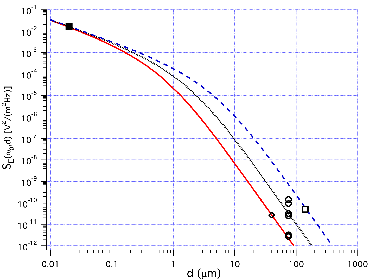
We find that $0.6\zeta_{0}\leq\zeta\leq 4.5\zeta_{0}$ covers the range of ion traps data. As reported in Refs [5, 7], the typical size of static patch potentials on gold surfaces is $\zeta_{0}=1~\mu m$ in excellent agreement with the assumption $\zeta_{0}\gg 20~nm$. We interpret then the residual spread of the experimental data in terms of different correlation lengths (in the range $[0.6,4.5]~\mu m$) associated to the sample surface quality, itself highly dependent on the fabrication technique. The role of surface quality has been noted in ref [13], where successive cleaning procedures decreased the measured electric field noise density (points $\bigcirc$ in Fig. 2). Thus our work shows that in order to compare measured field noise on very different scales, one has to take into account the correlation length of the material and not assume a $d^{-4}$ scaling of the noise, otherwise leading to an over-estimation of the noise at smaller distances. For example, as shown in Fig. 1, our model predicts that for a sample with $\zeta\sim 1~\mu m$, the noise at $d=100~nm$ is $10^{9}$ times greater than noise at $d=100~\mu m$ (at the same frequency), three orders of magnitude lower than expected with a $d^{-4}$ scaling.

In conclusion we developed a model for the electric field noise density based on an analytical approach, assuming a finite size of the potentials patches. Electrical noise field density scaling laws predicted by this model are in very good agreement with experimental results, both in the long range regime (hundred of microns), probed with ion traps experiments and in the short range regime (tens of nanometers) probed with micro-fabricated cantilevers. Let us point out that the pessimistic $d^{-4}$ scaling law for heating rates observed in trapped ion experiments is over estimated in the short range regime. Moreover even though the noise considered in such devices lies within the $MHz$ range, we find a characteristic length compatible with measurement of static potential patches sizes. This opens a new possibility to improve the performances of surface micro-traps based on the analysis of electric static noise obtained with atomic force microscopes.

*

References

- [1] C. I. Sukenik, M. G. Boshier, D. Cho, V. Sandoghdar, and E. A. Hinds, Phys. Rev. Lett. 70, 560 (1993).
- [2] B. C. Stipe, H. J. Mamin, T. D. Stowe, T. W. Kenny, and D. Rugar, Phys. Rev. Lett. 87, 096801 (2001).
- [3] S. Kuehn, R. F. Loring, and J. A. Marohn, Phys. Rev. Lett. 96, 156103 (2006).
- [4] J. M. Lockhart, F. C. Witteborn, and W. M. Fairbank, Phys. Rev. Lett. 38, 1220 (1977).
- [5] J. B. Camp, T. W. Darling, and R. E. Brown, Journal of Applied Physics 69, 7126 (1991).
- [6] F. Rossi and G. I. Opat, Journal of Physics D: Applied Physics 25, 1349 (1992).
- [7] N. Gaillard, M. Gros-Jean, D. Mariolle, F. Bertin, and A. Bsiesy, Applied Physics Letters 89, 154101 (2006).
- [8] R. Blatt and D. Wineland, Nature 453, 1008 (2008).
- [9] D. P. DiVincenzo, Fortschritte der Physik 48, 771 (2000).
- [10] D. J. Wineland, C. Monroe, W. M. Itano, D. Leibfried, B. E. King, and D. M. Meekhof, J. Res. Natl. Inst. Stand. Technol. 103, 259 (1998).
- [11] D. Leibfried, R. Blatt, C. Monroe, and D. Wineland, Rev. Mod. Phys. 75, 281 (2003).
- [12] Q. A. Turchette, D. Kielpinski, B. E. King, D. Leibfried, D. M. Meekhof, C. J. Myatt, M. A. Rowe, C. A. Sackett, C. S. Wood, W. M. Itano, et al., Phys. Rev. A 61, 063418 (2000).
- [13] J. Labaziewicz, Y. Ge, D. R. Leibrandt, S. X. Wang, R. Shewmon, and I. L. Chuang, Phys. Rev. Lett. 101, 180602 (2008a).
- [14] C. Henkel, S. Pötting, and M. Wilkens, Applied Physics B: Lasers and Optics 69, 379 (1999).
- [15] R. Carminati and J.-J. Greffet, Phys. Rev. Lett. 82, 1660 (1999).
- [16] R. J. Epstein, S. Seidelin, D. Leibfried, J. H. Wesenberg, J. J. Bollinger, J. M. Amini, R. B. Blakestad, J. Britton, J. P. Home, W. M. Itano, et al., Phys. Rev. A 76, 033411 (2007).
- [17] C. Henkel and B. Horovitz, Phys. Rev. A 78, 042902 (2008).
- [18] M. G. House, Phys. Rev. A 78, 033402 (2008).
- [19] C.-S. M. R. Paroni, Y. Xiang, and E. A. Kenik, Journal of Computational and Applied Mathematics 190, 200 (2006).
- [20] P. Debye, J. H. R. Anderson, and H. Brumberger, Journal of Applied Physics 28, 679 (1957).
- [21] J. Labaziewicz, Y. Ge, P. Antohi, D. Leibrandt, K. R. Brown, and I. L. Chuang, Phys. Rev. Lett. 100, 013001 (2008b).
- [22] S. Seidelin, J. Chiaverini, R. Reichle, J. J. Bollinger, D. Leibfried, J. Britton, J. H. Wesenberg, R. B. Blakestad, R. J. Epstein, D. B. Hume, et al., Phys. Rev. Lett. 96, 253003 (2006).