A geometric-probabilistic method for counting low-lying states in the Bousso-Polchinski Landscape
Abstract
We propose an accurate method for counting states of close to zero and positive cosmological constant in the Bousso-Polchinski Landscape. This method is based on simple geometrical considerations on the high-dimensional lattice of quantized fluxes and on a probabilistic model (the “random hyperplane” model) which provides a distribution of the values of the cosmological constant. Justification of the assumptions made in this model are offered by means of numerical experiments.
1 Introduction
One of the recent proposals to solve the cosmological constant problem in cosmology is provided by string theory. By dimensional reduction from M-theory to 3+1 dimensions, vacua of the effective theory are classified by means of a big number of quantized fluxes leading to an enormous amount of metastable vacua, the Bousso-Polchinski (BP) Landscape [1]. The cosmological constant problem, namely the smallness of the observed vacuum energy density in the universe [2, 3], can be solved by the presence in this model of a huge number of states of very small, positive cosmological constant, together with a dynamical mechanism given by eternal inflation [4] which allows to visit all the vacua. An anthropic selection is then advocated to explain the smallness of the observed cosmological constant [5, 6].
In order to quantify this selection a counting of accesible states in the Landscape is needed. Two ways of counting have been introduced so far:
- •
The simplest Bousso-Polchinski count, which computes the volume of a spherical shell of small thickness in flux space and divides it by the volume of a cell.
- •
The entropy count of Bousso-Yang, which computes the entropy of the occupation number of each flux assuming that they are independent.
In the following subsection we will briefly review these two counting methods, and drawing on them we will propose an alternative one.
1.1 The Bousso-Polchinski count
The first estimate of this number is given by the BP count. We will now review this argument (see [1]). A vacuum of the BP Landscape is a node in a -dimensional lattice generated by charges determined by the sizes of the three-cycles in the compactification manifold. The lattice is
| (1) |
The -th coordinate of a point in the lattice is an integer multiple of the charge , and therefore a vacuum is characterized by the integer -tuple .
A fundamental cell (also called Voronoi cell11 1 Also called Wigner-Seitz cell in solid state physics, the Voronoi cell of a point in a discrete set of a metric space is the set of points of which are closer to than to any other point of .) around a node in a lattice is the subset of which contains the points which are closer to than to any other node of . Thanks to the discrete translational symmetry of our lattice (1), all fundamental cells in are translates of the fundamental cell around the origin , which we can parametrize in Cartesian coordinates as a product of symmetric intervals
| (2) |
i.e.
| (3) |
The cosmological constant of vacuum in the BP model is22 2 We use reduced Planck units in which .
| (4) |
In (4), is an a priori cosmological constant or order . Each value of defines a spherical ball on the -dimensional flux space of radius . We call this ball . We take small values of the charges (natural values expected by BP are of order ) in such a way that the ball can contain a huge number of fundamental cells.
The number of states in the Weinberg Window, that is the range of values of the cosmological constant allowing the formation of structures (like galaxies) needed for the formation of life as we know it [6], is obtained by computing the volume of a thin spherical shell in flux space (the realization in the BP Landscape of the Weinberg Window) divided by the volume of a cell in the lattice:
| (5) |
where , and the volume of the dimensional sphere is
| (6) |
This method can be naively expected to yield a good estimate when the linear dimensions of the cell are small when compared to the thickness of the shell; but this condition is not satisfied in the BP Landscape. Nevertheless, the result of this counting formula is very good when compared with actual numerical experiments. We will derive the true condition of validity of the BP count in our own framework in section 2 below.
1.2 The Bousso-Yang count
The second estimate is given by the Monte Carlo numerical simulation by Bousso-Yang (BY) in ref. [7]. They compute the number of states by means of the Shannon entropy of the occupation number distribution of each flux in a sample of states obtained in two ways:
- •
Drawing the states from a canonical ensemble distribution with spherical symmetry.
- •
Drawing the states as the output of a decay chain using a dynamical relaxation mechanism.
This method has an advantage: it incorporates the dynamical relaxation mechanism of Brown-Teitelboim (BT) [8, 9], thus quantifying the dynamical selection effect, but two drawbacks should be mentioned:
- •
It makes it necessary to choose particular values for the charges, thereby providing no explicit dependence of the computed number of states with the charges or the dimension, and
- •
They assume that the states of low positive cosmological constant (referred to as penultimate states) have fluxes which are considered independent random variables. A hypothesis which they accept as not true but which they suggest how to correct.
We will briefly review their use of the Shannon entropy for counting.
For any subset having nodes in the Landscape ( can be the set of penultimate states, for example), we can define the uniform probability over as follows:
| (7) |
where is a random variable which can take values over the whole Landscape viewed as a subset of , that is, can be any integer -tuple with equal probability, namely . The Shannon entropy of the uniform distribution satisfies
| (8) |
as can be seen by subtituting (7) into (8) taking . If were not constant over , then it must have support larger than in order to satisfy eq. (8).
If the fluxes were independent, this joint probability would split:
| (9) |
and therefore the correspondent Shannon entropy would be simplified to
| (10) |
Unlike , the distributions are much simpler to estimate by sampling a small portion of . But, as long as they are not constant, its support covers a much larger region than , and furthermore this region has the symmetry of the cell rather than the symmetry of , so we can expect the simplified entropy of eq. (10) to be much larger than the true entropy .
A numerical experiment can be illustrative. Needless to say, the only way to compute the correct uniform probability is to exhaustively compile all the elements of the set , and this is not possible over a realistic Landscape. So we have taken a very simple model of fluxes with and charges , , , and as the set we have considered the secant states (see next subsection). A brute-force count of this set is easily carried out by enumerating all states in it, resulting in or
| (11) |
The same enumeration of all states allows us to compute the three probability distributions , and from these we obtain the additive entropy , and a state count of
| (12) |
which, indeed, means an enormous difference.
It must be stressed that the goal of the BY work is to quantify the dynamical selection effect of the BT decay chain, and they do this by computing the quotient of the number of states with and without dynamics. While both numbers are affected by the independency error, their quotient may be free of errors. We are interested in studying this point in our future research.
1.3 Our counting method
Our proposal is based on the following kinds of states one may encounter near the null cosmological constant surface in flux space:
- •
Boundary (or penultimate after BY) are those states in which a BT decay chain can end before jumping into the negative cosmological constant sea. So we define a boundary state as one having
- (1)
positive cosmological constant, and
- (2)
at least one neighbor of negative cosmological constant.
- (1)
- •
Secant states have the property that their Voronoi cell in flux space has non-empty intersection with the null cosmological constant surface in flux space. Note that a secant state may have negative cosmological constant.
These two categories are not equivalent; a boundary state may not be secant if it is far enough from the null cosmological constant surface, and a secant state may not be boundary if it has negative cosmological constant. So we are interested mainly in the states which are both secant and boundary, because all the states in the Weinberg Window are in this category. Figure 1 illustrates the differences between these two kinds of cell.

Our strategy would be as follows. We will count the states in the Weinberg Window using the following elementary formula:
| (13) |
where
- •
is the number of states in the Weinberg Window,
- •
is the total number of secant states,
- •
the factor is the (first-order) approximate fraction of positive cosmological constant secant states,
- •
is the probability that a random secant state has a positive cosmological constant in the Weinberg Window. If we call a number of the size of , then
(14) where the probability must be computed using the distribution of the cosmological constant as a random variable over all the secant states.
In section 2 we first compute the number and check it with simple models with two or three fluxes, where brute-force counting is feasible. In the following section we propose a probabilistic model (and check it against numerical data) which leads to the distribution of the values of the cosmological constant restricted to the secant states (section 3). We use this distribution to compute the probability (14) in section 4. Surprisingly, our results show that this more precise counting method yields the same result as the BP count. Finally, we summarize the conclusions in section 5.
2 Counting secant states
We start with the observation that the number of secant states which we can find by looking from the origin in a given direction is not a constant, as can be seen in the histogram shown in figure 2.

In this figure, we can also see the theoretical density of states which we now derive for the case.
Let be the number of secant states on the first quadrant of a BP Landscape which are between the 1-axis and a straight line drawn at an angle , as in figure 3.

The number of states along the arc between the 1-axis and the -angle line can be accurately approximated by the length of the segments which the states along the circle are covering. These lengths can be straightened as shown in figure 3, to yield (here we call for convenience)
| (15) |
Its derivative is the directional density of states:
| (16) |
In equation (16), , and . Only the first quadrant is considered here and the absolute value on the components of must be taken if we want to extend equation (16) to all quadrants. The formula thus obtained is plotted in figure 2 over the numerical data, giving an accurately approximated density. Of course we can estimate the total number of secant states by
| (17) |
Using the values , and , we have , being the correct number, obtained by an exhaustive search, of 143 states, 2 of them on the axes, which gives a total of
| (18) |
The two results clearly agree.
For a model with , we can see that the Voronoi cells of the secant states on the first octant project their faces over the first quadrants of planes 1-2, 1-3 and 2-3. The area of these quadrants is and the number of states needed to cover this total area is
| (19) |
Let us now take the density (16) and extend it to . The correct scaling will be
| (20) |
where is a norm-one vector on the sphere. Let us integrate this function on the first octant:
| (21) |
The -integrals have the values 1, 1, , and the -integrals have the values , , , so that all integrals coincide and the result is (19).
Using the values , , , for the model, we have an 8-octant total number of secant states of
| (22) |
A brute-force search of the secant states gives 9205 states on the first octant. But 3 are on the axes, on the coordinate planes and the rest () outside, so the total number of secant states found in this model is
| (23) |
The agreement in this case is not complete but it is satisfactory.
The discrepancy may be caused for the sampling method of the secant states in the brute-force search. It consists on uniformly sampling the sphere of radius correspondent to ; each point thus sampled hits on the intersection between the sphere and the Voronoi cell of certain secant state . Therefore, the probability for this secant state to be selected by this method is proportional to the area (-volume) of the intersection:
| (24) |
If we call the set of secant states , the complete and disjoint partition (tessellation) which the Voronoi cells induce on the sphere guarantees that this probability is normalized:
| (25) |
Thus, only the states with bigger intersection area will be selected in a sample taken by this method. In addition, the intersection volume is positive but it does not have a positive lower bound, so in principle there can be arbitrarily small intersections which will not be detected by this method. In the case, points were needed to find the existing 143 secant states (see figure 1), but using points on the case yielded 9134 states of the 9205 revealed in the sample. If the set contains states with a probability below , these will not be found using this method. So the agreement may increase by taking a sample size greater than .
Let us extend the directional density of states (20) to an arbitrary dimension and to all “quadrants”:
| (26) |
where , and . The number of secant states is
| (27) |
The integration measure on the sphere is invariant under rotations, and there is a rotation which can transform a given coordinate in the simplest of them, , in the following choice of coordinates for the sphere:
| (28) |
where is the last vector in a basis. The integration measure reduces to
| (29) |
so that
| (30) |
We have then
| (31) |
In a somewhat nonstandard way, we have defined the quantity
| (32) |
Equations (22) and (17) are special cases of (31). A more explicit form of (31), using and is
| (33) |
Let us now derive the condition of validity of formulae (31, 33). Note that we are summing the number of times that a fundamental cell fits in a -quadrant; in order for this number to represent the actual number of secant states, the excess -volume of the cells trying to fit the boundary must be very small when compared with the -volume of the -quadrant. The -volume of the cell projection is different in each direction, so we can compute a kind of mean value of the projection volume as
| (34) |
where and are respectively the geometric and harmonic means of the charges. This mean projection volume must be much less than the -volume of a single -quadrant, that is,
| (35) |
After substituting and , we find33 3 Incidentally, this relation resembles the so-called t’Hooft limit in field theory, in which the number characterizing the gauge group tends to infinity and the Yang-Mills coupling constant vanishes with the product (the t’Hooft coupling) held fixed.
| (36) |
3 The random hyperplane model
We assume two basic features of the secant states in a BP Landscape:
- •
The Voronoi cells of the secant states are small enough to replace the sphere which intersects the cell by its tangent hyperplane.
- •
The orientations of the hyperplane intersecting the cell are random if one picks a secant state at random.
In this way, we propose to study the set of secant states by choosing a probability measure on the secant hyperplane set. In this section we first parametrize the hyperplane space, and then we choose a probability measure on it.
3.1 The hyperplane space
We define as the set of all hyperplanes in and as the set of all hyperplanes with non-empty intersection with :
| (37) |
In order to specify a hyperplane we must choose, first of all, a normal vector of unit norm, . A point in must also be given; but there is an infinity of possible choices here, and we must provide a unique prescription, for example the point closest to the origin (chosen here as the center of ). Note that this point may lie inside or outside .
The pair has a lot of redundant information, because the directions of the vector and coincide, that is, . Therefore, we must retain only the norm of and the whole ; letting , we can identify with the pair . Also, we must take into account the fact that and represent different hyperplanes if , but the same hyperplane if , so the vector is defined up to a sign in the case .
An alternative equivalent prescription is to consider directions up to a sign for all (the point is on with antipodal points identified, i.e. a point on the projective space ). In this case, represents not only the minimum distance from the hyperplane to the origin , but also the position of the hyperplane “above” or “below” the origin. We find the former point of view more adequate.
The domain of definition of is a direction-dependent positive interval , and is determined by the restriction that the hyperplane it represents has non-empty intersection with . In particular, the point of minimum distance can lie outside ; thus, the “hyperplane space”, when compared with “physical” space, comprises a larger region than .
We now compute , defined as the maximum distance to the origin of the closest point to the origin of a hyperplane with non-empty intersection with the cell . Clearly, the corners of the cell are the most far away points in , so for each direction , the last (most distant) hyperplane orthogonal to and with non-empty intersection with must contain one of the corners of the cell. The equation of such a hyperplane is
| (38) |
where is the unique corner out of which belongs to the same -quadrant as , and the are signs , indeed the same signs of the components of , that is, . This hyperplane is already in normal form, so its minimum distance to the origin is
| (39) |
Given a direction , the closest point can be found as the intersection of the line with the hyperplane (38). This method is used to construct the hyperplane space for the case in figure 4, where it is compared with formula (39).

The function can be plotted for and , , versus a polar angle defined as , see figure 5.

3.2 A probability measure in the hyperplane space
Now we need to define a probability measure on the hyperplane space just parametrized. The simplest choice is the uniform probability on :
| (40) |
where is the characteristic function on , whose effect is simply to restrict the integration domain to , and is the volume measure in . is a normalization constant:
| (41) |
We can compute by first integrating out the variable in (41):
| (42) |
By comparing equations (26) and (39) we observe the following relation between the maximum distance of a hyperplane in a given direction and the directional density of states :
| (43) |
so that using the definition of the density of states
| (44) |
we have
| (45) |
In the last formula we have substituted the expression for found in equation (31).
The main reason for choosing the uniform probability measure is its simplicity. The physical reason is that among all measures in a given compact space, the uniform one has maximum Shannon entropy. In the following, we will justify our choice by more quantitative means.
First of all, the marginal probability in the variable associated to the uniform measure is proportional to the directional density of states , with a normalization-to-one factor:
| (46) |
Therefore, the uniform probability reproduces the correct directional density of states as observed in the numerical experiments.
On the other hand, we can plot instances of the set of secant hyperplanes and compare them with simulated uniform points in hyperplane space. The simplest of such plots is for ; with and charges , , we show the points from the actual secant hyperplanes versus a simulated set of uniform points of equal sample size in figure 6.


The geometrical nature of the secant hyperplane sample is revealed in the structures shown in fig. 6 (left), which introduces correlations in the spatial sequence. In contrast, a uniform sample in hyperplane space (fig. 6, right) shows no correlations, and the only structures which we can see are voids and clusters bigger than the ones present in the former case.
Both samples thus obtained (the secant hyperplane set, or geometric sample, and the uniformly distributed points, or simulated sample) cover the hyperplane space, so we can approximate the distribution of the former set of points by a uniform probability, thus neglecting the spatial correlations.
But the efficiency of the covering is not equal in both cases: the geometrical sample shows smaller voids and clusters than the simulated one. This can be seen by counting the number of points inside a circle of random position and given radius inside the hyperplane space in both cases (fig. 7 illustrates this “circle method”).
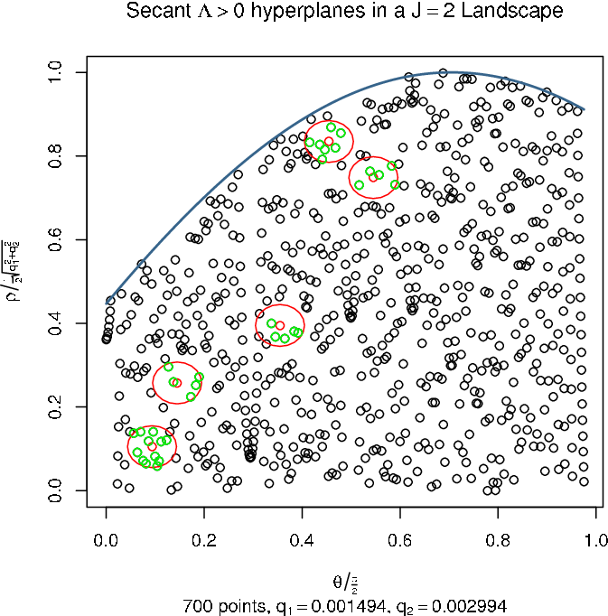
When this is done for a big number of such circles, the voids and clusters induce a fluctuation in the number of “inner” points, which will be greater if the inhomogeneities are bigger.


Fig. 8 shows the result presented as two histograms of the number of inner points for circles. These can be well approximated by Gaussians, and we can see that the variance of the simulated sample is bigger than the variance of the geometric one: that is, the geometric points cover hyperplane space with a more regular (less random) pattern, in such a way that each point tries to avoid the clusters and tends to fill the gaps, a characteristic behavior of the so-called quasi Monte Carlo (qMC) sequences [11].
Putting the comparison in more a quantitative fashion, the mean and standard deviation of the geometric and simulated samples are
| (47) |
The different mean values with the same number of points indicate that the density of points is not the same in both samples. This happens because the spatial correlations in the geometric case make the left and right sides underpopulated (see fig. 6), so that the effective volume covered in this case is smaller. We can take this into account by considering the quotient between the standard deviation and the mean as a measure of the clustering of the data, which is an effective scaling of the data to have mean value 1. This leads to
| (48) |
This means that the fluctuation in the point density is greater for the simulated sample. The relative difference is considerable (, that is, 31%). This indicates that the covering of the hyperplane space by the geometric sample is much more efficient than the covering made by the simulated one, and thus its randomness is much smaller.
Summarizing, the approximation made by assuming uniformity in the distribution of secant hyperplanes is equivalent to neglecting the spatial correlations present in the geometric case, and we can expect this approximation to work well because of the more efficient covering of hyperplane space in this case.
4 Number of states in the Weinberg Window
The next step in our calculation is to compute the distribution of values of the cosmological constant. The random hyperplane model allows us to do this by means of the marginal probability distribution in the variable, whose density will be called :
| (49) |
Using the following relation between (the minimum distance from a tangent hyperplane to their secant state), (the radius of the sphere) and the Euclidean norm of the secant state in flux space (which in turn is related to the cosmological constant)
| (50) |
the distribution can be found once the function is computed:
| (51) |
The function is easily computed once the integration of the characteristic function in the variables is reversed. The variable takes a maximum value , and the variable can range across . So we define the integral of an arbitrary test function on the hyperplane space against the probability measure as
| (52) |
For the iterated integrals, we have the following identity44 4 In equation (53), we drop the constant computed in (45). (Fubini’s theorem):
| (53) |
where the sets and appear owing to , and are defined as
| (54) |
Note that the restrictions in both sets are the same, , but in the direction remains fixed, and in the distance remains fixed. So, is simply the interval used in the integral (46), and is a set which is the whole sphere when and a -connected-component set when . If we carry out the integration of but we stop before the integration, we have
| (55) |
To compute the integral in (55) in closed form is not an easy task, and even if it were, it would be useless, because the function is built by gluing polynomial functions in a -dependent number of intervals.
Let us compute for the simplest case. The set is here an interval, which can be computed from the function which represents the upper boundary of hyperplane space, see fig. 5. A horizontal line at height has two, one or no intersection with in the first quadrant depending on . Taking , there are no intersection points if , there is a single intersection point if and there are two intersection points if . The equation to be solved for the intersection points in the first quadrant is (remember that in we have )
| (56) |
Setting , we have a quadratic equation whose solution has two branches:
| (57) |
These branches only make sense for (for ) and for (for ). We define , so we have, in the first quadrant only,
| (58) |
The function is, then,
| (59) |
With , , and taking and charges , , we can plot this function and compare it with the true histogram of the secant states; this is done in figure 9 (left), where we see big fluctuations of the number of states versus the theoretical function.


This strong fluctuation is a consequence of the relative sparsity of this Landscape. The small sample size makes the histogram oscillate around the theoretical curve; we believe that this effect is only present in , as can be seen in the subsequent figures.
In figure 9 (right) we can see the relative error between the exact formula (59) and the Monte Carlo evaluation explained below (eq. (61)). They agree in the constant region, and the error remains smaller than for all values.
We can compute the values of the function numerically by rewriting it in the following way, using the unit step function for restricting the integrand to and the formula (45) for the normalization constant :
| (60) |
Thus, the formula splits in a constant times the mean value of the step function with respect to the uniform probability measure on the sphere. This mean value is easily computed using a simple Monte Carlo technique, that is, sampling the unit sphere with a large number of points , we have
| (61) |
The Monte Carlo evaluation is well suited for this task, because the integrand is bounded and the integration domain is compact.
In fig. 10 we can see the MC-computed distribution for Landscapes with and , where brute-force data are available. The oscillates much more than the one, due in part to the bin width, which contributes to make the histogram smoother with a bigger sample size. But the mean value in the constant region (as well as the global fit to the entire theoretical curve) seems to be better adjusted in the case. The reason for this apparent disagreement between the brute-force data in and the theoretical MC-computed curve is the sampling method used to find the secant states in this case. This sampling method, described above (see section 2), has the disadvantage of missing the states with very small area of the intersection polytope between the sphere and the Voronoi cell of the secant state. Using eq. (31), we can estimate the number of missing states; with , , , , , we have
| (62) |
The brute force calculation yielded 406,715 states in the first 4-quadrant; taking into account degeneracies (the degeneracy of each state is , being the number of zero-flux components), we obtain
| (63) |
Their difference relative to the mean degeneracy is
| (64) |
These states amount to 5.4% of the total, and they lie completely in the high- region. This is the reason why the theoretical curve disagrees with the histogram in the case: the histogram is normalized to have total area one and it misses 5% of states of higher , so we must conclude that the data range of the histogram must be shorter and its constant region must be higher, as shown in fig. 10.


But we don’t need the numerical evaluation to analyze the function. From eq. (59) we can see that when , the value of the step function is always 1, so we have the exact result
| (65) |
that is, the distribution of values is exactly constant at small , . Beyond this value, the step function finds regions where , and the mean value begins to decrease monotonically. When , no point in the sphere is captured by the step function, and vanishes. We have checked this general behavior on high-dimensional BP models before and after performing the BT decay chain and this qualitative profile is quite robust [12].
As the authors of [13] point out, actual histograms of on particular BP Landscapes show a “staggered” behavior which gets smoothed when the bin width increases, but the mean value of these oscillations is given by . Note that is really a discrete variable, and is the density of a continuous one. Furthermore, note that in [13] the authors compile statistics on entire Landscape instances, while our statistics refer to the positive secant state sector only.
So we find that behaves as a Fermi-like distribution on the values, with a medium filling level and a decreasing interval which depend on the values of the charges. Further quantitative analysis must be done trough the numerical estimation procedure described above.
Now, we can compute the probability for the cosmological constant to lie in the Weinberg Window, using the properties of and formula (51):
| (66) |
After inserting this in formula (13), together with eq. (31), we have
| (67) |
This result exactly coincides with the BP count (eq. (5)).
One may wonder if the approximations made by the random hyperplane model are too crude to achieve a better result than the BP count, or if the BP count is a better result than expected. In order to clarify this point, we have again performed a numerical experiment to compare the number of states predicted by the BP (and our) count with a brute-force search of states in a shell of variable width (that is, varying ) in a Landscape with 2,333 secant states in the first octant. In our opinion, the nature of the example chosen would render the approximations made too crude, but we find a remarkable agreement, as shown in fig. 11, and in a range of shell widths much wider than expected.

We are forced to conclude that the BP count has proved to be a succesful way of counting states in the BP Landscape, in fact better than expected. The geometric interpretation is curious; if we sum up the volume of the Voronoi cells of the secant states whose center are inside a shell of prescribed width, we obtain the volume of the shell with very good approximation. In figure 12 we illustrate the spatial location of the states inside the shell for chosen shell widths in the Landscape of the previous example. These locations are uncorrelated for low values of the shell width.


5 Conclusions and future directions
We have modeled the BP Landscape by means of the random hyperplane model (RHM), validated by several numerical experiments like brute-force search and precise state counting. The RHM provides us with a distribution of values of the cosmological constant and reproduces the BP count in a very different way. The numerical experiments performed suggest that the BP count is much more precise than expected, far better than the BY count, for example, and applicable to a wide range of parameters of the Landscape.
Further corrections to this formula can take into account the asymmetry of the and states due to the curvature of the sphere (neglected here), which is a second order effect which depends on the precise values for the charges. For us, it is certainly more difficult to take into account the spatial correlations, which would require a completely different approach.
All these considerations lie in the context of finding an a priori distribution of the cosmological constant, without any reference to the dynamics of the BT decay chain. In our future research we will try to incorporate the dynamical effects as well, in order to count also the states selected by dynamics and to quantify the dynamical selection effect within this framework. In this respect, we have checked by extensive numerical simulations that the Fermi-like profile of the ditribution on the secant states persists even on a subset selected by the BT decay chain [12]. If this effect reveal a feature of the dynamical selection or is caused by the geometric structure of the set of secant states is a point which is worth of further investigation.
Appendix A Improving the BP count
We can slightly improve the result obtained using eq. (13) and the random hyperplane model (RHM) described above. The first heuristic approach is to replace the factor in (13) by a measure of the volume of a shell above and below the surface in flux space. This surface is a sphere of radius . We will call the inside region of this sphere and its volume . We can draw a shell of width above the sphere and another shell of the same width below. Then, the relative volume of the positive- region in the shell is given by the quotient of the volume of the upper shell and the total volume of the two shells:
| (68) |
In the limit or , which is eq. (13), and for the special case (when the inner shell completely fills ) , which is arbitrarily close to 1 for high enough . So we are replacing the by a quantity , and therefore the improvement is small.
It remains to determine what the relevant width is. To this end we use the RHM: the distribution has a Fermi-like profile, and thus we can define a kind of “Fermi level” as the width of a step function distribution that has the same height as and is also normalized to one, that is, . Thus can play the role of the effective width of the secant state set.
Another approach which also takes into account the difference in the volumes of the inner and outer shells is to modify the probability measure in hyperplane space (40) and so the RHM itself. Note that the variable is the distance between the tangent hyperplane and the secant state, so that is the radial spherical coordinate in flux space of the point in the hyperplane closest to the secant state. Therefore the natural modification in the probability measure (40) would be
| (69) |
In this alternative viewpoint of the RHM the variable can be positive or negative, but the weights of the two possibilities are different because the marginal distribution in the variable is not symmetric:
| (70) |
where is the same function as before extended to negative values of by symmetry . Now, we change eq. (13) by
| (71) |
because the new probability distribution carries the difference between the positive and negative states.
As long as , this modification will be harmless and the new probability will be exactly the old one, recovering (13). But if takes on high values, then the asymmetry will be enormous: the distribution (70) will develop a sharp peak in the positive region, far away from the Weinberg Window.
To see how this phenomenon can happen, we can remember that is bounded by its maximum value , which behaves as , being the square root of the second moment of the charges. The extreme case can be written as
| (72) |
But then we are leaving the condition of validity (36), where we have replaced by .
Note that unfamiliar things happen when conditions like (36) are violated. We can see this by choosing a fixed small typical charge and increasing the dimension . The distance from the corner of the cell and its center, , can thus reach the radius , that is, the Voronoi cell around the origin in flux space will eventually find its corners touching the surface of the sphere55 5 The cell acquires a kind of “dendritic” structure, with its faces lying far away from the sphere and its corners touching it. An enormous fraction of the volume of such a small, -dimensional cell is located at its corners. of radius . At this point all states inside the sphere will be secant; of course many states outside the sphere will be secant also, and a huge fraction of them will be in the corners of a parallelotope enclosing the sphere. But the vast majority of these states will not have neighbors of negative cosmological constant, and therefore the typical value of in these states will be large, hence the peak in the distribution mentioned above.
We see that once the validity condition is violated, the majority of the secant states are no more boundary states, and thus the secant states in this regime have no special relation with the Weinberg Window. But the secant state set is simply a tool to study the boundary state set , which comprises the states selected by dynamics, and we can use instead of only when they significantly overlap. We believe that this is the case when the validity conditions are satisfied.
Acknowledgments
We would like to thank Roberto Emparan for useful discussions. We also thank Concha Orna for carefully reading this manuscript. This work has been supported by CICYT (grant FPA-2006-02315) and DGIID-DGA (grant 2007-E24/2). We thank also the support by grant A9335/07 (Física de alta energía: Partículas, cuerdas y cosmología).
References
- [1] R. Bousso and J. Polchinski: Quantization of four-form fluxes and dynamical neutralization of the cosmological constant. JHEP 06, 006 (2000) [hep-th/0004134].
- [2] S. Weinberg: The cosmological constant problem. Rev. Mod. Phys. 61, 1-23 (1989).
- [3] R. Bousso: TASI Lectures on the Cosmological Constant. Gen. Rel. Grav. 40 (2008) 607 [0708.4231 [hep-th]].
- [4] A. H. Guth: Inflation and Eternal Inflation. Phys. Rept. 333 (2000) 555 and references therein [astro-ph/0002156].
- [5] L. Susskind: The Anthropic Landscape of String Theory. [hep-th/0302219].
- [6] S. Weinberg: Anthropic Bound on the Cosmological Constant. Phys. Rev. Lett. 59, 2607-2610 (1987).
- [7] R. Bousso and I. Yang: Landscape predictions from cosmological vacuum selection. Phys. Rev. D 75 (2007) 123520 [hep-th/0703206].
- [8] J. D. Brown and C. Teitelboim: Dynamical neutralization of the cosmological constant. Phys. Lett. B195, 177 (1987).
- [9] J. D. Brown and C. Teitelboim: Neutralization of the cosmological constant by membrane creation. Nucl. Phys. B297, 787-836 (1988).
- [10] R Development Core Team: R: A language and environment for statistical computing. R Foundation for Statistical Computing, Vienna, Austria. ISBN 3-900051-07-0 (2007), http://www.R-project.org.
- [11] See, e.g., sec. 8.3 in R. Crandall and C. Pomerance: Prime Numbers: A Computational Perspective. Springer-Verlag New York (2001).
- [12] C. Asensio and A. Segui, in preparation.
- [13] D. Schwartz-Perlov and A. Vilenkin: Probabilities in the Bousso-Polchinski multiverse. JCAP 0606, 010 (2006), hep-th/0601162.