Metastable supersymmetry breaking
and multitrace deformations of SQCD
Abstract
Metastable vacua in supersymmetric QCD in the presence of single and multitrace deformations of the superpotential are explored, with the aim of obtaining an acceptable phenomenology. The metastable vacua appear at one loop, have a broken R-symmetry, and a magnetic gauge group that is completely Higgsed. With only a single trace deformation, the adjoint fermions from the meson superfield are approximately massless at one loop, even though they are massive at tree level and R-symmetry is broken. Consequently, if charged under the standard model, they are unacceptably light. A multitrace quadratic deformation generates fermion masses proportional to the deformation parameter. Phenomenologically viable models of direct gauge mediation can then be obtained, and some of their features are discussed.
1 Introduction
Relaxing the requirement that supersymmetry breaking occurs in the true vacuum (see e.g. [1]–[3]) can help overcome many of the constraints of dynamical supersymmetry breaking with no supersymmetric vacua [4]. Recently, Intriligator, Seiberg and Shih [5] have shown that metastable dynamical supersymmetry breaking is rather generic and easy to achieve. They found that metastable vacua occur in supersymmetric QCD (SQCD), in the free magnetic range, when the quarks have small masses,
| (1.1) |
This has opened many new avenues for model building and gauge mediation; see [6]–[22] for some examples of recent work, and [23] for a review and a more complete list of references.
It is not possible to build a phenomenologically viable model of gauge mediation using directly the ISS superpotential (1.1). This is due to an unbroken R-symmetry that forbids non-zero gaugino masses. A natural question is then how the phenomenology changes when the superpotential is a more general polynomial in . While this has been considered before for some particular superpotential deformations (see e.g. [11, 14, 16, 20, 21]), a more detailed account of the space of metastable vacua and the low energy phenomenology is needed. For instance, the light fermions of the model have not been fully explored. The aim of this work is to analyze the IR properties of the theory and its phenomenology in the presence of a generic -preserving polynomial superpotential
| (1.2) |
where is some large UV scale, is an order one coefficient, and ‘’ are sextic and higher dimensional operators.
Deforming (1.1) by a generic polynomial in breaks R-symmetry explicitly at tree level, and additional supersymmetric vacua are introduced [24]. The supersymmetric vacua for a single trace superpotential were analyzed in detail in [16], where it was found that the magnetic theory has classical supersymmetric vacua with various possible unbroken subgroups of the magnetic gauge group. This should be contrasted with the case of ISS, Eq. (1.1), where the magnetic gauge group is completely Higgsed and supersymmetry is broken classically by the rank condition.
After taking into account one loop quantum corrections in the magnetic theory, one finds the deformed theory also has metastable vacua at low energies [16]. The dynamical reason for this is that the deformations to the magnetic superpotential come from irrelevant operators in the electric theory, which are parametrically suppressed. Therefore, we end up with a controllable deformation of the ISS construction in the IR. These vacua break R-symmetry spontaneously, and in phenomenologically interesting regions of parameter space the spontaneous breaking is much larger than the explicit breaking.
Since supersymmetric vacua allow for unbroken magnetic gauge groups, one might expect the same to occur for metastable vacua. However, the metastable vacua in the theories we explore below have a completely broken magnetic gauge group; vacua with unbroken subgroups of the magnetic gauge group do not occur. This is in some disagreement with [16] and it would be interesting to see how this effect appears in the brane constructions of metastable vacua [25].
Next we will analyze the phenomenological properties of the spectrum, with particular attention to the light fermions, including the Standard Model gauginos and a multiplet of fermions from the “meson” superfield . If the superpotential contains only single traces of powers of , the singlet and adjoint parts of the meson superfield have the same one loop effective action. The singlet fermion is the Goldstino, and must be massless at one loop through a cancellation of its nonzero tree level mass against a one loop correction. The adjoint fermions (or more precisely, a certain subset thereof) have the same tree and one loop effective action, and so their masses arise only at two loops (and/or through equally small mixing effects.) Consequently their masses are small compared with those of the Standard Model gauginos, which arise at one loop.
In this paper we will be considering the case where the embedding of the Standard Model gauge group into the flavor group endows these fermions with Standard Model quantum numbers. With such light masses, these fermions would already have been observed, and so these models would be phenomenologically unacceptable.
We are therefore led to consider a multitrace deformation of the superpotential; in particular, we must take in Eq. (1.2). Then the cancellation between the tree level and one loop masses for the Goldstino fails for the adjoint fermions, leaving them with masses proportional to . The phenomenology of direct gauge-mediated models based on this theory is quite rich, since the adjoint fermions may be lighter or heavier than the Standard Model gauginos, depending on . Mixing between these fermions and the gauginos is negligibly tiny, due to a charge-conjugation symmetry in (1.2). We will briefly discuss some of the interesting phenomenological properties of such a scenario, leaving the details to a forthcoming publication [26].
The various sections are arranged as follows. In Section 2, we discuss the moduli space of SQCD with the superpotential Eq. (1.2), keeping only terms up to quartic order in the electric fields. In Section 3, we review SQCD without deformations (ISS), with emphasis on the spectrum and associated phenomenological issues. In Section 4, we study single trace deformations of the ISS superpotential, that is, the case . We show that all metastable vacua have a magnetic gauge group that is completely Higgsed, and we discuss the spectrum, showing it is unacceptable for phenomenology. Next, in Section 5 we consider , describing the spectrum in detail. Finally, Section 6 contains a brief overview of the phenomenology of and constraints on such models. Various computations are shown in detail in the Appendix.
2 SQCD with a multitrace superpotential
In this section, we analyze the symmetries and supersymmetric vacua of SQCD in the presence of a generic -preserving polynomial superpotential.
Supersymmetric QCD with gauge group and flavors with equal masses has a global symmetry group
| (2.1) |
under which transform as . There is also a discrete charge conjugation symmetry . For phenomenological applications we will later weakly gauge a subgroup of and identify it with the Standard Model gauge groups. We will also gauge to remove a Nambu-Goldstone boson.
The most general quartic superpotential preserving this symmetry is of the form
| (2.2) |
We will typically consider , and take to be of order one or smaller. We will not consider sextic or higher operators, since they are suppressed by higher powers of and would not affect our discussion. The nonrenormalizable superpotential (2.2) could be generated from a renormalizable theory, for example by integrating out fields with masses that couple to .
Let us consider the theory in various limits. First, for there is a moduli space of vacua parameterized by mesons and baryons modulo classical constraints. The global symmetry is enhanced to , and there is a non-anomalous symmetry as well as an anomalous axial current.
For but , the superpotential is renormalizable, and the theory has an exact classical symmetry which is anomalous at the quantum level.11 1 There is also an approximate non-anomalous R-symmetry “” which is restored as , but we will not need to consider this symmetry. The non-anomalous symmetries of the model are
plus the charge conjugation. The F-term relations lift the moduli space and the only vacuum is at the origin.
On the other hand, for and large but finite, all R-symmetries are explicitly broken at the classical level. New discrete supersymmetric vacua appear in the regime
2.1 Magnetic dual
Below the scale , the theory is described by an effective theory, called the “dual magnetic theory”, with gauge group , singlet mesons , and fundamental flavors ; we define . The theory has a positive beta function and is weakly-coupled in the infrared. After an appropriate change of variables, the classical tree level superpotential reads
| (2.3) |
where the first trace is over magnetic color and the remaining traces are over flavor indices. The relation with the electric variables is (roughly)
More details may be found in [5].
As in ISS, we restrict to small quark masses . We will also restrict ourselves to the range
| (2.4) |
which guarantees that . This will be needed to have long-lived metastable vacua. There are nonperturbative corrections to the superpotential (2.3), but they are all small enough not to affect our calculations given (2.4).
Also, these conditions ensure that the symmetries of the model at the scale are approximately , broken to only by effects of order and . Therefore, to an excellent approximation, both the superpotential and the Kähler potential satisfy the larger symmetry group, under which the trace and traceless parts of transform as a single irreducible multiplet. We will work only to leading non-vanishing order in the symmetry-breaking effects from non-zero and non-infinite .
Furthermore, the discrete charge-conjugation symmetry of the electric theory appears as the transformation
| (2.5) |
This transformation plays an important role in the phenomenology of gauge mediation models based on (2.3), and indeed in other ISS-related models (see e.g. [32]).
As in the electric theory, the R-symmetry is explicitly broken, and we expect new supersymmetric vacua parametrically at . Indeed, the solutions to the F-term constraints
| (2.6) |
are
| (2.7) |
and
| (2.8) |
with . (Here represents the identity matrix, and a subscript indicates a block matrix of the corresponding size.) The appearance of the extra parameter classifying different classical vacua has been observed for by [16]. In particular, for there is an unbroken magnetic gauge group .
3 Metastable DSB in the R-symmetric limit
In the next three sections, we will analyze the IR dynamics of (2.3) in three steps. First, we review the ISS model [5], the R-symmetric limit , which corresponds to an electric SQCD with massive flavors and no irrelevant operators. We will highlight the spectrum and associated phenomenological problems. In Section 4, we show how these problems are not entirely solved by making non-zero but leaving . Finally, in Section 5, we show how the theory with resolves the remaining problems.
3.1 The model and its spectrum
The ISS model considers massive SQCD near the origin in field space in the free magnetic range , where the theory has a dual magnetic description with superpotential
| (3.1) |
At the classical level the theory breaks supersymmetry by the rank condition. We parametrize the fields by
| (3.2) |
| (3.3) |
where is the rank of the magnetic gauge group. The classical moduli space of vacua is parametrized by and . The other fields have vanishing expectation values. In the rest of the paper we will restrict to metastable vacua with maximal unbroken global symmetry, by choosing the ansatz
| (3.4) |
It will be checked that this is a self-consistent choice.
The vev for breaks the gauge group completely, with the breaking pattern
| (3.5) |
(Here all groups except are global; we remind the reader that ). The reduction of the global symmetry group leads to Nambu-Goldstone modes. The fields are charged under , which plays the role of a messenger number symmetry. See [5] for a more detailed discussion.
The flat directions are not protected by holomorphy or symmetries and, as we shall review shortly, become massive at one loop. (A field with these properties is called a “pseudo-modulus” [5].) In particular, is stablized at the origin. Near the origin of moduli space the rank condition imposes
| (3.6) |
and the scale of supersymmetry breaking is
| (3.7) |
To analyze the spectrum of the theory, it is convenient to rewrite the superpotential in terms of the component fields,
| (3.8) | |||||
The spectrum consists of three sectors, each consisting of fields satisfying .
(1) The sector: Treating as a background superfield, the supersymmetric mass matrix is
| (3.9) |
while the bosonic matrix is computed, as usual, including off-diagonal blocks with F-terms.
There are Dirac fermions that come from and . Near the origin of field space, their masses are of order , from (3.9). The scalars combine into complex fields, which are linear combinations of . There are complex Nambu-Goldstone bosons from the combinations and . The remaining complex scalars have splittings of order, and centered around, . The numerical coefficients adjust to preserve .
This sector will play the role of the messenger sector in gauge mediation applications. Once a subgroup of the flavor symmetry is identified with the Standard Model, and gauged with couplings , the Nambu-Goldstone modes will acquire a one loop mass of order . (In particular, we will study the case where is gauged — see Eq.(3.5).) The lightest state will be stable in the full theory, since the messenger sector is protected by the non-anomalous messenger number.
(2) The sector: Fermions from form Dirac fermions with mass . The traceless part22 2 We denote traceless fields with primes; for instance is the traceless part of . of the chiral superfield , which contains the NG bosons , is eaten by the superHiggs mechanism when the magnetic group is gauged.
The field is a NG boson associated to the breaking of . The field corresponds to a pseudo-modulus, which will be lifted at one loop. The fermion from is massless. This sector has a supersymmetric spectrum at tree level.
The massless fields from would be phenomenologically forbidden. This forces us to gauge , so that the superfield is eaten by the gauge boson and at tree level acquires a mass of order .
(3) The sector: is a flat direction, with massless fermionic partner at tree level. In particular, is the Goldstino.
One loop contributions from heavy particles lift the pseudo-moduli. The fields do not couple at tree level to the supersymmetry breaking sector, so they do not contribute to the one loop effective potential for the pseudo-moduli. Because we are in the regime where is of order the square of the messenger masses, the effect of integrating out the messengers does not have a simple expression in superspace, and it is more convenient to work directly with nonsupersymmetric expressions. The bosonic action is given by the usual Coleman-Weinberg formula [27]
| (3.10) |
Near the origin of moduli space , the potential is approximated by [5]
| (3.11) |
with
| (3.12) |
Therefore, in the ISS model the pseudo-moduli are consistently stabilized at the origin and R-symmetry is preserved. In this approximation, the one loop mass of the bosonic field is given by
| (3.13) |
3.2 Phenomenological problems
One could try to use the ISS construction as the supersymmetry breaking sector in models of direct gauge mediation. However, since R-symmetry is preserved in the metastable vacuum, Majorana masses for the Standard Model gauginos are forbidden. The same applies to the fermions and , which may have SM quantum numbers after embedding the SM gauge group into the flavor symmetry group of the model. For these reasons, this model does not give an acceptable phenomenology.
There are various ways of improving this situation (see, for instance, [28]–[31]). One very interesting proposal [32] is that the gauginos could come from Dirac fermions, whose mass is not constrained to vanish by an unbroken R-symmetry. This idea was applied to the ISS model in [33], by adding new fields and interactions to the superpotential. Dirac masses appear from one loop diagrams mixing the MSSM Weyl gauginos with the new Weyl fermions. One problem with this approach is that doubling the number of fields (in order to have Dirac fermions) creates a Landau pole close to the messenger scale. In this case, corrections from the microscopic theory may become important.
4 Single trace deformation
We begin by considering the superpotential Eq. (2.3) with , that is, with only a single trace perturbation:
| (4.1) |
This model was discussed in [16], where it was suggested that new metastable vacua, with unbroken magnetic group, appear around . However, this region of parameter space is subtle, because higher order corrections to (3.11) become important. We will have two new things to say about this model.
(1) By considering the full logarithmic one loop potential (3.10), it is possible to show that the metastable vacua with unbroken magnetic gauge group are actually unstable. Thus, one is led to study only the ISS-like vacuum where the magnetic gauge group is completely Higgsed.
(2) Gauginos indeed become massive at one loop in this model, as expected from the R-symmetry breaking. However (ignoring some subtleties which we will discuss later) the adjoint fermions become massive only at two loops, because diagrammatic cancellations that make the Goldstino massless at one loop also force the adjoint fermions to be massless at this order. This provides the main motivation for studying non-zero below.
4.1 Metastable supersymmetry breaking
The classical supersymmetric vacua are obtained by setting in (2.7) and (2.8). In order to analyze the effect of the deformation on the ISS metastable vacuum, the cases and have to be distinguished.
Case
This is the analog of the ISS construction, with no unbroken gauge group. The fields are parameterized as in Eqs. (3.2) and (3.3). We will now review why a metastable vacuum appears at a distance of order away from the origin [16].
As a starting point, set . Due to the classical deformation, is no longer a flat direction, unlike the ISS case. Rather, the origin is at the side of a paraboloid of classical curvature . In other words, the origin is unstable against classical flow of toward the supersymmetric vacua discussed before. The tree level spectrum near the origin is shown in Figure 1.

In order to create a local minimum, the quantum contribution should overwhelm the curvature of the classical potential, i.e., . This rather interesting effect, where a one loop contribution stabilizes a classical runaway direction, was analyzed in [15]. Here, the stabilization of can occur naturally, since , arising from a nonrenormalizable operator in the microscopic theory, is parametrically small. The condition that the one loop potential introduces a supersymmetry breaking minimum,
| (4.2) |
is naturally satisfied.
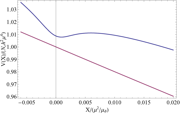
The potentials at tree level and at one loop, as a function of , are shown in Figure 2. As seen from the figure, the tree level potential (lower magenta curve), which is obtained from the superpotential in (4.1), has no supersymmetry breaking minimum. A metastable minimum is created near the origin once the one loop quantum corrections in the form of are included (upper blue curve).
As a result of the competition between the classical and quantum contributions, a metastable vacuum is created at
| (4.3) |
see Eq. (3.4) for the notation. As expected, is proportional to the explicit R-symmetry breaking parameter . However, it is larger than this by the inverse loop factor . This follows from the fact that the minimum appears from balancing a tree level linear term of order against a one loop quadratic term of order .
The pattern of symmetry breaking in this vacuum is
| (4.4) |
where only the messengers transform under . Unlike the ISS construction, here , so that the R-symmetry is both explicitly and spontaneously broken, with the latter dominating since .
Case
The possibility of metastable vacua with is very interesting; coupling this to the MSSM, it would imply unbroken gauge groups in the hidden sector. Properties of such configurations were discussed in [16]. Unfortunately, we will now show that there are generically no metastable vacua in this regime.
Such vacua should be of the form
| (4.5) |
The parametrization of the fluctuations is slightly more involved,
| (4.6) |
and similarly for . As in the case , the expectation values are chosen to be of the form
The new fields and do not exist for . They are fundamental flavors of the unbroken magnetic group .
As was found in [16], positivity of the bosonic mass matrix of implies
This places us in the regime . In this regime, the quadratic approximation (3.11) to the Coleman-Weinberg potential is no longer valid. For , all the higher order terms in give contributions comparable to (3.11). In other words, it is necessary to use the full expression appearing in Eq. (3.10).
Therefore, to establish the existence of such vacua, a detailed analysis of is required. As shown in the Appendix, all such vacua are unstable once the full form of is included. The intuitive reason for this is that at large the logarithmic growth of cannot overwhelm the quadratic terms in the classical potential. A similar behavior was found in [15].
The plot of for this case is almost the same as that of Figure 2. For sufficiently large , the classical falling potential dominates the logarithmic rise of the , and no critical points are found until the supersymmetric vacuum is reached.
Summarizing, metastable states occur only for . The fields have expectation values Eq. (4.3), breaking the magnetic gauge group completely at the scale .
4.2 Light fermions
We therefore return to the one remaining vacuum, the ISS-like case with . From the previous analysis, the bosons from and the traceless part of acquire masses of order . The aim of this section is to compute the fermion masses at one loop, and show that remains massless at this order, contrary to naive expectations from R-symmetry breaking.
First we explore one loop effects involving the Goldstino . At tree level it has a nonvanishing mass . We are not expanding around a critical point of the classical potential, but rather one of the full one loop potential, and therefore the Goldstino should become massless only once one loop effects are included. This implies that the one loop diagram has to give
| (4.7) |
such that . Indeed, the explicit evaluation of the one loop diagram in the Appendix corroborates (4.7). These results are approximate because we are neglecting (subleading) mixings with other singlet fermions; see below and the Appendix.
At a first glance it is surprising that the one loop contribution can be equal to the tree level one. This is so because the one loop diagram is of order
However, since , with defined in Eq. (3.12), we obtain the result (4.7). This is another manifestation of the pseudo-runaway behavior discussed in the previous section.
Next, notice that within the classical superpotential (4.1), only appears in single traces. On the other hand, the one loop contribution is a single trace of a function of , because it comes from exponentiating bosonic and fermionic determinants (denoted by ) arising from messengers in the fundamental representation of . Therefore, the full one loop effective action
can be written as a single trace of products of and its superpartner. This means that the tree level plus one loop contribution to the masses of the fields must be of the form , and therefore the singlet and adjoint parts of get identical masses through one loop. The same is true for the fermionic partners of : at one loop the masses of the singlet and the adjoint are the same. Diagrammatically, there is a cancellation between the tree level Weyl mass and the one loop correction.
We note two small subtleties. First, we have assumed here that the kinetic terms for the singlet and adjoint parts of have the same normalization. This is true to a very good approximation. We assumed , which ensured that the high-energy theory’s approximate symmetry is only weakly broken to at the scale . Under this larger symmetry, the singlet and adjoint transform as a single irreducible representation, assuring equally normalized kinetic terms, up to negligible order() corrections.
Second, and irreducibly, the Goldstino is not quite . As discussed in more detail in the Appendix, it mixes slightly with the fields and , with mixing angles of order a one loop factor, and , respectively. Consequently the tree level and one loop masses fail to cancel precisely, though by an amount that is one further loop-order suppressed. Thus our statement that the masses vanish at one loop is effectively correct.
4.3 Phenomenology of the model
After gauging a subgroup of the flavor group — see Eq. (3.5) — and identifying it with the Standard Model gauge group, the adjoint fermions will carry Standard Model gauge charges. The fact that they are approximately massless at one loop is unacceptable phenomenologically. They do become massive at two loop order, through the above-mentioned mixings, and through explicit two loop diagrams. For example, Standard Model gauge bosons, which do not impact the singlet , generate for the other fields a two loop mass of order
| (4.8) |
But the Standard Model gauginos have a one loop mass of order . Importantly, the charge conjugation symmetry discussed in Section 2 forbids significant mixing between and , so the masses for the fields cannot be raised through mixing effects. Consequently, requiring the gauginos are at a scale 1 TeV implies the would be so light that they would have already been observed.
5 The deformation with
Clearly the root of this phenomenological problem lies in treating and the Goldstino on the same footing in the tree level superpotential. A solution is to allow non-zero ,
| (5.1) |
such that the two have different tree level masses. Then the total one loop mass for becomes proportional to .
The motivation for considering non-zero
| (5.2) |
extends beyond phenomenological utility. No symmetry enforces once or even are non-zero, so it is quite natural for to be nonzero.33 3 Considering the preserved symmetries, one might wonder why the coefficients of should be taken precisely equal. The point is that the physical couplings are constrained by the approximate in the electric theory, which is still valid at and just below the scale . In other words, the and limit implies equal couplings. Nothing comparable favors .
Let us now analyze the metastable vacua of the theory. For (and for roughly of order 1), the Coleman-Weinberg potential is approximately as in ISS. The only stable local minimum occurs for . The multitrace deformation adds a term proportional to the identity matrix to , so we obtain
| (5.3) |
| (5.4) |
with
In the limit , the effect of is qualitatively unimportant:
| (5.5) |
so that . While does not alter the qualitative features of the vacuum, it is important, when computing the spectrum, that the precise values (5.3) and (5.4) be used.
5.1 Spectrum
We now analyze the spectrum in the metastable vacuum. As in Section 4, the Goldstino is not massless at tree level. Some of the one loop diagrams exactly cancel the tree level contributions and for this reason we discuss directly the tree level plus one loop results.
We first consider the fermions of the pseudo-modulus . The singlet fermion (the Goldstino) is massless at one loop. For the adjoint fermions, the tree level mass is partially canceled against the one loop contribution, and the full mass is of order
| (5.6) |
Of course this vanishes in the limit , as required from Section 4.
Interestingly, we will see in Section 6 that the Majorana gaugino masses are proportional to . By changing the dimensionless parameter , the adjoint fermions may thus be made lighter or heavier than the gauginos. This allows a variety of spectra with different phenomenological signatures, see Section 6.
As for the bosons of , both the adjoint and one component of the singlet acquire one loop masses of order ; see Eq. (3.13). The other part of the singlet, Arg(), is a massive R-axion. This is because has a large nonzero expectation value , which spontaneously breaks the approximate symmetry at a scale much larger than any explicit breaking. The mass of the R-axion is given by
| (5.7) |
This is of the same order as the one loop mass , Eq. (3.13).
Finally, the and sectors are as in Section 3.1. We remind the reader that we have gauged the symmetry, and denotes its gauge coupling. The (otherwise massless) fields from acquire masses of order , as shown in the table. Furthermore, the NG bosons from acquire a one loop mass of order once the Standard Model is gauged, as a subgroup of the flavor symmetry group. The lightest of these is stable due to the unbroken messenger number from Eq. (4.4).

5.2 Lifetime of the metastable vacuum
Here we check that the metastable non-supersymmetric vacuum can be sufficiently long-lived. This vacuum can decay to the ISS-like supersymmetric vacuum with , or to the supersymmetric vacua with (see Section 2.1). The decay to the vacua with requires changing the expectation value of (some of the elements of) , from to . This is strongly suppressed by the quartic potential term . The dominant decay channel will be to the supersymmetric vacuum with , which we now analyze.
The lifetime of the vacuum may be estimated using semiclassical techniques and is proportional to the exponential of the bounce action, [34]. We will see that the tunneling takes place in the direction of , in a region where is almost constant. The potential as a function of , including the one loop quantum corrections from the Coleman-Weinberg potential, is given in the Appendix and shown in Figure 2. It may be modeled as a triangular barrier, and the bounce action may be estimated using the results in [35].
We will see in the next section that, in order to have large enough gaugino masses but a low SUSY-breaking scale and low sfermion masses, the ratio cannot be made too small. Nonetheless, it is useful to first analyze the bounce action in the limit , where it is clear the vacuum is parametrically stable.
The dimensionful parameters controlling the shape of the potential are and . We assume , , , and are all of order 1. The SUSY vacua are parametrically far away from the metastable vacua in the limit
| (5.8) |
In this limit, the calculation of the bounce action is very similar to that done in [15], as long as only varies. Let us assume is essentially constant.
The metastable SUSY-breaking vacuum lies at , the peak of the potential is near , and the SUSY vacuum is at , where phases and numbers have been ignored. Moreover, the potential difference between the peak and the metastable SUSY-breaking minimum is roughly , much smaller than . The results of [35] then show that the field tunnels not to the SUSY vacuum directly but rather to . For this value of , Eq. (2.6) implies , and thus indeed stays approximately constant in the tunneling region. This confirms that the results in [35] apply.
In the limit , the bounce action scales parametrically as
| (5.9) |
where we have neglected some numerical factors, see [35]. Thus, as , and the metastable vacuum can be made parametrically long-lived.
In Section 6, we will see that in order to obtain sfermion masses that are roughly of the same size as gaugino masses, we need to take (and thus .) In this regime , and are all parametrically of order . A numerical study is required to determine the existence and lifetime of the metastable vacuum. Taking the gaugino masses to lie at their experimental lower bound, of order 100 GeV, we find that the existence of a metastable vacuum sets a lower bound on the sfermion masses — typically a few TeV for the squarks and at least a few hundred GeV for the right-handed sleptons. Once such a metastable vacuum is obtained, it is easy to make the bounce action larger than the required 400 by a small increase (of order 5%) in the sfermion masses. The details of the spectrum, together with a more precise estimate of the lower bound on the sfermion masses, and the implications for the tuning of electroweak symmetry breaking, will be given in [26].
6 Comments on the phenomenology
This section briefly discusses some of the phenomenology associated with the multitrace deformation of the ISS model, equation (5.1). The details will be left to a forthcoming publication [26].
The ISS-like supersymmetry breaking models are interesting from a phenomenological point of view due to the presence of the large global symmetry group
| (6.1) |
A model of direct gauge mediation can be built by weakly gauging a subgroup of (6.1) and identifying it with the Standard Model (SM) gauge group. The fields , , , and in (3.2) and (3.3) act as messengers that mediate the supersymmetry breaking effects to the visible sector. Loops involving these messengers can give non-zero masses to the scalar superpartners of the SM fermions and, provided there is no unbroken R-symmetry, non-zero Majorana fermion masses to the gauginos.
In this section, we will consider gauging the subgroup of for in the model, and identifying it with the SM gauge group. (The effect of gauging a subgroup of will be discussed in [26].)
Under the SM gauge group , the adjoint field decomposes as
| (6.2) |
The fermions from the superfields , , and carry the same gauge charges as the gluino, wino, and bino, respectively, and the first two could be directly produced at colliders.44 4 The bosons in (6.2) get a mass of order (10 TeV) from the Coleman-Weinberg potential and are thus rather heavy. If produced in the early Universe, they would have decayed promptly into and a gaugino, excepting gauge singlets which would decay a bit more slowly through higher dimension operators. Also, there are new light fermions from the superfields and ; these are stable unless given new interactions, and require a special discussion below.
6.1 Phenomenology of and
A very important property of the model is that the gauginos and the adjoint do not mix. This is due to the fact that and have charge conjugation transformations that differ by a sign,
| (6.3) |
This discrete symmetry forbids any mixing at low orders between the two sets of fermions. More precisely, -violation in the SM allows and to mix, but this occurs only at three loops and is thus negligibly small.
Let us estimate the gaugino and masses. As discussed in Section 5.1, the metastable vacuum has an approximate R-symmetry that is spontaneously broken through the non-zero vev , where is a loop factor (3.12). Therefore, gauginos obtain a one loop mass of order
| (6.4) |
Neglecting numbers and factors of the gauge coupling , an interesting phenomenology is obtained for
| (6.5) |
i.e. for
| (6.6) |
The also obtain a mass at one loop, which, using equation (5.6), is of order
| (6.7) |
neglecting factors of and and other numbers. By adjusting , can be made heavier or lighter than , leading to very different collider signatures as we will discuss next.
The do not mix with the Standard Model gauginos at a level that determines their decays. Instead, if they are heavy enough, they can decay (promptly) into a gaugino and a gauge boson through the dimension five operator :
| (6.8) |
The gauginos can decay through all the usual supersymmetric decay modes, and/or through the standard coupling of each gaugino to a gauge boson and Goldstino:
| (6.9) |
If instead the are lighter than the gauginos, then the gauginos will decay into the plus a gauge boson via the above-mentioned operator. The decays to a gauge boson and an off-shell gaugino. The precise decay modes and the lifetime of the depend on the details of the spectrum, and will be discussed further in [26].
From (6.2), we see that there are new fermions, with charges and . By binding to quarks, these form hadrons, some of which are charged. The lightest of these novel hadrons, whether charged or neutral, would be stable in the model as described so far. But this would be ruled out, since these hadrons would have been created in the early Universe, violating the bounds on the existence of heavy stable particles [36, 37]. These fermions must thus be made to decay through additional baryon-number violating operators in the superpotential and/or the Kähler potential. In [26], we will show that additional dimension five Kähler potential terms, coupling the adjoint to SM quarks and leptons, can allow the fermions to decay without affecting Big-Bang Nucleosynthesis or violating current bounds on proton decay.
6.2 Sfermion masses, the SUSY-breaking scale and a light gravitino
Since the supersymmetry breaking scale is and the mass scale of the messengers is of the same order, the soft scalar masses are roughly given by
| (6.10) |
Comparing this to (6.4), the sfermions and gauginos have similar masses if
| (6.11) |
We recall that the existence and longevity of the metastable vacuum requires , see Section 5.2.
More concretely, there is an interesting parameter region characterized by (6.11) and a low supersymmetry breaking scale
| (6.12) |
In this case, one can show (see [26]) that the heaviest sfermions (squarks) have masses of a few TeV, the lightest sfermions (right-handed sleptons) haves masses of a few hundred GeV, the gaugino masses are of order several hundred GeV, and there is a large enough lifetime for the metastable vacuum. The gravitino mass is
| (6.13) |
where GeV is the reduced Planck mass. Such a light gravitino does not violate any cosmological or astrophysical constraints [43].
6.3 Further comments on the spectrum
As discussed in Section 5, the messenger sector contains real NG bosons, all of which become massive at one loop after weakly gauging the flavor symmetry. In the parameter range (6.12), this mass is of order of several TeV. The messenger number in (4.4) forbids the decay of the lightest of these messenger particles, which is thus stable. If the lightest messenger is neutral and weakly interacting and has an appreciable relic density, it would have a tree-level coupling to nuclei via -boson exchange and would have been seen at a dark matter direct detection experiment [38]-[42]. If the stable state is charged and/or colored, the experimental constraints are even stronger [36, 37]. Thus experimental constraints rule out the possibility that the lightest messenger is dark matter; this will be investigated further in [26].
We also note that the SM gauge couplings have a Landau pole well below the GUT scale, due to the presence of extra matter charged under the SM gauge group. As one runs up to the high scale, the gauge coupling blows up first at about GeV for , so that new physics has to enter at or below this scale. Larger values of lower this scale to the point that it affects our discussion materially. See [44] for a recent discussion of the Landau pole problem in ISS-like SUSY-breaking models.
6.4 Illustrative choices of parameters
We postpone a careful study of the various constraints to [26], but preliminarily it appears possible to satisfy simultaneously all of the conditions considered above. For example, for ,55 5 In this case, the magnetic gauge group is trivial and, after a field redefinition, the superpotential is given by (2.3) plus . For this term is negligible near the origin, so our analysis is self-consistent. the parameters of the electric theory Eq. (2.2) that are consistent with (6.11) and (6.12) are of order 0.01–10 TeV, TeV, and TeV. With these choices, the models appear to have no insuperable problem below the scale of the Landau pole.
On the other hand, for , has to be below TeV, and the ratio is not parametrically small. In this case, the corrections from the microscopic theory are not guaranteed to be small, and the violations of the approximate symmetries may be large. In particular, the cancellations described in section 4.2 may be imperfect, requiring a more elaborate analysis. However, the argument for nonzero still holds, and its effects can still dominate, in which case the phenomenology outlined here will be largely unchanged.
6.5 Summary
While these models are not yet entirely plausible, they represent an advance over the models with gauged and , which as we showed are excluded by the presence of overly-light charged and colored fermions. We have demonstrated that with , it is possible to obtain models with a long-lived metastable vacuum, a spectrum with all standard model superpartners in the TeV range, and with no obvious unresolvable conflict with any experiment.
The minimal versions of these models have new TeV-scale fermions in the adjoint representations of the Standard Model gauge group that do not mix with standard model gauginos. They also have squarks and sleptons significantly heavier than the gauginos, and exotic stable hadrons which must be made to decay through additional interactions. They also suffer from the ubiquitous intermediate-scale Landau pole for standard model gauge couplings. We will pursue various associated model-building issues, and study in more detail the phenomenology of these models in [26].
Acknowledgments
We would like to thank Evgeny Andriyash, Masahiro Ibe, Paul Langacker, David Shih, and especially Scott Thomas for valuable discussions. This research was supported by DOE grant DE-FG01-06ED06-02. R.E. is supported by the US DOE under contract number DE-AC02-76SF00515. K.S. is supported by NSF grant PHY-0505757 and the University of Texas A&M. G.T. would like to thank KITP for their hospitality and support through the NSF Grant PHY05-51164.
Appendix A One loop calculations
In this appendix we collect the one loop calculations for the ISS model with multitrace quadratic deformations. The superpotential is
| (A.1) |
where , and .
A.1 Messenger sector
Let us consider separately the cases and (see Section 4.1).
Case
The parametrization of the metastable minima is given by Eqs. (3.2) and (3.3). Around these minima the superpotential is
| (A.2) | |||||
and the non-zero F-term is
| (A.3) |
We recall the ansatz (3.4),
| (A.4) |
The vev completely Higgses the dual gauge group and the . To determine , one must compute the Coleman-Weinberg potential from the tree level masses of the messenger sector. The ansatz (A.4), which will be checked self-consistently, simplifies the computations since the mass eigenstates are then independent of their flavor index. One can thus suppress color and flavor indices in the following.
The messenger sector contains the fields , , and , that couple to the non-zero F-term. Let us define
| (A.5) |
for the messenger gauge eigenstates. The Weyl fermions combine into Dirac fermions and the messenger masses can be written as
| (A.6) |
where the messenger mass matrices are
| (A.7) |
and
| (A.8) |
For the fermionic and bosonic messenger masses are ( and )
| (A.9) | |||||
| (A.10) | |||||
The fermion masses have multiplicity while the complex boson masses have multiplicity .
The messenger mass matrices can be diagonalized by unitary matrices , and such that
| (A.11) |
where , and are messenger mass eigenstates. The quadratic lagrangian for the messengers is therefore of the canonical form
| (A.12) |
Due to the charge conjugation symmetry, it is possible to write the mixing matrices such that and . This can be easily seen from the mass matrices for . This property will be useful when computing one loop corrections to light masses.
Case
The fluctuations are parametrized as in Eq. (4.6), so there are extra messenger superfields . The analysis of proceeds along the same lines as in the case , except that the fermion messenger masses have now multiplicity while the complex boson messenger masses have multiplicity .
The masses of and are ()
| (A.13) |
The fermion masses have multiplicity while the complex boson masses have multiplicity . Importantly, in the limit of small deformation, (A.13) forces to avoid tachyons.
A.2 One loop bosonic action
The tree level pseudo-moduli are given by and , and they are stabilized by one loop contributions. For , the one loop effective potential for is the same as in [5] (see Eq. (3.11).) As a result, this field is stabilized at the origin and acquires a mass of order .
Let us now analyze the pseudo-modulus ; for , this is a matrix. The ISS-type vacua correspond to . We will argue here that the new metastable vacua corresponding to the case do not exist, as they are located in a region where some of the fields become tachyonic. The only remaining metastable vacua will be the ISS-type vacua.
The one loop correction from integrating out the messenger fields is
| (A.14) | |||||
with masses given in Section A.1. We find that the full potential
| (A.15) |
has a metastable vacuum if , but there are no metastable vacua for . Let us discuss in more detail how this occurs.
For , the messengers are non-tachyonic for any ; see Eq. (A.9). As explained in Section 4.1, the metastable vacuum appears because quantum corrections at small are large enough to overwhelm the slope of the classical potential, which would otherwise push toward the supersymmetric vacua. The supersymmetry breaking vacuum is located in the range , far from the supersymmetric vacuum.
The situation for is very different, because the messengers are tachyonic at small ; see Eq. (A.13). For these tachyons are absent, but in this regime the one loop corrections grow only logarithmically with , and cannot compete with the classical potential to create a metastable vacuum. One may directly check that the Hessian of the potential always has a negative eigenvalue for (and all values of ). Notice that if one used the quadratic expansion of around the origin , instead of the full logarithmic form, it would suggest the existence of metastable vacua with and [16]. But this approximation is inconsistent, and when the full logarithmic dependence of is included, these vacua become unstable and disappear.
Summarizing, only the ISS-type minima with survive, and the adjoint () and singlet () components of the pseudo-modulus acquire one loop masses
| (A.16) | |||||
| (A.17) |
The R-axion, discussed in section 5.1, has a mass of this same order, Eq. (5.7). All bosons which were light at tree level thus become heavy at one loop, with masses of order .
A.3 One loop fermionic action
In this section we discuss the low energy fermionic spectrum of the theory, taking into account one loop effects.
Goldstino
At one loop, the Goldstino appears as a combination of , and , which we now determine. The charge conjugation symmetry forbids mixings with , which is eaten by the gauge fermion and has mass .
First, at tree level, in the limit , and form a Dirac fermion of mass , while is massless; see Eq. (A.2). When and are nonzero, acquires a mass term proportional to , and there is a - mixing of order . There is no linear combination of the fields , and that is massless at tree level.
Once one loop effects are taken into account, supersymmetry is spontaneously broken, so we should get a massless Goldstino. Since the dominant F-term comes from , the Goldstino will be approximately aligned with . Indeed, the tree level plus one loop mass element is (using the messenger mass eigenbasis),
| (A.18) |
where the sums are over messenger fields and
| (A.19) |
It can be checked that the tree and one loop terms in (A.18) largely cancel, leaving only a term of order , of the same size as two loop corrections.
There are also one loop mixings between and , . For simplicity, let us consider first the ISS model, corresponding to the limit . The mass-mixing comes from the two-point function , which is allowed by R-symmetry. A calculation along the same lines as in (A.18) shows that this mass-mixing is of order . The Goldstino is hence predominantly in the direction, with a small (of order ) component along . This implies that in ISS, one loop corrections generate a nonzero F-term
For nonzero but small, the Goldstino also has a small component along , with mixing angle of order . This is smaller than the mixing of and , and is consistent with a one loop F-term
Gauginos and the fermions
There are no mixings between the gauginos and the fermions at one and two loops, because they are forbidden by charge conjugation. The expression for the one loop gaugino mass is
| (A.20) |
which is of order . The one loop computation for the masses of is nearly identical to that of , given in (A.18), since they have the same interactions with the messenger fields. The result is
| (A.21) |
The cancellation that occurs in (A.18) occurs here as well, but leaves over a large remainder, of order .
References
- [1] H. Murayama, “A model of direct gauge mediation,” Phys. Rev. Lett. 79, 18 (1997) [arXiv:hep-ph/9705271]. S. Dimopoulos, G. R. Dvali, R. Rattazzi and G. F. Giudice, “Dynamical soft terms with unbroken supersymmetry,” Nucl. Phys. B 510, 12 (1998) [arXiv:hep-ph/9705307].
- [2] M. A. Luty, “Simple gauge-mediated models with local minima,” Phys. Lett. B 414, 71 (1997) [arXiv:hep-ph/9706554]. M. A. Luty and J. Terning, “Improved single sector supersymmetry breaking,” Phys. Rev. D 62, 075006 (2000) [arXiv:hep-ph/9812290].
- [3] T. Banks, “Cosmological supersymmetry breaking and the power of the pentagon: A model of low energy particle physics,” arXiv:hep-ph/0510159.
- [4] S. D. Thomas, “Recent developments in dynamical supersymmetry breaking,” arXiv:hep-th/9801007.
- [5] K. Intriligator, N. Seiberg and D. Shih, “Dynamical SUSY breaking in meta-stable vacua,” JHEP 0604, 021 (2006) [arXiv:hep-th/0602239].
- [6] T. Banks, “Remodeling the pentagon after the events of 2/23/06,” arXiv:hep-ph/0606313.
- [7] A. Amariti, L. Girardello and A. Mariotti, “Non-supersymmetric meta-stable vacua in SU(N) SQCD with adjoint matter,” JHEP 0612, 058 (2006) [arXiv:hep-th/0608063].
- [8] M. Dine, J. L. Feng and E. Silverstein, “Retrofitting O’Raifeartaigh models with dynamical scales,” Phys. Rev. D 74, 095012 (2006) [arXiv:hep-th/0608159].
- [9] H. Abe, T. Higaki, T. Kobayashi and Y. Omura, “Moduli stabilization, F-term uplifting and soft supersymmetry breaking terms,” Phys. Rev. D 75, 025019 (2007) [arXiv:hep-th/0611024].
- [10] M. Dine and J. Mason, “Gauge mediation in metastable vacua,” Phys. Rev. D 77, 016005 (2008) [arXiv:hep-ph/0611312].
- [11] R. Kitano, H. Ooguri and Y. Ookouchi, “Direct mediation of meta-stable supersymmetry breaking,” Phys. Rev. D 75, 045022 (2007) [arXiv:hep-ph/0612139].
- [12] H. Murayama and Y. Nomura, Phys. Rev. Lett. 98, 151803 (2007) [arXiv:hep-ph/0612186].
- [13] H. Murayama and Y. Nomura, Phys. Rev. D 75, 095011 (2007) [arXiv:hep-ph/0701231].
- [14] C. Csaki, Y. Shirman and J. Terning, “A simple model of low-scale direct gauge mediation,” JHEP 0705, 099 (2007) [arXiv:hep-ph/0612241].
- [15] R. Essig, K. Sinha and G. Torroba, “Meta-Stable Dynamical Supersymmetry Breaking Near Points of Enhanced Symmetry,” JHEP 0709, 032 (2007) [arXiv:0707.0007 [hep-th]].
- [16] A. Giveon and D. Kutasov, “Stable and Metastable Vacua in SQCD,” Nucl. Phys. B 796, 25 (2008) [arXiv:0710.0894 [hep-th]].
- [17] B. K. Zur, L. Mazzucato and Y. Oz, “Direct Mediation and a Visible Metastable Supersymmetry Breaking Sector,” arXiv:0807.4543 [hep-ph].
- [18] F. q. Xu and J. M. Yang, “An Extension for Direct Gauge Mediation of Metastable Supersymmetry Breaking,” arXiv:0712.4111 [hep-ph].
- [19] N. Haba and N. Maru, “A Simple Model of Direct Gauge Mediation of Metastable Supersymmetry Breaking,” Phys. Rev. D 76, 115019 (2007) [arXiv:0709.2945 [hep-ph]].
- [20] A. Giveon, A. Katz and Z. Komargodski, “On SQCD with massive and massless flavors,” JHEP 0806, 003 (2008) [arXiv:0804.1805 [hep-th]].
- [21] A. Giveon, A. Katz, Z. Komargodski and D. Shih, “Dynamical SUSY and R-symmetry breaking in SQCD with massive and massless flavors,” JHEP 0810, 092 (2008) [arXiv:0808.2901 [hep-th]].
- [22] K. Intriligator, D. Shih and M. Sudano, “Surveying Pseudomoduli: the Good, the Bad and the Incalculable,” arXiv:0809.3981 [hep-th].
- [23] K. A. Intriligator and N. Seiberg, “Lectures on Supersymmetry Breaking,” Class. Quant. Grav. 24, S741 (2007) [arXiv:hep-ph/0702069].
- [24] A. E. Nelson and N. Seiberg, “R symmetry breaking versus supersymmetry breaking,” Nucl. Phys. B 416, 46 (1994) [arXiv:hep-ph/9309299].
- [25] A. Giveon and D. Kutasov, “Gauge symmetry and supersymmetry breaking from intersecting branes,” Nucl. Phys. B 778, 129 (2007) [arXiv:hep-th/0703135].
- [26] R. Essig, J.-F. Fortin, K. Sinha, M. Strassler, G. Torroba, to appear.
- [27] S. R. Coleman and E. Weinberg, “Radiative Corrections As The Origin Of Spontaneous Symmetry Breaking,” Phys. Rev. D 7, 1888 (1973).
- [28] S. Abel, C. Durnford, J. Jaeckel and V. V. Khoze, “Dynamical breaking of U(1)R and supersymmetry in a metastable vacuum,” Phys. Lett. B 661, 201 (2008) [arXiv:0707.2958 [hep-ph]].
- [29] H. Abe, T. Kobayashi and Y. Omura, “R-symmetry, supersymmetry breaking and metastable vacua in global and local supersymmetric theories,” JHEP 0711, 044 (2007) [arXiv:0708.3148 [hep-th]].
- [30] F. Brummer, “A natural renormalizable model of metastable SUSY breaking,” JHEP 0707, 043 (2007) [arXiv:0705.2153 [hep-ph]].
- [31] D. Marques and F. A. Schaposnik, “Explicit R-Symmetry Breaking and Metastable Vacua,” arXiv:0809.4618 [hep-th].
- [32] P. J. Fox, A. E. Nelson and N. Weiner, “Dirac gaugino masses and supersoft supersymmetry breaking,” JHEP 0208, 035 (2002) [arXiv:hep-ph/0206096]. G. D. Kribs, E. Poppitz and N. Weiner, “Flavor in Supersymmetry with an Extended R-symmetry,” arXiv:0712.2039 [hep-ph].
- [33] S. D. L. Amigo, A. E. Blechman, P. J. Fox and E. Poppitz, “R-symmetric gauge mediation,” arXiv:0809.1112 [hep-ph].
- [34] S. R. Coleman, “The Fate Of The False Vacuum. 1. Semiclassical Theory,” Phys. Rev. D 15, 2929 (1977) [Erratum-ibid. D 16, 1248 (1977)].
- [35] M. J. Duncan and L. G. Jensen, “Exact tunneling solutions in scalar field theory,” Phys. Lett. B 291, 109 (1992).
- [36] P. F. Smith, J. R. J. Bennett, G. J. Homer, J. D. Lewin, H. E. Walford and W. A. Smith, “A Search For Anomalous Hydrogen In Enriched D-2 O, Using A Time-Of-Flight Spectrometer,” Nucl. Phys. B 206, 333 (1982).
- [37] M. L. Perl, P. C. Kim, V. Halyo, E. R. Lee, I. T. Lee, D. Loomba and K. S. Lackner, “The search for stable, massive, elementary particles,” Int. J. Mod. Phys. A 16, 2137 (2001) [arXiv:hep-ex/0102033].
- [38] S. Dimopoulos, G. F. Giudice and A. Pomarol, “Dark matter in theories of gauge-mediated supersymmetry breaking,” Phys. Lett. B 389, 37 (1996) [arXiv:hep-ph/9607225].
- [39] M. W. Goodman and E. Witten, “Detectability of certain dark-matter candidates,” Phys. Rev. D 31, 3059 (1985).
- [40] R. Essig, “Direct Detection of Non-Chiral Dark Matter,” Phys. Rev. D 78, 015004 (2008) [arXiv:0710.1668 [hep-ph]].
- [41] J. Yoo [CDMS Collaboration], “Results from the CDMS 5-Tower Operation,” arXiv:0810.3527 [hep-ex].
- [42] J. Angle et al. [XENON Collaboration], “First Results from the XENON10 Dark Matter Experiment at the Gran Sasso National Laboratory,” Phys. Rev. Lett. 100, 021303 (2008) [arXiv:0706.0039 [astro-ph]].
- [43] M. Viel, J. Lesgourgues, M. G. Haehnelt, S. Matarrese and A. Riotto, “Constraining warm dark matter candidates including sterile neutrinos and light gravitinos with WMAP and the Lyman-alpha forest,” Phys. Rev. D 71, 063534 (2005) [arXiv:astro-ph/0501562].
- [44] S. Abel and V. V. Khoze, “Direct Mediation, Duality and Unification,” arXiv:0809.5262 [hep-ph].