Three-Dimensional Simulations of Dynamics of Accretion Flows Irradiated by a Quasar
Abstract
We study the axisymmetric and non-axisymmetric, time-dependent hydrodynamics of gas that is under the influence of the gravity of a super massive black hole (SMBH) and the radiation force produced by a radiatively efficient flow accreting onto the SMBH. We have considered two cases: (1) the formation of an outflow from the accretion of the ambient gas without rotation and (2) that with weak rotation. The main goals of this study are: (1) to examine if there is a significant difference between the models with identical initial and boundary conditions but in different dimensionality (2-D and 3-D), and (2) to understand the gas dynamics in AGN. Our 3-D simulations of a non-rotating gas show small yet noticeable non-axisymmetric small-scale features inside the outflow. The outflow as a whole and the inflow do not seem to suffer from any large-scale instability. In the rotating case, the non-axisymmetric features are very prominent, especially in the outflow which consists of many cold dense clouds entrained in a smoother hot flow. The 3-D outflow is non-axisymmetric due to the shear and thermal instabilities. In both 2-D and 3-D simulations, gas rotation increases the outflow thermal energy flux, but reduces the outflow mass and kinetic energy fluxes. Rotation also leads to time variability and fragmentation of the outflow in the radial and latitudinal directions. The collimation of the outflow is reduced in the models with gas rotation. The time variability in the mass and energy fluxes is reduced in the 3-D case because of the outflow fragmentation in the azimuthal direction. The virial mass estimated from the kinematics of the dense cold clouds found in our 3-D simulations of rotating gas underestimates the actual mass used in the simulations by about 40 %. The opening angles () of the bi-conic outflows found in the models with rotating gas are very similar to that of the nearby Seyfert galaxy NGC 4151 (). The radial velocities of the dense cold clouds from the simulations are compared with the observed gas kinematics of the narrow line region of NGC 4151.
Subject headings
accretion, accretion – disks – galaxies: jets – galaxies: kinematics and dynamics– methods: numerical – hydrodynamicsI. Introduction
Active Galactic Nuclei (AGNs) are powered by accretion of matter onto a super massive (–) black hole (SMBH), and produce a large amount of energy (e.g., Lynden-Bell 55) as electromagnetic radiation (–), over a wide range of wavelengths (from radio to hard X-rays, and even to TeV photons). The strong radiation from AGNs influences the physical properties (e.g., the ionization structure, gas dynamics and density distribution) of their vicinity, their host galaxies, and even of the inter-galactic material of galaxy clusters to which they belong (e.g., Quilis, Bower, & Balogh 85; Dalla Vecchia et al. 21; McNamara et al. 60; Zanni et al. 100; Fabian et al. 29; Vernaleo & Reynolds 94). The importance of the radiation-driven outflows from AGNs as a feedback process is recognized in many of the galaxy formation/evolutionary models (e.g., Ciotti & Ostriker 13, 2001, 2007; King 41; Hopkins et al. 35; Murray, Quataert, & Thompson 64; Sazonov et al. 88; Springel, Di Matteo, & Hernquist 90; Brighenti & Mathews 11; Fontanot et al. 31; Wang, Chen, & Hu 97, Tremonti, Moustakas, & Diamond-Stanic 93; Ciotti et al. 2008, in preparation).
The formation of AGN outflows, of course, can be caused by some mechanisms other than radiation pressure, e.g., magnetocentrifugal force (e.g., Blandford & Payne 7; Emmering, Blandford, & Shlosman 26; Königl & Kartje 45; Bottorff et al. 10), Poynting flux/magnetic towers (e.g., Lovelace et al. 54; Lynden-Bell 56, Lynden-Bell 57; Li et al. 52; Kato et al. 40; Nakamura et al. 65; Kato 39), and thermal pressure (e.g., Weymann et al. 98; Begelman, de Kool, & Sikora 5; Everett & Murray 28). However, the highly blueshifted line absorption features often seen in the observed UV and optical spectra of AGNs can be best described by the radiation-driven wind models (e.g., Murray et al. 63; Proga et al. 84; Proga & Kallman 82), provided that the ionization state of the gas is appropriate. In reality, these forces may interplay and contribute to the dynamics of the outflows in AGNs in somewhat different degrees (e.g., Königl 44; Proga 79, and references therein).
The AGN environment on relatively large scales ( pc) is a mixture of gas and dust (e.g. Antonucci 1; Miller & Goodrich 61; Awaki et al. 3; Blanco et al. 6; Krolik 48). The radiation pressure on dust can drive the dust outflows, and their dynamics is likely to be coupled with the gas dynamics (e.g., Phinney 75; Pier & Krolik 76; Emmering et al. 26; Laor & Draine 51; Königl & Kartje 45; Murray et al. 64). On much smaller scales ( pc), the dust is less likely to survive because the temperature of the environment is too high (); hence, the studies of the radiation-driven outflow dynamics using only gas component (e.g., Arav, Li, & Begelman 2; Proga et al. 84) would be justified in those cases.
In the first paper of this series (Proga 78, hereafter Paper I), the initial phase of our gas dynamics studies of AGNs on sub-parsec and parsec scales was set. Since the problem is complex, as it involves many aspects of physics such as multi-dimensional fluid dynamics, radiative processes, and magnetic processes, our approach was to set up simulations as simple as possible. The study focused on exploring the effects of X-ray heating (which is important in the so-called preheated accretion; e.g., Ostriker et al. 69; Park & Ostriker 71, Park & Ostriker 72) and radiation pressure on gas that is gravitationally captured by a black hole (BH). We adopted the numerical methods developed by Proga et al. [84] for studying radiation-driven disk winds in AGNs. Our simulations covered a relatively unexplored range of the distance from the central BH, i.e., the outer boundary of our simulations coincides with the inner boundary of many galaxy models (e.g., Springel et al. 90; Ciotti & Ostriker 15), and our inner boundary starts just outside of the outer boundary of many BH accretion models (e.g., Hawley & Balbus 33; Ohsuga 67). The effect of gas rotation was not included in Paper I.
In the second paper in this series (Proga et al. 83, hereafter Paper II), the effect of gas rotation, position-dependent radiation temperature, density at large radii, and uniform X-ray background radiation were explored. As in the non-rotating case considered in Paper I, the rotating flow settles into a configuration with two components: (1) an equatorial inflow and (2) a bipolar inflow/outflow with the outflow leaving the system along the polar axis. However, with rotation the flow does not always reach a steady state. In addition, rotation reduces the outflow collimation and the outward fluxes of mass and kinetic energy. Moreover rotation increases the outward flux of the thermal energy, and it can lead to fragmentation and time-variability of the outflow. It is also shown that the position-dependent radiation temperature can significantly change the flow solution, i.e., the inflow in the equatorial region can be replaced by a thermally driven outflow. As it has been discussed and shown in the past (e.g., Ciotti & Ostriker 15; Ciotti et al. 2008, in preparation), the self-consistently determined preheating/cooling from the quasar radiation can significantly reduce the mass accretion rate of the central BH. Our results clearly demonstrated that quasar radiation can drive non-spherical, multi-temperature and very dynamic flows. This effect becomes dominant for the systems with luminosity in excess of 0.01 times the Eddington luminosity.
The work presented here is a direct extension of the previous axi-symmetric models of Paper I and Paper II to a full 3-D model, and is an extended version of the 3-D models presented in Kurosawa & Proga [50] to which we have added the radiation force due to spectral lines and the radiative cooling and heating effect. Here, we consider two cases from Paper I and Paper II: (1) the formation of relatively large scale (pc) outflows from the accretion of the ambient gas with no rotation and (2) that with rotation, in 3-D. We note that our work is complimentary to the work by Dorodnitsyn et al. [24], Dorodnitsyn et al. [25] who studied the hydrodynamics of axisymmetric torus winds in AGNs.
The main goals of this study are (1) to examine if there is a significant difference between two models with physically identical conditions but in different dimensionality (2-D and 3-D), (2) to study if the radiation driven outflows that were found to be stable in the previous studies in 2-D (Paper I; Paper II) remain stable in 3-D simulations, and (3) to understand gas dynamics in AGNs, in particular the dynamics of the narrow line regions (NLR) by comparing our simulation results with observations.
II. Method
II.1. Overview
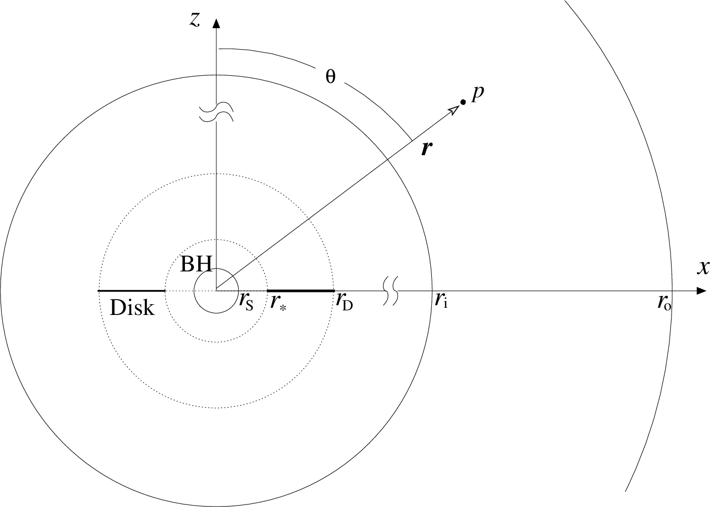
We mainly follow the methods used in the axisymmetric models by Proga et al. [84] and Proga & Kallman [82], and extend the problems to a full 3-D. Our basic model configuration is shown in Figure 1. The model geometry and the assumptions of the SMBH and the disk are very similar to those in Paper I, Paper II and Kurosawa & Proga [50]. For the simulations in 3-D, a SMBH with its mass and its Schwarzschild radius is placed at the center of the spherical coordinate system (, , ). The X-ray emitting corona regions is defined as a sphere with its radius , as shown in the figure. The geometrically thin and optically thick accretion disk (e.g., Shakura & Sunyaev 89) is placed on the equatorial plane ( plane). The 3-D hydrodynamic simulations will be performed in the spherical coordinate system with between the inner boundary and the outer boundary . For 2-D models, the -axis in the figure becomes the symmetry axis, and the computations are performed on plane. The radiation forces, from the corona region (the sphere with its radius ) and the accretion disk, acting on the gas located at a location () are assumed to be only in radial direction. The magnitude of the radiation force due to the corona is assumed to be a function of radius only, but that due to the accretion disk is assumed to be a function of and the polar angle which is the angle between the -axis and the position vector as shown in the figure. The point-source like approximation for the disk radiation pressure at is used here since the accretion disk radius ( in Fig. 1) is assumed to be much smaller than the inner radius, i.e., . In the following, we will describe our radiation hydrodynamics, our implementation of the radiation sources (the corona and disk), and radiative cooling/heating. Finally, we will also describe the model parameters and assumptions.
II.2. Hydrodynamics
We employ 3-D hydrodynamical simulations of the outflow from and accretion onto a central part of AGN, using the ZEUS-MP code [34, c.f.,] which is a massively parallel MPI-implemented version of the ZEUS-3D code (c.f., Hardee & Clarke 32; Clarke 16). The ZEUS-MP is a Eulerian hydrodynamics code which uses the method of finite differencing on a staggered mesh with a second-order-accurate, monotonic advection scheme [34]. To compute the structure and evolution of a flow irradiated by a strong continuum radiation of AGN, we solve the following set of HD equations:
| (1) |
| (2) |
| (3) |
where , , and are the mass density, energy density, pressure, and the velocity of gas respectively. Also, is the gravitational force per unit mass. The Lagrangian/co-moving derivative is defined as . We have introduced two new components to the ZEUS-MP in order to treat the gas dynamics more appropriate for the gas flow in and around AGN. The first is the acceleration due to radiative force per unit mass () in equation (2), and the second is the the effect of radiative cooling and heating simply as the net cooling rate () in equation (3). In our previous 3-D models (Kurosawa & Proga 50), we considered a simpler case with , but here we generalize the problem and consider cases with . We assume the equation of state to be in the form of where is the adiabatic index, and for all the models presented in this paper. Our numerical methods used in this paper are identical to, in most aspects, those described in Paper I and Paper II. In the following, we describe only the key elements of the calculations. Readers are referred to Paper I and Paper II (see also Proga et al. 84) for details.
Because of the accretion disk geometry (flat) which irradiates the surrounding gas, the flows in our models will not be spherically symmetric. The disk radiation flux, peaks in the direction of the disk rotational axis, and it gradually decreases as the polar angle increases, i.e., . The flow is also irradiated by a corona which is assumed to be spherical. The gas is assumed to be optically thin to its own cooling radiation. The following radiative processes are considered: Compton heating/cooling, X-ray photoionization heating, and recombination, bremsstrahlung and line cooling. We take into account some effects of photoionization on radiation pressure due to lines (line force). The line force is computed from a value of the photoionization parameter (defined as where and are the local X-ray flux and the number density of the gas) in combination with the analytical formulae from Stevens & Kallman [91]. The attenuation of the X-ray radiation by computing the X-ray optical depth in the radial direction is included. On the other hand, we do not include the attenuation of the UV radiation, to be consistent with our gas heating rates in which we include the X-ray photoionization but not UV photoionization. The method described above is found to be computationally efficient (cf. Paper I and Paper II), and provides good estimates for the number and opacity distribution of spectral lines for a given without detail information about the ionization state (see Stevens & Kallman 91).
Further, we assume that the total accretion luminosity consists of two components: (1) due to the accretion disk and (2) due to the corona. We assume that the disk emits only UV photons, whereas the corona emits only X-rays, i.e., the system UV luminosity, and the system X-ray luminosity, (in other words and ).
With these simplifications, only the corona radiation is responsible for ionizing the flow to a very high ionization state. While the corona contributes to the radiation force due to electron scattering in our calculations, it does not contribute to line driving. Metal lines in the soft X-ray band may have an appreciable contribution to the total radiation force in some cases. The disk radiation contributes to the radiation force due to both electron and line scattering.
II.3. Gas Rotation
For the simulations with gas rotation, we consider the accretion of gas with low specific angular momentum (). The low here means that the centrifugal force at large radii is small compared to gravity and gas pressure. Thus, at large radii and without radiation pressure, the flow is almost radial. However, at small radii, the flow starts to converge toward the equator, and it can eventually form a rotation–pressure supported torus like ones studied by e.g., Proga & Begelman [80] (in 2-D) and Janiuk et al. [38] (in 3-D). In general, gas at large radii would have a range of , and some fraction of gas would converge toward the equator even at large radii. On the other hand, some fraction of gas would have very small , and would directly fall onto the BH without going through a torus.
Following Proga & Begelman [80] and Paper II, we assume that the initial distribution of specific angular momentum , as a function of the polar angle , is
| (4) |
where is the specific angular momentum on the equator, and is a function monotonically decreases from to from the equator to the poles (at and ). Using the “circularization radius” (in the units of ) on the equator for the Newtonian potential (i.e., at ), the specific angular momentum on the equator can be written as:
| (5) |
where is used. The angular dependency in equation (4) is chosen as:
| (6) |
The initial rotational velocity () for the simulations are assigned as:
| (7) |
In this paper, we set which is smaller than the inner boundary radius (). This yields very weakly rotating gas which is far from a rotational equilibrium inside our computational domain. For example, the ratio of the centrifugal acceleration to the gravitational acceleration on the equator at the outer boundary () is only . We choose the relatively small value of to avoid a formation of a rotationally supported torus or disk in our computational domain and to avoid the complexities associated with it, e.g., the instability (in non-axisymmetric modes) of a torus found by Papaloizou & Pringle [70]. The low value of the gas specific angular momentum considered here allows us to study relatively simple flows, and to set an initial stage for modeling more complex flows associated with larger values of specific angular momentum, which shall be considered in a future study.
We assume that the circularized gas, which would be formed at (interior to the inner radius of our computational domain), will eventually accrete onto the SMBH on a viscous timescale. We do not model the actual process(es) of the angular momentum transport. A most likely mechanism of the angular momentum transport is magneto-rotational instability (Balbus & Hawley 4).
The formation of a torus wind, which might be associated with the X-ray “warm absorbers” (e.g., Lira et al. 53; Moran et al. 62; Iwasawa et al. 37; Crenshaw et al. 19; Blustin et al. 8) in Seyfert galaxies, are considered elsewhere (e.g., Dorodnitsyn et al. 24, Dorodnitsyn et al. 25). Here we are interested in a lager scale ( pc) weakly rotating wind which might be relevant to the NLR of AGNs. Readers are refer to Paper II for the axi-symmetric models with a different choice of the specific angular distribution function.
II.4. Model Setup
In all models presented here, the following ranges of the coordinates are adopted: , and (for 3-D models) where and . The polar and azimuthal angle ranges are divided into 128 and 64 zones, and are equally spaced. In the direction, the gird is divided into 128 zones in which the zone size ratio is fixed at .
For the initial conditions, the density and the temperature of gas are set uniformly, i.e., and everywhere in the computational domain where and throughout this paper (cf. Paper II). For the models without gas rotation, the initial velocity is set to zero everywhere. For the models with gas rotation, the initial velocity of the gas is assigned as described in § II.3 (see also Paper II).
At the inner and outer boundaries, we apply the outflow (free-to-outflow) boundary conditions, in which the field values are extrapolated beyond the boundaries using the values of the ghost zones residing outside of normal computational zones (see Stone & Norman 92 for more details). At the outer boundary, all HD quantities (except the radial component of the velocity, ) are assigned to the initial conditions (e.g., and ) during the the evolution of each model; however, this outer boundary condition is applied only when the gas is inflowing at the outer boundary, i.e., when . The radial component of the velocity is allowed to float (unconstrained) when at the outer boundary. For the models without gas rotation, is used for the outer boundary condition while equation (7) is used for those with gas rotation. Paper II also applied these conditions to represent a steady flow condition at the outer boundary. They found that this technique leads to a solution that relaxes to a steady state in both spherical and non-spherical accretion with an outflow (see also Proga & Begelman 81). This imitates the condition in which a continuous supply of gas is available at the outer boundary.
III. Results
We consider models with and without gas rotation in both 2-D and 3-D. The 2-D models are equivalent to Run C (without rotation) and Cr (with rotation) presented in Paper I and Paper II, but here we used the newly modified 3-D version of the code (ZEUS-MP). The 3-D models are equivalent to our 2-D models, but in those models, the assumption of the axisymmetry are dropped. We examine the differences and similarities of the 2-D and 3-D models, and investigate the importance of the non-axisymmetric natures of the flows in 3-D. The main parameters and results of the four models are summarized in Table 1. In the following, we describe the models results in detail.
 |
 |
 |
 |
III.1. Reference Values
| Rotation | |||||||||
|---|---|---|---|---|---|---|---|---|---|
| Model | |||||||||
| I | no | -10 | -1.8 | 8.0 | 94 | 0.01 | |||
| II | yes | -10 | -5.0 | 5.8 | 6.0 | 0.21 | |||
| III | no | -10 | -1.8 | 8.0 | 94 | 0.01 | |||
| IV | yes | -10 | -5.2 | 5.3 | 4.6 | 0.27 |
The following parameters are common to all the models presented here, and are exactly the same as in Paper I and Paper II. We assume that the central BH is non-rotating and has mass . The size of the disk inner radius is assumed to be (c.f. Sec. II.4). The mass accretion rate () of the central SMBH and the rest mass conversion efficiency () are assumed to be and , respectively. With these parameters, the corresponding accretion luminosity of the system is . Equivalently, the system has the Eddington number where and is the Eddington luminosity of the Schwarzschild BH, i.e., . The fractions of the luminosity in the UV () and that in the X-ray () are fixed at and respectively, as in Paper I (their Run C) and in Paper II (their Run Cr).
Important reference physical quantities relevant to our systems are as follows. The Compton radius, , is or equivalently where , and are the Compton temperature, the mean molecular weight of gas and the proton mass, respectively. We assume that the gas temperature at infinity is and . The corresponding speed of sound at infinity is . The corresponding Bondi radius [9] is while its relation to the Compton radius is . The Bondi accretion rate (for the isothermal flow) is . The corresponding free-fall time () of gas from the Bondi radius to the inner boundary is . The escape velocity from the inner most radius () of the computational domain is about .
 |
 |
 |
 |
 |
 |
 |
 |
III.2. Density, Temperature and Velocity Structures
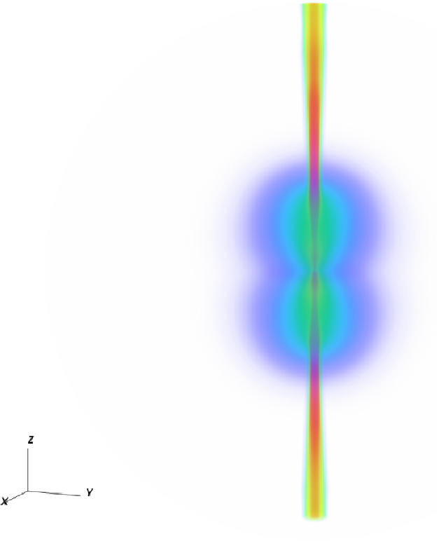
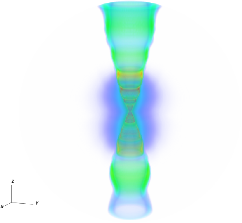
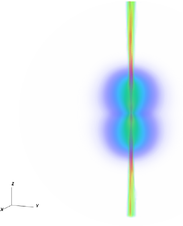
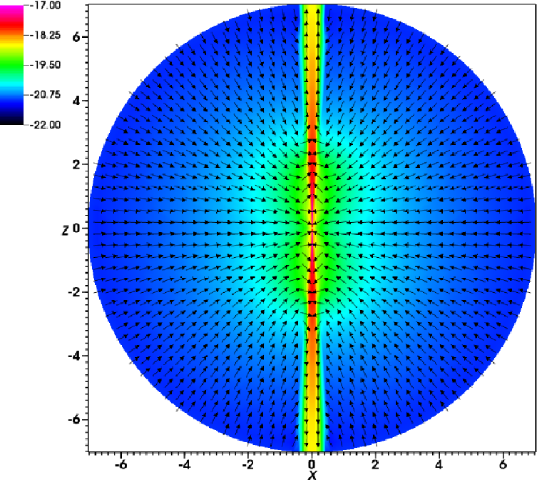
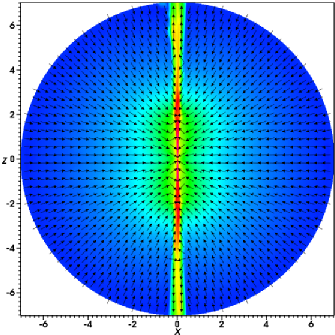
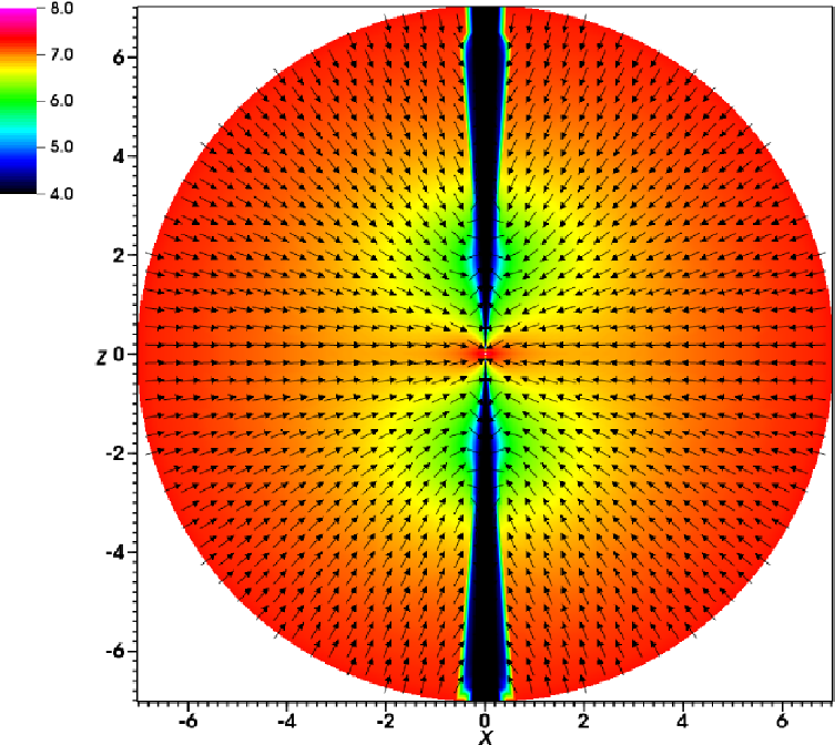
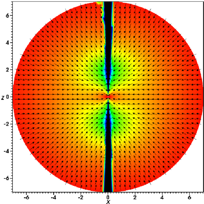
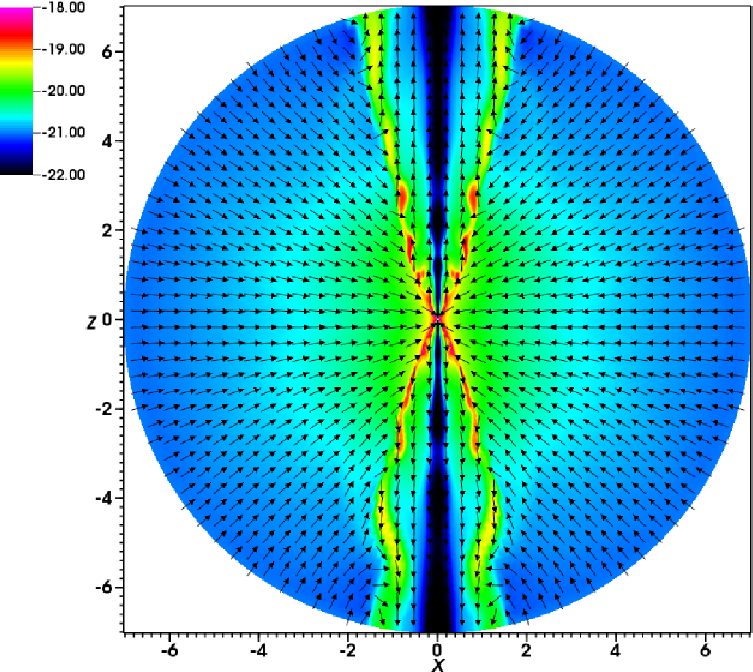
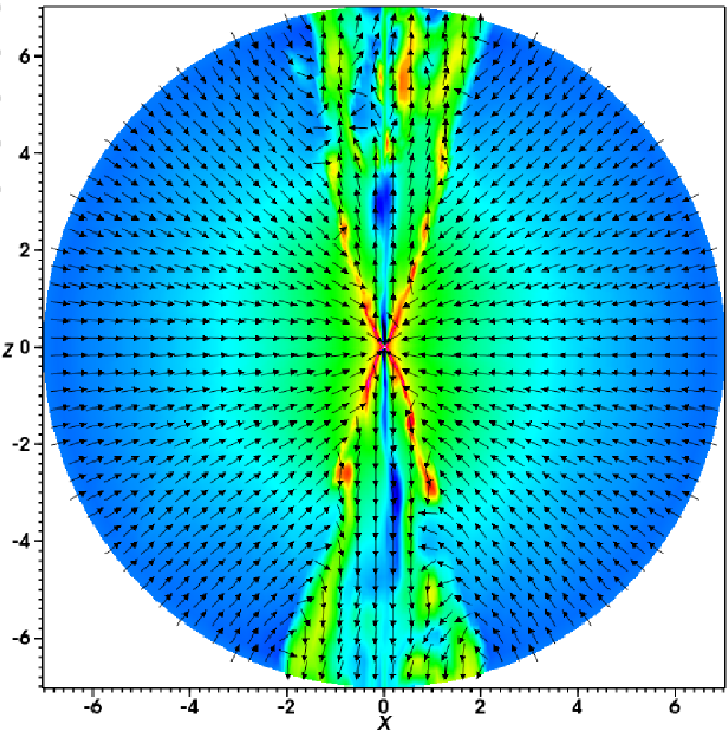
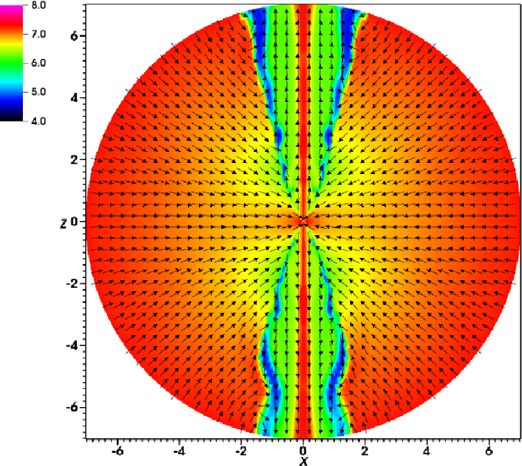
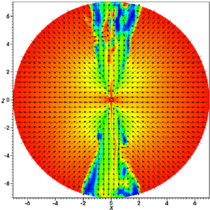
The 3-D representations of the density (as volume rendering images) of the models are shown in Figure 2. For the 2-D models, the density is extended around the -axis using the axisymmetry, to give 3-D views. The corresponding density and temperature maps along with the directions of the poloidal velocity of the flows on the – plane are given in Figures 3 and 4.
For non-rotating gas cases (Models I and III), the outflow occurs in very narrow cones in the polar directions (Figs. 2 and 3). The opening angles of the outflows in both models are about . The figures show that overall density structures of Models I and III are very similar to each other. Small but noticeable differences can be seen in the density structure in the narrow outflow regions. While the flow in Model I (2-D) is very smooth (steady), that of Model III (3-D) shows a hint of unsteadiness as indicated by the non-monotonic change of the density along the pole directions (unlike that of Model I). The increase of unsteadiness in the outflows of the 3-D model can be also seen in the variability of the mass outflow flux which we will discuss later in § III.3. Model III also shows a sign of non-axisymmetric flow although the degree of non-axisymmetry is rather small [ % variation of around the rotation axis for and (cf. § III.4)]. This can be clearly seen in the density (Fig. 3) of the narrow cones near the outer boundary where the density across a horizontal line is not symmetric with respect to the poles (the -axis). In spite of the small non-axisymmetry and variability of the internal structure of the narrow outflow cones, we find the overall structure or the integrity of the narrow outflow cones are intact, i.e., we find no wiggling of the cones themselves.
The gas rotation dramatically changes the morphology of the outflows. The centrifugal force due to gas rotation evidently pushes outflows away from the polar axis, and forms much wider outflows (less collimated), as seen in Figures 2 and 4. The opening angles of the outflows in both models are approximately . While the density is relatively high in the polar directions for the non-rotating models (Models I and III), it is relatively low for the rotating models (Models II and IV). The higher density regions (for the rotating cases) occur on and near the conic surfaces formed both above and below the equatorial planes. Similarly, the temperature along the poles is relatively low for the non-rotating cases, but it is relatively high for the rotating cases, especially in 2-D cases. Essentially the same differences between the models with and without gas rotation are found by of Paper II, cf., their run C and Cr.
As also observed in the model of Paper II, we find the outflows in the rotating cases tend to be fragmented into smaller pieces which have relatively high density and relatively low temperature (see Fig. 4). We find that these cold “cloud-like” features are formed around , and they flow outward along the outflow conic surface. We also find that the clouds (adiabatically) cool and expand as they move outward (see § III.5). Fig. 4 of Paper II, showing a time-sequence of density maps, demonstrates the motion of the cold outflow. The fragmentation of the outflow in the models with gas rotation (Model II and IV) is caused by a rapid radiative cooling of a high density gas which is formed at location where the inflow turns into the outflow, and the geometry of the outflow (the curved shape) which allows for a quite direct exposure to the strong X-ray from the central source. Readers are referred to Paper II for a more detailed explanation for the cause of fragmentation.
This cloud-like feature seen in the 2-D maps, of course, will look like rings if the density is rotated around the symmetry axis, as seen in the 3-D representation of the 2-D model with gas rotation (Model II in Fig. 2). In the 3-D model with rotation (Model IV in Fig. 2), we find that this ring structure is not stable. The ring tends to be deformed and breaks connections, due to shear and thermal instabilities. The parts of the broken ring structure also have relatively high density and low temperatures. They also resembles rather elongated cold cloud-like structures. Although the overall density and temperature structure of the flows in 2-D and 3-D for rotating cases are very similar to each other, the outflows occur in much less organized manner in the 3-D model.
III.3. Mass and Energy Flux
To examine the characteristics of the flows in the models more qualitatively, we compute the mass fluxes as a function of radius. For the 3-D models, the net mass flux (), the inflow mass flux () and the outflow mass flux () are computed by following Paper I (see also Kurosawa & Proga 50),
| (8) | ||||
| (9) |
where is the radial component of velocity . The net mass flux is obtained in the equation above if all are included. Similarly, the inflow mass flux and the outflow flux are obtained if only the points with and with are included, respectively, in the integration. The surface element and the solid angle element are and . We further define the outflow power in the form of kinetic energy () and that in the thermal energy () as functions of radius, i.e.,
| (10) |
and
| (11) |
where . For the 2-D models, the integrations are performed by assuming the axi-symmetry.
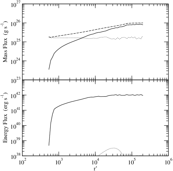
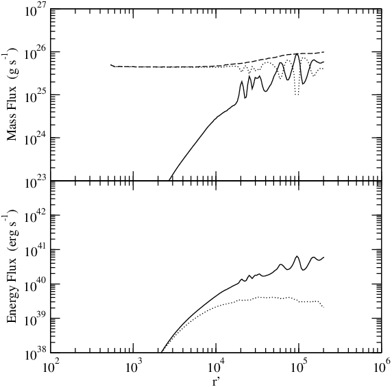
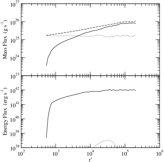
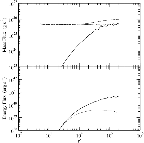
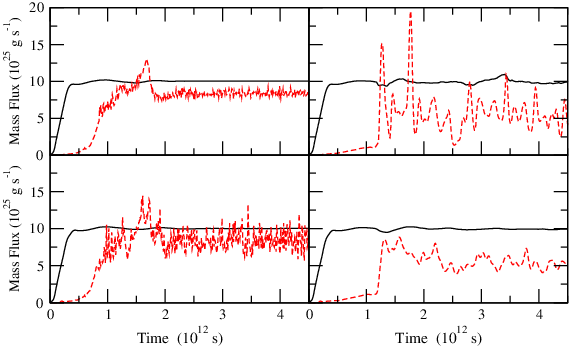
The resulting mass fluxes and the outflow powers of the models are summarized in Figure 5. In all cases, the mass inflow flux () exceeds the mass outflow rate () at all radii, except for the one point at for Model II. For Models I, III and IV, the net mass fluxes () are almost constant at all radii, indicating that the flows in these models are almost steady. A relatively steady nature of the flows in these models can be also seen in the time evolution of the mass inflow and outflow fluxes at the outer boundary, i.e., and , as shown in Figure 6.
We find that the radial dependencies of , and (Fig. 5) of Model III (3-D) are also almost identical to those of Model I (2-D). In § III.2, we found a hint of non-uniform density variation along the narrow outflow cones in the polar directions for the 3-D non-rotating case (Model III). As one can see from Figure 6, the time variability in for Model III is slightly higher than that of the 2-D mode (Model I). However, we find that the time averaged values (between and s) of for the non-rotating models (Models I and III) are almost identical to each other.
On the other hand, the 2-D rotating case (Model II) in Figure 5 shows a non-uniform distribution of for . This is caused by the non-uniform distribution of the outflow mass flux in , but not by that the inflow mass flux which has a smooth distribution across all radii. The non-uniform distribution of (bumps) is caused by the presence of the cold cloud-like (Fig. 4) or ring-like (Fig. 2) structures in the outflow. This also leads to a relatively large time variability in the outflow mass flux at the outer boundary for Model II, as shown in Figure 6. Interestingly, the bumps in seen in Model II (Fig. 5) are much less prominent in the 3-D equivalent of this model (Model IV). As mentioned before, the very organized ring-like structures seen in the outflows of the rotating 2-D model (Model II) tend to be stretched and fragmented in both radial and azimuthal directions (cf., Fig. 2). The outflow becomes much less organized. This results in the smoothing of the bumps on the curve in Figure 5 for the 3-D model (Model IV). This also causes the decrease in the degree of the time-variability in the mass outflow flux at the outer boundary, , as seen in Figure 6. Except for the bumps, overall behaviors of the mass flux curves (as a function of radius) of Model IV are very similar to those of the 2-D model, Model II. This shows that dimensionality does not change the gross properties of radiation-driven winds, and is consistent with the results of Proga [77] who studied radiation-driven winds in 1-D and 2-D.
The net mass fluxes at the inner boundary are , , and (or equivalently , , and ) for Models I, II, III and IV respectively (Tab. 1). This indicates that the net mass flux inward (negative signs indicate inflow) significantly increases when the gas is rotating (Models II and IV). We also find that the inflow mass fluxes at the outer boundary are same for all models (), but the outflow fluxes at the outer boundary decreases when the gas rotates (Tab. 1). The ratios of the total mass outflow flux to the total mass inflow flux at the outer boundary () are , , and for Models I, II, III and IV. These values indicate that relatively high efficiency of the outflow production by the radiation for . Interestingly, this conversion efficiency (from the outflow to inflow) becomes smaller for the models with gas rotations (Models II and IV).
Figure 5 also shows the outflow powers ( and ) of the models as a function of radius, as defined in eqs. (10) and (11). As in the mass flux curves in the same figure, the dependency of the energy flux on radius for the non-rotating cases (Models I and III) is almost identical to each other. Also for the rotating cases (Models II and IV), and curves are very similar to each others except for the small bumps around seen in the 2-D model (Model II), but not in the 3-D model (Model IV). The figure shows that in all four models, the outflow power is dominated by kinetic process although the difference between the kinetic power and the thermal power is much smaller than in the models with gas rotation. In other words, the kinetic power or the radiation force is more significant than the pressure gradient force in these models. We also find that the kinetic powers at the outer boundary dramatically decreases (more than an order of magnitude) when the gas is rotating (Models II and IV), but the thermal power at the outer boundary dramatically increases when the gas is rotating (cf., Tab. 1). No significant difference in the amount of and between 2-D and 3-D models is found.
In summary, we find that the rotation reduces the outflow collimation, and the outflow fluxes of mass and kinetic energy. Rotation also leads to fragmentation and time variability of the outflow, but this effect is reduced in the 3-D model (Model IV) as the ring-like structure seen in the 2-D model (Model II) becomes distorted and the flow becomes less organized. Rotation increases the outward flux of the thermal energy also. Finally, the rotation does not change the mass inflow rate through the outer boundary.
 |
 |
 |
 |
III.4. Non-axisymmetric Nature of the Flows in 3-D
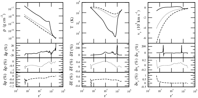
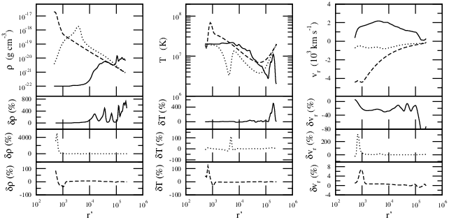
Next, we compare the difference between the 2-D and 3-D models more quantitatively. Figures 7 and 8 show the gas density (), temperature () and the radial velocity () of the 3-D models with no gas rotation (Model III) and with gas rotation (Model IV), respectively. The figures show that values of , and along three different polar angles (, , and ), but averaged over azimuthal angle , in order to compare the lines with those of the 2-D models (Models I and II, respectively). The figures also show the percentage differences between the 2-D and 3-D models.
For the non-rotating cases (Fig. 7), the percentage differences of , and between the 2-D and 3-D models are quite small ( %) along relatively larger polar angles, i.e., and , indicating the flow in along these lines are almost axi-symmetric. The difference becomes much larger along line as it is very close to the the region influenced by the outflow in which the effect of the radiative force is strongest.
As one can clearly see from the 3-D representation of the density distribution (Fig. 2), the deviation from the axisymmetry is much larger in the rotating cases. Figure 8 shows that the percentage differences of , and values between the 2-D and 3-D models (Models II and IV) along the three polar angles become very large ( %) at some radii, and they appear as sharp peaks or dips. These peaks and dips in the percentage difference plots are caused by the presence of the cold cloud-like structures which are stretched and drifted from the original ring-like structures (as seen in the 2-D model, cf. Fig. 2).
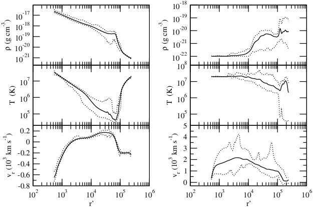
To demonstrate the amount of azimuthal variations in density, temperature and radial velocity in the 3-D models, we simply find their minimum and maximum values around the symmetry axis (-axis) for a fixed polar angle as a function of radius, and compared them with the azimuth angle averaged values. The results are shown in Figure 9 for the lines along the fixed polar angle of . Both models (Models III and IV) show clear signs of azimuthal variation hence the sings of non-axisymmetry at all radii. For the non-rotating case (Model III), the azimuthal variations of , and are largest in a mid section (–) while they tend to increase as increases for the rotating case (Model IV), except for that of which shows rather large variation at all radii. The overall azimuthal variations of , and in the rotating model are larger than those of the non-rotating model, indicating that the degree of non-axisymmetry is larger for the rotating case (Model IV). This is caused by the increase in the amount of shear and thermal instabilities in the models with gas rotation.
III.5. Properties of Gas — Photoionization Parameter, Temperature, and Radial Velocity
The volume averaged density () and temperature () of the gas in all four models are about and , and there is no significant difference between the models. The volume averaged values of photoionization parameters () are , , , and for Models I, II, III, and IV respectively. Again, no significant difference between the models is seen. As expected, the global properties of , and seem to be mainly controlled by the outer boundary conditions ( K and ) and the accretion luminosity, which are common to all the models presented here. In the following, we examine the property of the gas in each model more closely.
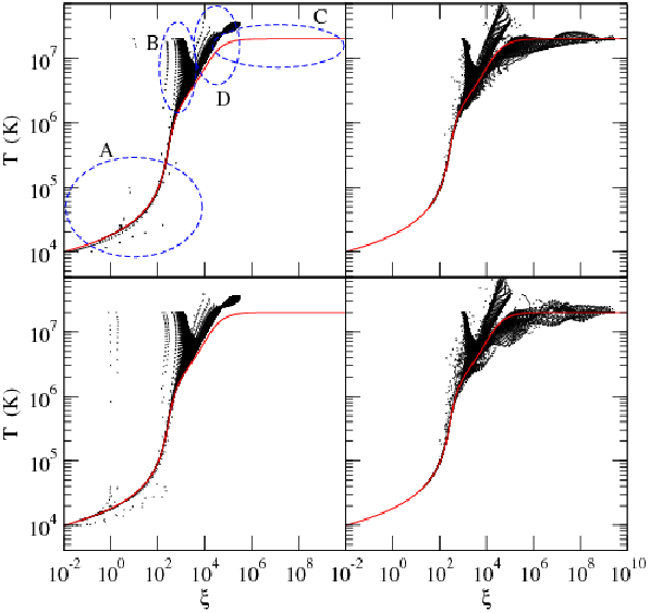
The scatter plots of the temperature of the gas as a function of the photoionization parameter for the models are shown in Figure 10 along with the cooling curve (assuming the radiative equilibrium) used in our model [see eq. (18) in Proga et al. 84 or Paper I]. For the 3-D models, only the points from the plane (cf., Figs. 3 and 4) are shown in the figure to avoid over-crowding of the points. Although the points from other planes are not shown here, by visual inspections we find that the points shown here represent the distributions of the whole samples.
The figure shows that the overall distributions of the points on the – planes from the 2-D models are very similar to those of the 3-D models. No significant difference between Models I and III is found, and neither between Models II and IV. On the other hand, the difference between the non-rotating cases (Models I and III) and the rotating cases (Models II and IV) are clearly seen. The – planes in the figures are divided into four main Regions (A, B, C and D). Although not shown here individually, close inspections of the points, by separating them with different ranges of , and the distance from the central source (), we found the following.
Region A. The points in this region are mainly found in the models without gas rotation (Models I and III). The gas in this region has relatively low temperatures ( K), and has relatively low values of photoionization parameter (). They are found at relatively small radii pc or equivalently , and have relatively large density (). They are outflowing gas with relatively large radial velocities ().
Region B. The points in this region are found in both models with (Models I and III) and without (Models II and IV) gas rotation. The temperature of the gas is relatively high ( K), and have median values of photoionization parameter (). They are found at relatively large distance from the center ( pc), and have relatively small density (). The gas in this region is mainly inflowing with relatively small radial velocities ().
Region C. The points in this region are mainly found in the models with rotations. The temperature of the gas is relatively high ( K), and have relatively high values of photoionization parameter (). The points in this region are found at relatively small radius ( pc), and have relatively low density (). The gas in this region is outflowing with relatively large radial velocity (), and is found mainly near the rotation axis. The property of the outflowing gas found here (in rotation cases) is very different from that of the outflowing gas in the non-rotating cases (Region A).
Region D. The points in this regions are found in both non-rotating and rotating cases, but a larger fraction of points are found in the rotating cases. The temperature of the gas is relatively high ( K), and have median values of photoionization parameter (). The points in this region are found at relatively small radius ( pc), and have relatively high density (). The gas in this region is inflowing with relatively large radial velocity ().
From the close inspection of the different regions mentioned above, we find that the deviations of the points on the – plane from the cooling curve are caused either by the compression/expansion or by the outer boundary conditions. The points in Region D, which are found above the cooling curve, are over-heated by the compression of the gas, as we found that the gas in this region is inflowing. In Region B, the gas is not in the radiative equilibrium because the gas is located at large radii and its thermal properties are influenced by the outer boundary condition, i.e., K regardless of . Further, the points in Region C, which are found in the outflow of the rotating models and located mostly just below the cooling curve, are slightly under-heated due to the influence of thermal expansion of the gas. Lastly, we find that the points in Region A, which are mainly in the non-rotating cases (Models I and III), mostly follow the cooling curve even though the points in regions are found to the relatively high speed outflow. This is because the outflow in the non-rotating models are mainly caused by the radiative pressure, but not due to thermal expansion, as we found in the energy power flux plot earlier in § III.3 (Fig. 5) whereas the thermal power is comparable to the kinetic power for the rotating cases.
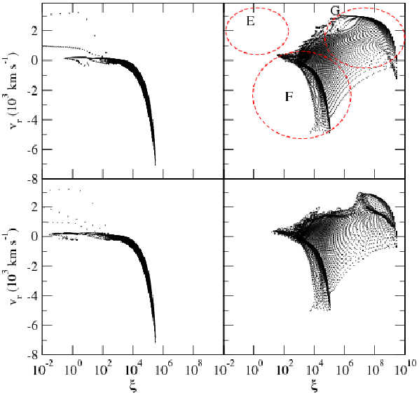
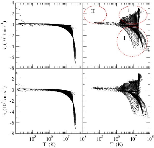
To see the difference in the properties of the outflowing gas between the non-rotating and rotating cases, the scatter plots of vs and vs of the four models are shown in Figures 11 and 12, respectively. Both – and – planes are divided into three distinctive regions (Regions E, F and G in Fig. 11; Regions H, I and J in Fig. 12).
As in the previous vs scatter plots, the distribution of the points are very similar between the 2-D and 3-D models. A small difference between the 2-D and 3-D models is seen in Region G (Fig. 11) of the rotating cases. The points for the inflowing gas () form a very similar pattern on the – plane (Region F in Fig. 11) for both rotating and non-rotating cases. The largest inflow speed of the gas is slightly higher in the non-rotating models, i.e., for the non-rotating models, and for the rotating models. A very noticeable difference between the rotating and the non-rotating cases is seen in the outflowing gas (). For the rotating models, the outflowing gas mainly appears in Region G where the photoionization parameter values are relatively high () while for the non-rotating cases, it mainly appears in Region E where the photoionization parameter values are relatively small (). Again, this is due to the difference in the dominating outflow mechanisms between the non-rotating and the rotating cases, i.e., the outflow is mainly radiatively driven for the non-rotating cases while the thermal pressure significantly contributes to the outflows of the rotating cases (cf. Fig. 5).
Rather similar patterns of the scattered points (to those in the ) are seen in the – plane (Fig. 12). Again, the planes are divided into three regions (Regions H, I and J), and no significant difference between the distributions of the points in the 2-D and the 3-D models is seen. The points for the inflowing gas appear in Region I in the rotating and the non-rotating cases, and their distributions are somewhat similar to each other. For the rotating models, the outflowing gas mainly appear in Region J where the gas temperatures are relatively high ( K) while for the non-rotating cases, they mainly appear in Region H where the temperatures are relatively small ( K).
By comparing the physical properties of different regions in Figures 10, 11 and 12, we found the following connections among them. Regions A, E and H are likely to belong to same grid points (same spatial locations). Region B corresponds to the upper section of Region F. The points in Regions C, G and J are also likely to belong to same grid points, so do the points in Regions F and I, respectively.
IV. Discussions
IV.1. Virial Mass and Cold Clouds
To understand the evolution of galaxies which is greatly influenced by the existence and the growth rate of the central SMBH, accurate measurements of fundamental physical quantities such as mass of a SMBH are important. While it is possible to estimate the masses directly from the kinematics of the gas and stars for nearby systems, it is difficult/impossible to apply this method for more distant objects and for a very large number of objects (cf. a review by Ferrarese & Ford 30). For the distant objects, the masses are estimated by the reverberation mapping technique (cf. a recent review by Peterson & Bentz 73) in conjunction with the virial theorem, i.e.,
| (12) |
where and are the average speed of an ensemble of the line emitting clouds and the average distance of the ensemble of line emitting clouds from the center.
The mass estimate via the virial theorem uses the assumption that the line emitting regions are gravitationally bounded and the outflows are negligible. This assumption is not quite valid for the system with relatively high Eddington number (), as this is the case for our models (). The outflow motions of gas are clearly observed in our simulations too. In case of a point-source approximation (for radiation source), the radiation force scales as (so does the gravitational force). Hence, the effective gravity (including the radiation force term) will be reduced. Consequently, the masses computed from the virial theorem will underestimate actual masses, for the system with relatively large . This effect may be especially important for the Seyfert galaxies with high [O III] 5007 blueshifts (“blue outliers”) which deviates from the – relation of normal, narrow-line Seyfert 1 (NLS1) and broad-line Seyfert 1 (BLS1) galaxies (Komossa & Xu 42; Komossa et al. 43). A recent work by Marconi et al. [59] explicitly demonstrates that the correction for the virial mass estimate is significant when one include the effect of radiation force (see also Peterson & Wandel 74; Krolik 49; Onken & Peterson 68; Collin et al. 17; Vestergaard & Peterson 95).
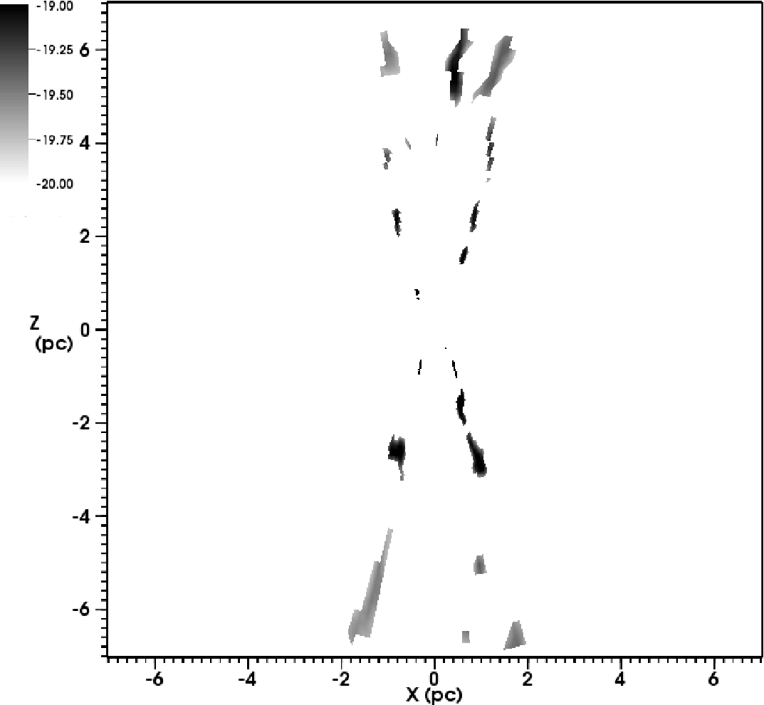
We apply the virial theorem to our simulation result to estimate the BH mass in spite of the obvious outflows seen in our simulations, and compare the value with the actual mass used in the simulation. We restrict our discussion to the results of the 3-D model with gas rotation (Model IV). We assume the lines are formed in the dense cold-cloud like structures, which might resemble the narrow-line regions (NLR) of AGN (found in § III.2). The velocities and positions of the cloud elements (the model grid points which belong to the clouds) will be used in the virial theorem. We define the gas to be in dense cold-cloud state when its density is higher than and its temperature is less than .
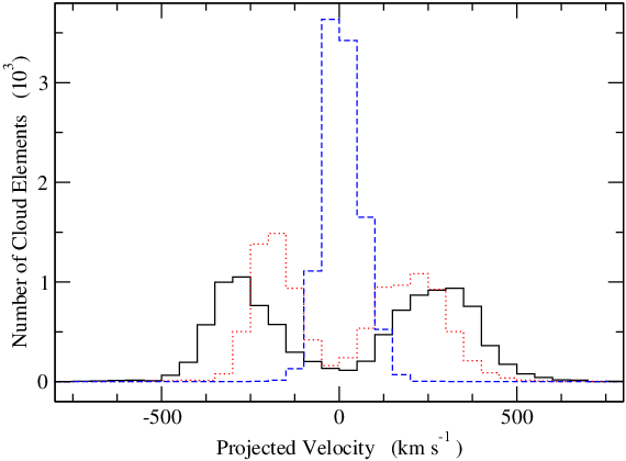
Figure 13 shows the morphology of the cloud distribution on the – plane. The projected velocities () of the cold cloud elements to an observer, located at the inclination angles , and , are shown in Figure 14. The figure shows that the distributions of for the lower inclination angles ( and ) display double peaks, and their separation decreases as the inclination angle increases. These are expected features from the bi-conic outflow geometry (as in Figs. 4 and 13).
To compute the virial mass, we compute the average speed of the cold cloud directly from our simulation result, i.e., where and are the speed of an individual cold cloud element and the total number of the clouds, respectively. Similarly, the average radial distance is computed as where is the radial distance of an individual cloud element. For Model IV, we find and . Note that the escape velocity of the cold clouds, from the cloud forming radius () in Model IV, is about which is much larger than the average speed of the clouds (). The corresponding viral mass, using equation (12), is which is about % smaller than the actual mass of the BH used in the simulation, i.e., . This is in general agreement with the previous statement: the virial mass determined using equation (12) would underestimate actual mass for systems with relatively high in which the radiation force is comparable to or greater than the gravitational force. A systematic correction for the radiation force in the virial mass estimate, in general, is very challenging since the radiation force (line force) depends on the ionization state of the gas, and its strength is not spherically symmetric. Further, the outflow geometry is non-spherical, and it depends on the rotation rate of the gas (cf. Models III and IV in Fig. 2).
IV.2. Comparisons with Observations of Seyfert Galaxies
The studies of kinematics in the NLR of Seyfert galaxies will provide us a hint for understanding the complicated dynamical processes and the driving forces (radiation, magnetic or thermal) in their vicinity. The NLR of nearby Seyfert galaxies are especially useful for testing outflow models since they can be spatially resolved (e.g., Evans et al. 27; Macchetto et al. 58; Hutchings et al. 36; Nelson et al. 66; Crenshaw et al. 20; Crenshaw & Kraemer 18; Ruiz et al. 86; Cecil et al. 12; Ruiz et al. 87; Das et al. 23, Das et al. 22; Kraemer et al. 47; Walsh et al. 96). In particular, the Faint Object Camera (FOC) and the Space Telescope Imaging Spectrograph (STIS) on HST, allow for detailed constraints on the kinematics of the NLR in Seyfert galaxies. For example, using the STIS, Das et al. [23] obtained the position dependent spectra of [O III] for NGC 4151, one of the closest Seyfert galaxies, with different long slit positions, and studied the kinematics of the wind in the NLR by measuring its projected velocity components from the position of multiple peaks (up to three peaks) in the [O III] profiles. Their results are very intriguing. For scales from 10 pc to 100 pc, they found that the velocity increases nearly linearly with radius whereas at larger scales, the velocity decreases, again nearly linearly, with increasing radius. Spatially resolved observations of the NLR in other AGN show similar flow patterns (e.g., NGC 1068: Crenshaw et al. 20; Kraemer & Crenshaw 46 and Mrk 3: Ruiz et al. 87).
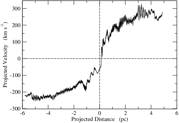
To compare our model with the kinematics study of NGC 4151 Das et al. [23], we compute the velocity of the cold clouds (as defined in § IV.1) in Model IV (cf. Fig. 13) projected () toward an observer at the inclination angle , which is also the inclination of NGC 4151 (Das et al. 23). Das et al. [23] used that the kinematics model of the outflows with a bi-conic radial velocity law, and found a good fit to their observations when the opening angle of the cone is . Interestingly, we find the opening angle of the outflows in Model IV is also about (cf. Figs. 2 and 4).
Figure 15 shows of the clouds plotted as a function of the projected vertical distance, which is the distance along the -axis in Fig. 13 projected onto the plane of the sky for an observer viewing the system with . The figure shows that the clouds are accelerated up to until the projected distance reaches pc, but the velocity curve starts to flatten beyond this point. Towards the outer edges (near the outer boundaries), the curve begins to show a sign of deceleration, but not so clearly. We note that the hot outflowing gas, on the other hand, does show deceleration at the larger radii in our models (cf. Fig. 9). Although the physical size of the long slit observation of NGC 4151 by Das et al. [23] is in much lager scale ( times larger) than that of our model, their radial velocities as a function of the position along the slit (see their Figs. 5 and 6) show a similar pattern as in our model (Fig. 15). The range of in our model is about to while the range of the observed radial velocities in Das et al. [23] is about to , which is comparable to ours. To understand the large scale outflows seen in the observations and to understand the kinematics of such outflows better, the size of the simulation box must be increased at least by a factor of 100. In such larger scales, the temperature is expected to be much cooler, and the dust would play an important role in determining the thermal and dynamical properties the outflows (e.g. Antonucci 1; Miller & Goodrich 61; Awaki et al. 3; Blanco et al. 6; Krolik 48). These are beyond the scope of this paper, but shall be considered in a future paper.
V. Conclusions
We have presented the dynamics of gas under the influences of the gravity of a SMBH and the radiation force from the luminous accretion disk around the SMBH. This is a direct extension of the previous axi-symmetric models of Paper I and Paper II to a full 3-D model, and is an extended version of the models presented in Kurosawa & Proga [50] to which we have added the radiation force due to line processes and the radiative cooling and heating effect. We have considered two cases from Paper I and Paper II: (1) the formation of outflow from the accretion of the ambient gas with no rotation and (2) that with weak rotation. The models have been considered in both 2-D and 3-D hence, in total, four models have been presented. Our first main goal is to examine if there is a significant difference between two models with identical initial and outer boundary conditions but in different dimensionality (2-D and 3-D). In particular, we examine whether the radiation driven outflows that were found to be stable in the previous studies in 2-D (Paper I; Paper II) still remain stable in 3-D. Our second main goal is to gain some insights into the gas dynamics in AGNs and Seyfert galaxies by comparing the simulation results with observations. In the following, we summarize our main findings through this investigation.
1. For non-rotating gas cases, the outflow occurs in very narrow cones (with the opening angles ) in polar directions. Overall density and temperature of the both 2-D and 3-D models (Models I and III) are very similar to each other (Figs. 2 and 3). Small but noticeable differences are seen in the narrow outflow regions.
2. Rotation of gas significantly changes the morphology of the outflows (Models II and IV in Figs. 2 and 4). The centrifugal force pushes the outflow away from the polar axis and forms much wider outflows (with the opening angles ). The outflow occurs mainly on and near bi-conic surfaces, and relatively low values of density are found in the polar directions, unlike the outflows in the non-rotating cases. The models with gas rotation show cold clouds (clumps) in their outflows in their 2-D density and temperature maps (Fig. 4). Although the overall density and temperature structures of the flows of the 2-D and 3-D models are similar to each other, the outflows in 3-D occur in much less organized manner. We find that the cloud-like structures seen in the 2-D model (Model II), which are rings if the density is expanded in 3-D using the axisymmetry (Fig. 2), are not stable in full 3-D simulations due to the shear and thermal instabilities. The rings break up into smaller pieces, and fully 3-D clouds are formed in Model IV.
3. The mass and energy fluxes plotted as a function of radius for the 3-D non-rotating case are almost identical to those of the non-rotating 2-D case (Fig. 5). For the rotating cases, the bumps seen in the mass-inflow rate and the net mass flux at the outer radii () for the 2-D model (Model II) are smoothed out in the 3-D model (Model IV) due to the fragmentation of the ring structures in the 3-D model. While the kinetic power dominates at all radii for the non-rotating cases, the thermal power contributes significantly to the outflow driving force for the rotating cases. In spite of the differences in the flow geometries, the rotating models in both 2-D and 3-D show very similar values of the mass accretion and outflow rates at the outer and inner boundaries (Table 1). In other words, AGN feedback due to radiation is similar in the 2-D and 3-D cases as far as the time-averaged mass and energy fluxes are concerned.
4. For the non-rotating cases, the amount of variability in the mass flux at the outer boundary is higher in the 2-D model than that in the 3-D model, but the opposite is true for the rotating cases (Fig. 6).
5. In the 3-D models, the deviations from the axisymmetry are observed in both rotating and non-rotating cases (Figs. 7 and 8). The amounts of the azimuthal angle variations of the density, temperature, and radial velocity (Fig. 9) are relatively small for the non-rotating case (Model III), but they are relatively large at all radii for the rotating case (Model IV).
6. The gas properties of the 2-D and 3-D models are very similar to each other for both non-rotating and rotating cases (Figs. 10, 11 and 12). The majority of the outflowing gas for the rotating cases (Models II and IV) has relatively large values of the photoionization parameter () while for the non-rotating cases, it has relatively small values of the photoionization parameters () (Fig. 11). This is due to the difference in the dominant outflow mechanisms between the non-rotating and the rotating cases, i.e., the outflow is mainly radiatively driven for the non-rotating cases while the thermal pressure significantly contributes to the outflows of the rotating cases (cf., Fig. 5). For the rotating models, the majority of the outflowing gas has relatively high ( K) temperature while for the non-rotating cases, it has relatively low ( K) temperature. The higher values seen in the rotating cases are mainly from the low-density hot outflowing gas in between the outflowing cold clouds.
7. For Model IV, we find the average speed and the radial position of the cold cloud elements (§ IV.1) as and . The corresponding viral mass is which is about 40 % smaller than the actual mass of the BH used in the simulation, i.e., . This is in general agreement with the previous studies (e.g. Peterson & Wandel 74; Krolik 49; Marconi et al. 59) which predict that the virial mass estimated without considering the effect of the radiation force underestimates the actual mass of the SMBH.
8. The opening angles () of the bi-conic outflows found in the the rotating models (Models II and IV) are very similar to that of the nearby Seyfert galaxy NGC 4151 () determined by Das et al. [23]. Although the physical size of the long slit observations of NGC 4151 by Das et al. [23] is in much lager scale ( times larger) than that of our model, their radial velocities as a function of the position along the slit (see their Figs. 5 and 6) show a similar pattern as in our model (Fig. 15). An important difference between the observation of Das et al. [23] and our models is the lack of clearly decelerating clouds at larger radii in our models. However, we note that the clouds found in our simulations reach a constant velocity near the outer boundary of our simulations, and show a hint of deceleration. This puzzling outflow deceleration seen in the observations might be due to the inflow that interacts with the polar outflows. The reason for no clear cloud deceleration seen in our model may be simply due to the relatively small simulation box size we used, and the issue could be resolved in a lager scale simulation. Spectroscopic studies of the NLR of Seyfert galaxies by Komossa et al. [43] also favor a scenario in which the NLR clouds are traveling in decelerating wind. The hot outflowing gas, on the other hand, does show deceleration at the larger radii in our models (cf. Fig. 9).
To perform a better comparison of our models with observations hence to constrain the model parameters, in future studies, we need to increase the size of the simulation box to match the physical sizes of the NLR of Seyfert galaxies. It would take the outer radius of the computational domain to be expanded by one or even two orders of magnitude compared to the one used here. The dust is very likely important in the dynamics of the outflow in the larger scale simulations since the temperature becomes low enough for the dust survival and formation in the larger radius. We showed in Paper II, relatively high density set at the outer boundary promotes formation of cold clouds. Therefore, we plan to explore the effects of dust and outer boundary density.
To compare the model results directly with observations, we would need to compute the radiative transfer models of the important emission lines (e.g., [O III] , H and C IV ), which will be the topic of our future paper. Taking these steps will allow a quite strict test of our results against observations of Seyfert galaxies and AGN. It would also be interesting to check if our models could reproduce large-scale outflows in quasars, for example the high-velocity outflow components seen in C IV and Mg II quasar absorption-line systems (e.g., see a recent work by Wild et al. 99) which would provide an additional constraint on our wind models.
References
- [1] Antonucci, R. R. J. 1984, ApJ, 278, 499
- [2] Arav, N., Li, Z.-Y., & Begelman, M. C. 1994, ApJ, 432, 62
- [3] Awaki, H., Koyama, K., Inoue, H., & Halpern, J. P. 1991, PASJ, 43, 195
- [4] Balbus, S. A. & Hawley, J. F. 1991, ApJ, 376, 214
- [5] Begelman, M., de Kool, M., & Sikora, M. 1991, ApJ, 382, 416
- [6] Blanco, P. R., Ward, M. J., & Wright, G. S. 1990, MNRAS, 242, 4
- [7] Blandford, R. D. & Payne, D. G. 1982, MNRAS, 199, 883
- [8] Blustin, A. J., Page, M. J., Fuerst, S. V., Branduardi-Raymont, G., & Ashton, C. E. 2005, A&A, 431, 111
- [9] Bondi, H. 1952, MNRAS, 112, 195
- [10] Bottorff, M., Korista, K. T., Shlosman, I., & Blandford, R. D. 1997, ApJ, 479, 200
- [11] Brighenti, F. & Mathews, W. G. 2006, ApJ, 643, 120
- [12] Cecil, G., Dopita, M. A., Groves, B., Wilson, A. S., Ferruit, P., Pécontal, E., & Binette, L. 2002, ApJ, 568, 627
- [13] Ciotti, L. & Ostriker, J. P. 1997, ApJ, 487, L105
- [14] —. 2001, ApJ, 551, 131
- [15] —. 2007, ApJ, 665, 1038
- [16] Clarke, D. A. 1996, ApJ, 457, 291
- [17] Collin, S., Kawaguchi, T., Peterson, B. M., & Vestergaard, M. 2006, A&A, 456, 75
- [18] Crenshaw, D. M. & Kraemer, S. B. 2000, ApJ, 532, L101
- [19] Crenshaw, D. M., Kraemer, S. B., Gabel, J. R., Schmitt, H. R., Filippenko, A. V., Ho, L. C., Shields, J. C., & Turner, T. J. 2004, ApJ, 612, 152
- [20] Crenshaw, D. M. et al. 2000, AJ, 120, 1731
- [21] Dalla Vecchia, C., Bower, R. G., Theuns, T., Balogh, M. L., Mazzotta, P., & Frenk, C. S. 2004, MNRAS, 355, 995
- [22] Das, V., Crenshaw, D. M., Kraemer, S. B., & Deo, R. P. 2006, AJ, 132, 620
- [23] Das, V. et al. 2005, AJ, 130, 945
- [24] Dorodnitsyn, A., Kallman, T., & Proga, D. 2008a, ApJ, 675, L5
- [25] —. 2008b, ApJ, 687, 97
- [26] Emmering, R. T., Blandford, R. D., & Shlosman, I. 1992, ApJ, 385, 460
- [27] Evans, I. N., Tsvetanov, Z., Kriss, G. A., Ford, H. C., Caganoff, S., & Koratkar, A. P. 1993, ApJ, 417, 82
- [28] Everett, J. E. & Murray, N. 2007, ApJ, 656, 93
- [29] Fabian, A. C., Sanders, J. S., Taylor, G. B., Allen, S. W., Crawford, C. S., Johnstone, R. M., & Iwasawa, K. 2006, MNRAS, 366, 417
- [30] Ferrarese, L. & Ford, H. 2005, Space Science Reviews, 116, 523
- [31] Fontanot, F., Monaco, P., Cristiani, S., & Tozzi, P. 2006, MNRAS, 373, 1173
- [32] Hardee, P. E. & Clarke, D. A. 1992, ApJ, 400, L9
- [33] Hawley, J. F. & Balbus, S. A. 2002, ApJ, 573, 738
- [34] Hayes, J. C., Norman, M. L., Fiedler, R. A., Bordner, J. O., Li, P. S., Clark, S. E., ud-Doula, A., & Mac Low, M.-M. 2006, ApJS, 165, 188
- [35] Hopkins, P. F., Hernquist, L., Cox, T. J., Di Matteo, T., Martini, P., Robertson, B., & Springel, V. 2005, ApJ, 630, 705
- [36] Hutchings, J. B. et al. 1998, ApJ, 492, L115
- [37] Iwasawa, K., Fabian, A. C., Almaini, O., Lira, P., Lawrence, A., Hayashida, K., & Inoue, H. 2000, MNRAS, 318, 879
- [38] Janiuk, A., Proga, D., & Kurosawa, R. 2008, ApJ, 681, 58
- [39] Kato, Y. 2007, Ap&SS, 307, 11
- [40] Kato, Y., Mineshige, S., & Shibata, K. 2004, ApJ, 605, 307
- [41] King, A. 2003, ApJ, 596, L27
- [42] Komossa, S. & Xu, D. 2007, ApJ, 667, L33
- [43] Komossa, S., Xu, D., Zhou, H., Storchi-Bergmann, T., & Binette, L. 2008, ApJ, 680, 926
- [44] Königl, A. 2006, Mem. Soc. Astron. Italiana, 77, 598
- [45] Königl, A. & Kartje, J. F. 1994, ApJ, 434, 446
- [46] Kraemer, S. B. & Crenshaw, D. M. 2000, ApJ, 544, 763
- [47] Kraemer, S. B., Schmitt, H. R., & Crenshaw, D. M. 2008, ApJ, 679, 1128
- [48] Krolik, J. H. 1999, Active Galactic Nuclei: From the Central Black Hole to the Galactic Environment (Princeton: Princeton Univ. Press)
- [49] —. 2001, ApJ, 551, 72
- [50] Kurosawa, R. & Proga, D. 2008, ApJ, 674, 97
- [51] Laor, A. & Draine, B. T. 1993, ApJ, 402, 441
- [52] Li, H., Lovelace, R. V. E., Finn, J. M., & Colgate, S. A. 2001, ApJ, 561, 915
- [53] Lira, P., Lawrence, A., O’Brien, P., Johnson, R. A., Terlevich, R., & Bannister, N. 1999, MNRAS, 305, 109
- [54] Lovelace, R. V. E., Wang, J. C. L., & Sulkanen, M. E. 1987, ApJ, 315, 504
- [55] Lynden-Bell, D. 1969, Nature, 223, 690
- [56] —. 1996, MNRAS, 279, 389
- [57] —. 2003, MNRAS, 341, 1360
- [58] Macchetto, F., Capetti, A., Sparks, W. B., Axon, D. J., & Boksenberg, A. 1994, ApJ, 435, L15
- [59] Marconi, A., Axon, D. J., Maiolino, R., Nagao, T., Pastorini, G., Pietrini, P., Robinson, A., & Torricelli, G. 2008, ApJ, 678, 693
- [60] McNamara, B. R., Nulsen, P. E. J., Wise, M. W., Rafferty, D. A., Carilli, C., Sarazin, C. L., & Blanton, E. L. 2005, Nature, 433, 45
- [61] Miller, J. S. & Goodrich, R. W. 1990, ApJ, 355, 456
- [62] Moran, E. C., Filippenko, A. V., Ho, L. C., Shields, J. C., Belloni, T., Comastri, A., Snowden, S. L., & Sramek, R. A. 1999, PASP, 111, 801
- [63] Murray, N., Chiang, J., Grossman, S. A., & Voit, G. M. 1995, ApJ, 451, 498
- [64] Murray, N., Quataert, E., & Thompson, T. A. 2005, ApJ, 618, 569
- [65] Nakamura, M., Li, H., & Li, S. 2006, ApJ, 652, 1059
- [66] Nelson, C. H., Weistrop, D., Hutchings, J. B., Crenshaw, D. M., Gull, T. R., Kaiser, M. E., Kraemer, S. B., & Lindler, D. 2000, ApJ, 531, 257
- [67] Ohsuga, K. 2007, ApJ, 659, 205
- [68] Onken, C. A. & Peterson, B. M. 2002, ApJ, 572, 746
- [69] Ostriker, J. P., Weaver, R., Yahil, A., & McCray, R. 1976, ApJ, 208, L61
- [70] Papaloizou, J. C. B. & Pringle, J. E. 1984, MNRAS, 208, 721
- [71] Park, M.-G. & Ostriker, J. P. 2001, ApJ, 549, 100
- [72] —. 2007, ApJ, 655, 88
- [73] Peterson, B. M. & Bentz, M. C. 2006, NewA Rev., 50, 796
- [74] Peterson, B. M. & Wandel, A. 2000, ApJ, 540, L13
- [75] Phinney, E. S. 1989, in Theory of Accretion Disks, ed. F. Meyer (NATO ASI Ser. C, 290; Dordrecht: Kluwer), 457
- [76] Pier, E. A. & Krolik, J. H. 1992, ApJ, 399, L23
- [77] Proga, D. 1999, MNRAS, 304, 938
- [78] Proga, D. 2007, ApJ, 661, 693 (Paper I)
- [79] Proga, D. 2007, in ASP Conf. Ser. 373, The Central Engine of Active Galactic Nuclei, ed. L. C. Ho & J.-W. Wang (San Fransisco: ASP), 267
- [80] Proga, D. & Begelman, M. C. 2003, ApJ, 582, 69
- [81] Proga, D. & Begelman, M. C. 2003, ApJ, 592, 767
- [82] Proga, D. & Kallman, T. R. 2004, ApJ, 616, 688
- [83] Proga, D., Ostriker, J. P., & Kurosawa, R. 2008, ApJ, 676, 101 (Paper II)
- [84] Proga, D., Stone, J. M., & Kallman, T. R. 2000, ApJ, 543, 686
- [85] Quilis, V., Bower, R. G., & Balogh, M. L. 2001, MNRAS, 328, 1091
- [86] Ruiz, J. R., Crenshaw, D. M., Kraemer, S. B., Bower, G. A., Gull, T. R., Hutchings, J. B., Kaiser, M. E., & Weistrop, D. 2001, AJ, 122, 2961
- [87] —. 2005, AJ, 129, 73
- [88] Sazonov, S. Y., Ostriker, J. P., Ciotti, L., & Sunyaev, R. A. 2005, MNRAS, 358, 168
- [89] Shakura, N. I. & Sunyaev, R. A. 1973, A&A, 24, 337
- [90] Springel, V., Di Matteo, T., & Hernquist, L. 2005, ApJ, 620, L79
- [91] Stevens, I. R. & Kallman, T. R. 1990, ApJ, 365, 321
- [92] Stone, J. M. & Norman, M. L. 1992, ApJS, 80, 753
- [93] Tremonti, C. A., Moustakas, J., & Diamond-Stanic, A. M. 2007, ApJ, 663, L77
- [94] Vernaleo, J. C. & Reynolds, C. S. 2006, ApJ, 645, 83
- [95] Vestergaard, M. & Peterson, B. M. 2006, ApJ, 641, 689
- [96] Walsh, J. L., Barth, A. J., Ho, L. C., Filippenko, A. V., Rix, H.-W., Shields, J. C., Sarzi, M., & Sargent, W. L. W. 2008, AJ, 136, 1667
- [97] Wang, J.-M., Chen, Y.-M., & Hu, C. 2006, ApJ, 637, L85
- [98] Weymann, R. J., Scott, J. S., Schiano, A. V. R., & Christiansen, W. A. 1982, ApJ, 262, 497
- [99] Wild, V. et al. 2008, MNRAS, 388, 227
- [100] Zanni, C., Murante, G., Bodo, G., Massaglia, S., Rossi, P., & Ferrari, A. 2005, A&A, 429, 399