Experimental test of nonclassicality criteria

T. Kiesel, W. Vogel Affiliation: Arbeitsgruppe Quantenoptik, Institut für Physik, Universität Rostock, D-18051 Rostock, Germany B. Hage, J. DiGuglielmo, A. Samblowski, and R. Schnabel Affiliation: Institut für Gravitationsphysik, Leibniz Universität Hannover and Max-Planck-Institut für Gravitationsphysik (Albert-Einstein-Institute),
Callinstrasse 38, 30167 Hannover, Germany

Abstract

We experimentally examine the nonclassical character of a class of non-Gaussian states known as phase-diffused squeezed states. These states may show no squeezing effect at all, and therefore provide an interesting example to test nonclassicality criteria. The characteristic function of the Glauber-Sudarshan representation ( $P$ function) proves to be a powerful tool to detect nonclassicality. Using this criterion we find that phase-diffused squeezed states are always nonclassical, even if the squeezing effect vanishes. Testing other criteria of nonclassicality based on higher-order squeezing and the positive semidefinitness of special matrices of normally ordered moments, it is found that these criteria fail to reveal the nonclassicality for some of the prepared phase-diffused squeezed states.

pacs

03.65.Wj, 42.50.Dv, 42.50.Xa

I Introduction

The definition of nonclassicality of a quantum state of the harmonic oscillator is closely connected to the coherent states. These are the eigenstates of the annihilation operator, $\hat{a}\left|\alpha\right>=\alpha\left|\alpha\right>$ , where the complex number $\alpha$ defines the amplitude and phase of the field [1]. Glauber and Sudarshan showed that the density operator of an arbitrary optical quantum state can be formally written as a statistical mixture of coherent states,

\hat{\rho}=\int d^{2}\alpha\,P(\alpha)\left|\alpha\right>\left<\alpha\right|,

(1)

where the Glauber-Sudarshan representation $P(\alpha)$ plays the role of the probability distribution of coherent states [2, 3]. However, in quantum optics $P(\alpha)$ often violates the properties of a probability density. Hence, a state is referred to as nonclassical if its $P$ function does not exhibit the properties of a classical probability density [4].

Only recently, nonclassicality of experimentally generated states has been demonstrated by means of this definition [5]. In many cases, however, the $P$ functions of nonclassical states are highly singular, such that they cannot be reconstructed from the measured experimental data. This is the case for squeezed states, having a quadrature variance of less than the quadrature variance of the vacuum state. For instance, the $P$ function of a squeezed vacuum state with quadrature variances $V_{x}$ and $V_{p}$ (we assume that $V_{x}<1$ , where unity represents the normalized vacuum noise) may be formally written as

P_{\rm sv}(\alpha)=e^{-\frac{V_{x}-V_{p}}{8}\left(\frac{\partial^{2}}{\partial\alpha^{2}}+\frac{\partial^{2}}{\partial\alpha^{*2}}-2\frac{V_{x}+V_{p}-2}{V_{x}-V_{p}}\frac{\partial}{\partial\alpha}\frac{\partial}{\partial\alpha^{*}}\right)}\delta(\alpha).

(2)

This quantity cannot be understood as a well-behaved function.

Phase-diffused squeezed states define an interesting class of states with a, in general, not accessible $P$ function. In very recent experiments these states were used to demonstrate purification and distillation for continuous variable quantum information protocols [6, 7]. Phase diffused squeezed states are a mixture of squeezed (vacuum) states with a stochastically distributed phase. They are related to a realistic decoherence process and may be produced from pure squeezed states in a phase noisy transmission channel. They reveal a non-Gaussian noise distribution, have a positive Wigner function, and, for strong phase noise, may show no squeezing effect at the level of second moments of the quadrature operators.

In this paper, we use phase-diffused squeezed states in order to experimentally test nonclassicality criteria for the case where the $P$ function cannot directly be reconstructed from the homodyne detector quadrature data. First, we concentrate on the characteristic function of the $P$ function, which is always well-behaved, and investigate the criterion proposed in [8]. Second, we examine moments of the quadrature operator and search for higher-order squeezing [9]. Third, we check a hierarchy of criteria based on normally ordered moments, as suggested in [10]. We find that the characteristic function of the $P$ function outperforms the other criteria of nonclassicality.

Let us consider a statistical mixture of squeezed states, each described by a Wigner function [11]

W_{\rm sv}(x,p;\varphi)=\frac{1}{2\pi\sqrt{V_{x}V_{p}}}\exp\left\{-\frac{x_{\varphi}^{2}}{2V_{x}}-\frac{p_{\varphi}^{2}}{2V_{p}}\right\},

(3)

where $x_{\varphi}=x\cos(\varphi)+p\sin(\varphi)$ and $p_{\varphi}=-x\sin(\varphi)+p\cos(\varphi)$ are the quadrature variables, rotated around an angle $\varphi$ , and $V_{x},V_{p}$ are the variances of both quadratures $x_{\varphi},p_{\varphi}$ , satisfying the Heisenberg uncertainty relation $V_{x}V_{p}\geq 1$ . Let $p(\varphi)$ denote the statistical distribution of the phase fluctuations, then the Wigner function of the mixed state reads

W(x,p)=\int p(\varphi)W_{\rm sv}(x,p;\varphi)\,d\varphi.

(4)

In our examination of nonclassicality, the characteristic function $\Phi(\beta)$ of the $P$ function plays a decisive role. It is connected to the Wigner function via Fourier transform

\Phi(\beta)=e^{|\beta|^{2}/2}\int W(x,p)e^{i(x\,{\rm Im}\beta-p\,{\rm Re}\beta)}dx\,dp.

(5)

For a squeezed state, as defined by Eq. (3), we find

\Phi_{\rm sv}(\beta;\varphi)=e^{\frac{|\beta|^{2}}{2}\left[1-V_{x}\cos^{2}(\arg(\beta)-\varphi)-V_{p}\sin^{2}(\arg(\beta)-\varphi)\right]}.

(6)

The characteristic function for the mixed state is given in close analogy to Eq. (4),

\Phi(\beta)=\int p(\varphi)\Phi_{\rm sv}(\beta;\varphi)\,d\varphi.

(7)

	$V_{x}=0.36,\ V_{p}=5.28$
$\sigma/{}^{\circ}$	$0.0$	$6.3$	$12.6$	$22.2$	$\infty$
$V_{\rm eff}$	$0.36$	$0.42$	$0.59$	$1.00$	$2.82$

Table 1: Parameter of the examined states.

In our experiment we generated phase-diffused squeezed vacuum states with varying strengths of the phase noise. The phase noise was chosen to be distributed according to a zero mean Gaussian and could therefore be completely characterized by the standard deviation. A summary of states generated is given in Table 1. The undisturbed squeezed vacuum states had quadrature variances $V_{x}=0.36$ and $V_{p}=5.28$ . For the strongest phase noise we used a flat distribution with a width of 720^∘, which is labeled with $\sigma=\infty$ in Table 1. We also listed the minimum quadrature variance of each state,

V_{\rm eff}=\frac{V_{x}+V_{p}}{2}-\frac{V_{p}-V_{x}}{2}e^{-2\sigma^{2}},

(8)

to show that the states with $\sigma=6.3^{\circ}$ and $\sigma=12.6^{\circ}$ are still squeezed, but the squeezing vanishes at $\sigma=22.2^{\circ}$ . Hence, one cannot decide about the nonclassicality of the last two states by examination of the quadrature variance.

II Experimental set-up

The squeezed states were generated by a degenerate optical parametric amplifier (OPA). The OPA consisted of a type-I non-critically phase matched second order nonlinear crystal (7% Mg:LiNbO₃) inside a standing wave optical resonator with a line width of 25 MHz. The OPA process was continuously pumped by 50 mW of second harmonic light yielding a classical power amplification factor of six. Both the length (resonance frequency) of the resonator as well as the orientation of the squeezing ellipse were stably controlled by electronic servo loops. With this setup we directly measured a minimal squeezed variance of -4.5 dB and an anti-squeezed variance of +7.2 dB with respect to the unity vacuum variance. From these measurements we inferred an overall efficiency of 75% and an initial squeezing factor of -8.2 dB.

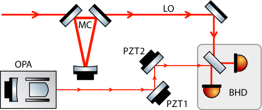
Refer to caption — Figure 1: Simplified sketch of the experimental setup. MC: spatial mode cleaner, LO: local oscillator, OPA: squeezed light source, BHD: balanced homodyne detector, PZT: piezo-electrically actuated mirror. PZT1 was used to control the average phase and PZT2 applied the phase noise.

The squeezed field propagated in free space from the OPA passing high-reflection mirrors, two of which were moved by piezo-electric transducers (PZT). One (PZT1, Fig. 1) was used to control the average phase of the squeezed field. The other (PZT2, Fig. 1) was driven by a quasi-random voltage to apply the phase diffusion. This voltage was generated by a high quality PC sound card connected to an appropriate amplifier. The sound card played back a previously generated sound file which was carefully designed to meet the desired shape of its frequency spectrum and its histogram. The former covered the flat part of the frequency response of the PZT but the frequency band of any control loop, the latter was chosen to be Gaussian for the partial phase diffusion and had to be absolutely flat in the totally randomized case.

Balanced homodyne detection (BHD) was used to measure the quadrature amplitude of the phase-diffused squeezed field. The visibility of the squeezed beam and the spatially filtered (MC, Fig. 1) local oscillator was 98.9% and was limited by OPA crystal inhomogeneities. The average quadrature phase of the BHD was servo loop controlled except for the total phase randomization where no mean phase exists. The signals of the two individual BHD-photodetectors were electronically mixed down at 7 MHz and low pass filtered with a bandwidth of 400 kHz to address a modulation mode showing good squeezing and a high dark noise clearance of the order of 20 dB. The resulting signals were fed into a PC based data acquisition system and sampled with one million samples per second and 14 bit resolution. For a more detailed description of the main parts of the setup we refer to [7, 6].

III Nonclassicality in terms of the characteristic function

III.1 Experimental demonstration

First, let us consider a sufficient criterion proposed in [8]: A state is nonclassical if the characteristic function $\Phi(\beta)$ of the $P$ function exceeds the characteristic function of the vacuum at some point $\beta$ :

\exists\beta:\quad|\Phi(\beta)|>|\Phi_{\rm vac}|\equiv 1.

(9)

Note that this condition represents the lowest order of a hierarchy of conditions which completely characterize the nonclassicality [12]. The function $\Phi(\beta)$ can be obtained by [13]

\Phi(\beta)=\left<:\hat{D}(\beta):\right>=\left<e^{i|\beta|\hat{x}(\pi/2-\arg(\beta))}\right>e^{|\beta|^{2}/2},

(10)

where $\hat{D}(\beta)$ is the displacement operator. Since we only consider a single quadrature, we may neglect the arguments of $\beta$ and $\hat{x}$ . The expectation value on the right hand side of Eq. (10) represents the characteristic function of the quadrature. It can be estimated from the sample of $N$ measured quadrature values $\left\{x_{j}\right\}_{j=1}^{N}$ via (cf. [14])

\left<e^{i|\beta|\hat{x}}\right>\approx\frac{1}{N}\sum_{j=1}^{N}e^{i|\beta|x_{j}}.

(11)

Inserting Eq. (11) into (10), we obtain an estimation $\overline{\Phi}(\beta)$ of ${\Phi}(\beta)$ . The variance of this quantity can be estimated as

\sigma^{2}\left\{\overline{\Phi}(\beta)\right\}=\frac{1}{N}\left[e^{|\beta|^{2}}-\left|\overline{\Phi}(\beta)\right|^{2}\right].

(12)

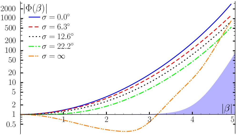
For each state we have recorded $N=10^{7}$ data points. The resulting characteristic functions are shown in Fig. 2. We only concentrate on the quadrature where the variance of the state is minimum. The shaded area corresponds to the magnitude of one standard deviation, it is added to the nonclassicality border $|\Phi_{\rm vac}(\beta)|\equiv 1$ . In order to demonstrate that a state satisfies the nonclassicality criterion, Eq. (9), with a significance of $s$ standard deviations, we have to check if the characteristic function satisfies the inequality

|\overline{\Phi}(\beta)|>1+s\sigma\left\{\overline{\Phi}(\beta)\right\}

(13)

at least at one point $\beta$ . It is clearly seen that all recorded states satisfy this lowest-order condition for nonclassicality with a high significance of $s\geq 10$ . Hence, we directly observe signatures of nonclassicality in the characteristic functions.

We note that Fig. 2 reveals that the $P$ functions of these states are highly singular. This is due to the fact that condition (9) is satisfied for all $\beta$ with large modulus, indicating that $\Phi(\beta)$ is not integrable. Therefore, we cannot expect $P(\alpha)$ to be a well-behaved function. However, if $\Phi(\beta)$ does not satisfy Eq. (9), one may be able to compute its Fourier transform and check nonclassicality of the state based on the failure of the $P$ function to be nonnegative, see [5].

III.2 Theoretical generalization of the results

Whereas in the experiment only states with Gaussian phase noise are investigated, we now prove that phase-diffused squeezed vacuum states always fulfill condition (9), indifferent of the phase distribution $p(\varphi)$ . Although this criterion is not necessarily fulfilled by an arbitrary nonclassical state, it turns out to be sufficient for any state with a characteristic function of the form (7).

First, we note that $\Phi_{\rm sv}(\beta;\varphi)$ is $\pi$ -periodic in the angle $\varphi$ . Without any loss of generality, we can assume that the function $p(\varphi)$ in Eq. (7) can be regarded as a probability density over the interval $[0,\pi]$ , i.e. $p(\varphi)\geq 0$ and $\int_{0}^{\pi}p(\varphi)d\varphi=1$ . For technical reasons, we may further assume that $p(\varphi)$ is $\pi$ -periodic as the characteristic function of squeezed vacuum, such that the domain of integration in Eq. (7) may be any interval of length $\pi$ .

It is clear that the average value of the function $p(\varphi)$ equals to ${\pi}^{-1}$ on any interval of length $\pi$ . As an intermediate result, we show that for any positive integer $n$ there exists an interval $[\varphi_{0}-\tfrac{\pi}{2n},\varphi_{0}+\tfrac{\pi}{2n}]$ on which the average of $p(\varphi)$ is greater or equal than ${\pi}^{-1}$ :

\forall n\in\mathbb{N}\quad\exists\varphi_{0}\in\mathbb{R}:\int_{-\frac{\pi}{2n}}^{\frac{\pi}{2n}}p(\varphi+\varphi_{0})d\varphi\geq\frac{1}{\pi}\frac{\pi}{n}=\frac{1}{n}.

(14)

Let us assume that this claim is wrong. Then we can find a certain $n$ such that

\forall\varphi_{0}\in\mathbb{R}:\qquad\int_{-\frac{\pi}{2n}}^{\frac{\pi}{2n}}p(\varphi+\varphi_{0})d\varphi<\frac{1}{n}

(15)

holds true. With this assumption we can decompose the interval $[0,\pi]$ into a set of $n$ successive intervals of the length $\frac{\pi}{n}$ and calculate

\int_{0}^{\pi}p(\varphi)d\varphi=\sum_{j=1}^{n}\int_{-\frac{\pi}{2n}}^{\frac{\pi}{2n}}p\left(\varphi+(j-\tfrac{1}{2})\tfrac{\pi}{n}\right)d\varphi<\sum_{j=1}^{n}\frac{1}{n}=1,

(16)

which is in clear contradiction to the normalization condition of $p(\varphi)$ . Consequently, our assumption is wrong, and the desired statement is verified.

Now let us look at the characteristic function defined in Eqs. (6) and (7). We assume that the $x$ -quadrature is the squeezed one, so $V_{x}<1<V_{p}$ . Hence, we can find a positive integer $n$ such that

\forall\varphi\in[-\tfrac{\pi}{2n},\tfrac{\pi}{2n}]:\quad 1-V_{x}\cos^{2}(\varphi)-V_{p}\sin^{2}(\varphi)>0

(17)

holds. Simultaneously, we can find a real number $\varphi_{0}$ such that the inequality (14) is fulfilled, and choose $\beta=|\beta|e^{i\varphi_{0}}$ . Making use of the simple relations

\Phi_{\rm sv}(\beta;\varphi)=\Phi_{\rm sv}(\beta e^{-i\varphi};0),\quad\Phi_{\rm sv}(\beta;0)=\Phi_{\rm sv}(\beta^{*};0),

(18)

and taking into consideration that the domain of integration in Eq. (7) may be an arbitrary interval of length $\pi$ , we calculate

$\displaystyle\Phi(\|\beta\|e^{i\varphi_{0}})$	$\displaystyle=$	$\displaystyle\int_{\varphi_{0}-\tfrac{\pi}{2}}^{\varphi_{0}+\tfrac{\pi}{2}}p(\varphi)\Phi_{\rm sv}(\|\beta\|e^{i\varphi_{0}};\varphi)\,d\varphi$	(19)
	$\displaystyle=$	$\displaystyle\int_{\varphi_{0}-\tfrac{\pi}{2}}^{\varphi_{0}+\tfrac{\pi}{2}}p(\varphi)\Phi_{\rm sv}(\|\beta\|e^{i(\varphi_{0}-\varphi)};0)\,d\varphi$
	$\displaystyle=$	$\displaystyle\int_{-\tfrac{\pi}{2}}^{\tfrac{\pi}{2}}p(\varphi+\varphi_{0})\Phi_{\rm sv}(\|\beta\|e^{i\varphi};0)\,d\varphi.$

Since the integrand is nonnegative, a diminution of the domain of integration decreases the value of the integral:

\left|\Phi(|\beta|e^{i\varphi_{0}})\right|\geq\int_{-\tfrac{\pi}{2n}}^{\tfrac{\pi}{2n}}p(\varphi+\varphi_{0})\Phi_{\rm sv}(|\beta|e^{i\varphi};0)\,d\varphi.

(20)

Because $n$ is chosen such that Eq. (17) is fulfilled for each $\varphi$ in the domain of integration, there exists an $\epsilon>0$ such that

\forall\varphi\in[-\tfrac{\pi}{2n},\tfrac{\pi}{2n}]:\quad\left|\Phi_{\rm sv}(|\beta|e^{i\varphi})\right|\geq e^{\epsilon|\beta|^{2}/2}.

(21)

Consequently, we have a lower bound for Eq. (20):

\displaystyle|\Phi(|\beta|e^{i\varphi_{0}};0)|

\displaystyle\geq

\displaystyle e^{\epsilon|\beta|^{2}/2}\int_{-\tfrac{\pi}{2n}}^{\tfrac{\pi}{2n}}p(\varphi+\varphi_{0})\,d\varphi

(22)

Additionally, we have chosen $\varphi_{0}$ such that Eq. (14) is fulfilled. Therefore,

|\Phi(|\beta|e^{i\varphi_{0}})|\geq\frac{e^{\epsilon|\beta|^{2}/2}}{n}.

(23)

Obviously, the characteristic function $\Phi(\beta)$ is not bounded, independently of the phase noise distribution $p(\varphi)$ . Consequently, we are always able to prove nonclassicality by means of Eq. (9), which is the most simple criterion among a necessary and sufficient hierarchy [12].

IV Nonclassicality in terms of moments

Besides the signatures of nonclassicality in terms of the characteristic function, different criteria for demonstrating nonclassicality are known. Since we measured time series of individual quadrature values we can calculate all higher-order moments of the quadrature operator $\hat{x}$ .

IV.1 Hong-Mandel squeezing

We begin by examining higher-order squeezing as proposed by Hong and Mandel [9]. To this end, we calculate the degree of $2n$ -th order squeezing

q_{2n}=\frac{\left<(\Delta\hat{x})^{2n}\right>}{(2n-1)!!}-1,\qquad n\in\mathbb{N}

(24)

where $\Delta\hat{x}=\hat{x}-\left<\hat{x}\right>$ . The moments can be estimated from the sample of quadrature data quite naturally by replacing expectation values by their arithmetic means. It is sufficient to verify nonclassicality if at least one of the $q_{2n}$ is negative.

$\sigma/{}^{\circ}$	$q_{2}$	$q_{4}$	$q_{6}$	$q_{8}$	$q_{10}$
$0.0$	$-0.6362(1\pm 0.3\%)$	$-0.8667(1\pm 0.16\%)$	$-0.9506(1\pm 0.12\%)$	$-0.9813(1\pm 0.09\%)$	$-0.9927(1\pm 0.07\%)$
$6.3$	$-0.5717(1\pm 0.04\%)$	$-0.8090(1\pm 0.03\%)$	$-0.9102(1\pm 0.03\%)$	$-0.9549(1\pm 0.04\%)$	$-0.9754(1\pm 0.06\%)$
$12.6$	$-0.4060(1\pm 0.08\%)$	$-0.5509(1\pm 0.15\%)$	$-0.5459(1\pm 0.60\%)$	$-0.3852(1\pm 4.2\%)$	$0.0798(1\pm 95\%)$
$22.2$	$0.0196(1\pm 3.2\%)$	$0.6864(1\pm 0.53\%)$	$2.982(1\pm 0.84\%)$	$10.61(1\pm 1.7\%)$	$37.27(1\pm 3.3\%)$
$\infty$	$1.908(1\pm 0.09\%)$	$10.68(1\pm 0.16\%)$	$51.72(1\pm 0.32\%)$	$249.6(1\pm 0.65\%)$	$1222(1\pm 1.23\%)$

Table 2: Degree of squeezing

q_{2n}

for different orders

2n

and standard deviations of phase noise

\sigma

Table 2 shows the degree of squeezing for different orders and different phase noise strengths. Obviously, only if the lowest-order parameter $q_{2}$ is negative, then the parameter $q_{2n}$ of higher order can also be negative. Hence, we may only observe higher-order squeezing if the state already shows standard squeezing. The investigation of the degree of higher-order squeezing does not extend the range of detection of nonclassicality of phase-diffused squeezed states. This is not surprising, since it can be shown that for Gaussian states (3) the degree of squeezing is given by

q_{2n}(\varphi)=\left[V_{x}\cos(\varphi)+V_{p}\sin(\varphi)\right]^{n}-1.

(25)

For these states, squeezing always implies higher-order squeezing and vice versa [9]. Phase diffusion can only smooth out the phase dependence of the moments and diminish the nonclassical effect.

IV.2 Matrices of normally ordered moments

Normally ordered moments of the quadrature operator $\hat{x}$ can be estimated from measured data points $\{x_{j}\}_{j=1}^{N}$ via appropriate sampling relations (see Appendix A),

\left<:\hat{x}^{k}:\right>\approx\frac{1}{2^{k/2}N}\sum_{j=1}^{N}H_{k}\left(\tfrac{x_{j}}{\sqrt{2}}\right),

(26)

where $H_{k}(x)$ are the Hermite polynomials. With these moments at hand, we can examine the nonclassicality criterion of Agarwal [10]. It has been shown that a state is nonclassical if at least one of the matrices

M^{(l)}=\left(\begin{array}[]{c c c c}1&\left<:\hat{x}:\right>&\ldots&\left<:\hat{x}^{l-1}:\right>\\ \left<:\hat{x}:\right>&\left<:\hat{x}^{2}:\right>&\ldots&\left<:\hat{x}^{l}:\right>\\ \vdots&\vdots&\ddots&\vdots\\ \left<:\hat{x}^{l-1}:\right>&\left<:\hat{x}^{l}:\right>&\ldots&\left<:\hat{x}^{2l-2}:\right>\\ \end{array}\right)

(27)

is not positive semidefinite. This can be verified by showing that at least one of the principal minors of such a matrix is negative [15]. However, to this end we had to check up to $2^{l}-1$ principal minors for each matrix $M^{(l)}$ , which is a computationally expensive task.

Here we use the fact that the existence of a negative eigenvalue of $M^{(l)}$ demonstrates the violation of positive semidefiniteness. Therefore, we determine

\lambda_{\rm min}^{(l)}=\min_{\vec{x}\neq\vec{0}}\frac{\vec{x}^{T}M^{(l)}\vec{x}}{\vec{x}^{T}\vec{x}}

(28)

via a conjugate gradient algorithm, see, e.g., [16]. It can be shown that $\lambda_{\rm min}^{(l)}$ equals to the minimum eigenvalue of $M^{(l)}$ . In this way, we only need to calculate one quantity per matrix to examine its definiteness. Its standard deviation is determined by using a bootstrap method: We generate new quadrature data, distributed as the experimentally measured quadratures, $100$ times to obtain a statistical sample of eigenvalues, which gives the standard deviation, cf. [17].

$\sigma/{}^{\circ}$	$2\times 2$ Matrix	$4\times 4$ Matrix	$6\times 6$ Matrix	$8\times 8$ Matrix	$10\times 10$ Matrix
$0.0$	$-0.6362(1\pm 0.25\%)$	$-4.294(1\pm 0.86\%)$	$-104.0(1\pm 2.5\%)$	$-6201(1\pm 6.1\%)$	$-722\cdot 10^{3}(1\pm 12\%)$
$6.3$	$-0.5717(1\pm 0.03\%)$	$-3.337(1\pm 0.11\%)$	$-69.93(1\pm 0.35\%)$	$-3593(1\pm 0.98\%)$	$-335\cdot 10^{3}(1\pm 2.5\%)$
$12.6$	$-0.4060(1\pm 0.08\%)$	$-2.040(1\pm 1.1\%)$	$-6.728(1\pm 53\%)$	$-107.4(1\pm 110\%)$	$-1259\cdot 10^{3}(1\pm 49\%)$
$22.2$	$0.0197(1\pm 3.0\%)$	$-0.2323(1\pm 1.1\%)$	$-0.5358(1\pm 4.1\%)$	$-2.299(1\pm 71\%)$	$-459\cdot 10^{3}(1\pm 40\%)$
$\infty$	$1.0000(1\pm 0\%)$	$0.7856(1\pm 1.2\%)$	$0.5493(1\pm 12\%)$	$10.85(1\pm 13\%)$	$1113(1\pm 94\%)$

Table 3: Table of minimum eigenvalues of the matrices

M^{(l)}

for different

l

and phase noise

\sigma

. The existence of significantly negative values indicate the nonclassicality.

The experimental results are shown in Table 3. We only consider matrices of even dimension, since we noted that the minimum eigenvalues of $M^{(2n)}$ and $M^{(2n+1)}$ are equal. This may be due to the fact that odd moments of squeezed vacuum states vanish, giving the matrices a special structure. We observe that all matrices, which belong to the states showing squeezing, have significantly negative eigenvalues. Hence, their nonclassical character can be directly observed in the sign of the smallest eigenvalue. Furthermore, for the states with $\sigma\geq 22.2^{\circ}$ the matrix $M^{(2)}$ is positive semidefinite, since this directly corresponds to the absence of quadrature squeezing. However, for the state with $\sigma=22.2^{\circ}$ the matrices $M^{(l)}$ with $l\geq 4$ possess a negative eigenvalue. Therefore, Agarwal’s criterion extends the range of detection of nonclassicality. Only for the completely phase-diffused state, are we not able to prove nonclassicality by this method. For this state, the effect might appear in higher-dimensional matrices, but the statistical uncertainty might hide the effect.

V Conclusion

We have used experimental data sets of quadrature measurements on phase-diffused squeezed states for a test of different nonclassicality criteria. Even for a completely phase-diffused squeezed state, i.e. where the measured statistics were identical for all homodyne detection phase angles, we found a pronounced nonclassical character. This could be illustrated with the help of the characteristic function of the $P$ function: It directly shows nonclassical features in the lowest-order criterion of [12] and the nonclassicality was detected with a rather high signal-to-noise ratio. Other nonclassicality criteria, such as higher-order squeezing or the violation of positive semidefiniteness of Agarwal’s matrices, fail to reveal nonclassicality beyond squeezing or only show nonclassical behavior in matrices of higher dimension. Therefore, we demonstrated for the radiation under study, that the characteristic function of the $P$ function, which contains information about all moments of the state, can be a more powerful tool for the examination of nonclassicality than a finite set of moments.

Eventually, we note that the evaluation of the statistical significance of nonclassical effects is much easier in terms of characteristic functions, since Eq. (12) provides a simple relation between the variance and the value of $\Phi(\beta)$ . Testing the definiteness of matrices of moments requires complex nonlinear procedures, for instance the calculation of the smallest eigenvalue or the principal minors. This leads to complications in the estimation of the statistical significance, which increase the computational effort. For matrices of high orders the resulting errors are large and they may hide the sought nonclassical effects.

Acknowledgements

We thank J. Fiurášek for many helpful discussions.

Appendix A Sampling formula for normally ordered moments

The characteristic function $\Phi(\beta)$ can be given in terms of normally ordered moments of the creation and annihilation operator [13]:

\displaystyle\Phi(\beta)

\displaystyle=

\displaystyle\sum_{k=0}^{\infty}\frac{1}{k!}\left<:\left(\beta\hat{a}^{\dagger}-\beta^{*}\hat{a}\right)^{k}:\right>.

(29)

Introducing the phase-dependent quadrature operator $\hat{x}(\varphi)=\hat{a}^{\dagger}e^{-i\varphi}+\hat{a}e^{i\varphi}$ , we have

\Phi(\beta)=\sum_{k=0}^{\infty}\frac{(i|\beta|)^{k}}{k!}\left<:\hat{x}(\tfrac{\pi}{2}-\arg(\beta))^{k}:\right>.

(30)

Consequently, the normally ordered moments $\left<:\hat{x}(\varphi)^{k}:\right>$ can be calculated from the characteristic function of the $P$ function as

\left<:\hat{x}(\varphi)^{k}:\right>=\frac{\partial^{k}}{\partial(ib)^{k}}\Phi(ibe^{-i\varphi})\bigg|_{b=0}.

(31)

To obtain a formula which can be applied in practice, we insert Eq. (10) into Eq. (31) and use the definition of the Hermite polynomials in the form $(-1)^{k}H_{k}(\xi)e^{-\xi^{2}}=\frac{\partial^{k}}{\partial\xi^{k}}e^{-\xi^{2}}$ with $\xi=ib/\sqrt{2}$ . Neglecting the phase argument, we find

$\displaystyle\left<:\hat{x}^{k}:\right>$	$\displaystyle=$	$\displaystyle\frac{\partial^{k}}{\partial(ib)^{k}}\left<e^{ib\hat{x}}\right>e^{b^{2}/2}\bigg\|_{b=0}$	(32)
	$\displaystyle=$	$\displaystyle\left<\frac{\partial^{k}}{\partial(\sqrt{2}\xi)^{k}}e^{-\left[\xi-\hat{x}/\sqrt{2}\right]^{2}}e^{\hat{x}^{2}/2}\right>\bigg\|_{\xi=0}$
	$\displaystyle=$	$\displaystyle\left<\frac{(-1)^{k}}{2^{k/2}}H_{k}\left(\xi-\tfrac{\hat{x}}{\sqrt{2}}\right)e^{-\left[\xi-\tfrac{\hat{x}}{\sqrt{2}}\right]^{2}}e^{\tfrac{\hat{x}^{2}}{2}}\right>\bigg\|_{\xi=0}$
	$\displaystyle=$	$\displaystyle\frac{1}{2^{k/2}}\left<H_{k}\left(\tfrac{\hat{x}}{\sqrt{2}}\right)\right>.$

Hence, we obtain normally ordered moments from measured quadratures via

\left<:\hat{x}^{k}:\right>\approx\frac{1}{2^{k/2}N}\sum_{j=1}^{N}H_{k}\left(\tfrac{x_{j}}{\sqrt{2}}\right),

(33)

The approximation sign indicates that the right hand side is a statistical estimator.

References

[1] E. Schrödinger, Naturwiss. 14, 664 (1926).
[2] E. C. G. Sudarshan, Phys. Rev. Lett. 10, 227 (1963).
[3] R. J. Glauber, Phys. Rev. 131, 2766 (1963).
[4] U. M. Titulaer and R. J. Glauber, Phys. Rev. 140, B676 (1965).
[5] T. Kiesel, W. Vogel, V. Parigi, A. Zavatta and M. Bellini, Phys. Rev. A 78, 021804(R) (2008).
[6] A. Franzen, B. Hage, J. DiGuglielmo, J. Fiurášek and R. Schnabel, Phys. Rev. Lett. 97, 150505 (2006).
[7] B. Hage, A. Franzen, J. DiGuglielmo, P. Marek, J. Fiurášek and R. Schnabel, New J. Phys. 9 227 (2007).
[8] W. Vogel, Phys. Rev. Lett. 84, 1849 (2000).
[9] C. K. Hong and L. Mandel, Phys. Rev. Lett. 54, 323 (1985).
[10] G. S. Agarwal, Opt. Commun. 95, 109 (1993).
[11] J. Fiurášek, P. Marek, R. Filip, and R. Schnabel, Phys. Rev. A 75, 050302(R) (2007).
[12] T. Richter and W. Vogel, Phys. Rev. Lett. 89, 283601 (2002).
[13] W. Vogel and D.-G. Welsch, Quantum Optics, (Wiley-VCH, Weinheim, 2006).
[14] A. I. Lvovsky and J. H. Shapiro, Phys. Rev. A 65, 033830 (2002).
[15] E. V. Shchukin, W. Vogel, Phys. Rev. A 72, 043808 (2005).
[16] X. Yang, T. K. Sarkar, E. Arvas, IEEE Trans. Acoust., Speech, Signal Processing 37, 1550 (1989).
[17] J. Shao and D. Tu, The Jackknife and Bootstrap, (Springer, New York, 1995).