Matched asymptotic expansions
for twisted elastic knots:
a self-contact problem with non-trivial contact topology
Abstract
We derive solutions of the Kirchhoff equations for a knot tied on an infinitely long elastic rod subjected to combined tension and twist. We consider the case of simple (trefoil) and double (cinquefoil) knots; other knot topologies can be investigated similarly. The rod model is based on Hookean elasticity but is geometrically non-linear. The problem is formulated as a non-linear self-contact problem with unknown contact regions. It is solved by means of matched asymptotic expansions in the limit of a loose knot. Without any a priori assumption, we derive the topology of the contact set, which consists of an interval of contact flanked by two isolated points of contacts. We study the influence of the applied twist on the equilibrium.
1 Introduction
Knots are found in everyday life, shoe lacing being probably the most common example. They are also essential in a number of activities such as climbing and sailing. In science, knots have long been studied in the field of mathematics, the main motivation being to propose a topological classification of the various knot types, see the review by Tabor and Klapper (1994). Recently, there has been an upsurge of interest in knots in the biological context: knots form spontaneously in many long polymers chains such as DNA (Katritch et al., 1996) or proteins, and have been tied on biological filaments (Arai et al., 1999). Knotted filaments have a lower resistance to tension than unknotted ones and break preferably at the knot (Saitta et al., 1999; Pieranski et al., 2001a). Despite a wide range of potential applications, the mechanics of knots is little advanced. The present paper is an attempt to approach knots from a mechanical perspective by using a well-established model of thin elastic rods.
The problem of finding so-called ideal knot shapes has received much attention in the past decade (Katritch et al., 1996; Stasiak et al., 1998). In this geometrical description of tight knots, a impenetrable tube with constant radius is drawn around an inextensible curve in Euclidean space and one seeks, for each knot type, the configurations of the curve such that the radius of the tube is maximum. The case of open knots, where the curve does not close upon itself, has been studied by Pieranski et al. (2001b) in connection with the breakage of knotted filaments under tension (Pieranski et al., 2001a).
To go beyond a purely geometrical description of knots, it is natural to formulate the problem in the framework of the theory of elasticity. The case of tight knots, or even of moderately tight knots, leads to a problem of 3D elasticity with geometrical nonlinearities (finite rotations), finite strains, and self-contact along an unknown surface: there is no hope to derive analytical solutions. Numerical solution of this problem raises considerable difficulties too, which have not yet been tackled to the best of our knowledge. In the present paper, we study the limit of loose knots, when the total contour length captured in the knot is much larger than the radius of the filament. In this limit, it is possible to use a Cosserat type model and describe the rod as an inextensible curve embedded with a material frame, obeying Kirchhoff equations; as we show, the equilibria of open knots can be solved analytically in this limit.
Self-contact in continuum mechanics, and in the theory of elastic rods in particular, leads to problems that are both interesting and difficult. This comes from the fact that the set of points in contact is not known in advance — in fact, not even the topology of this set is known. This paper builds up on prior work by von der Mosel (1999); Schuricht and von der Mosel (2003), who characterizes the smoothness of the contact force in equilibria of elastic rods, and by Coleman and Swigon (2000), who write down the Kirchhoff equations for rods in self-contact explicitly, including the unknown contact force. These equations have been solved by numerical continuation in specific geometries by Coleman and Swigon (2000); van der Heijden et al. (2003); Neukirch (2004). In these papers, the authors simultaneously solve for the non-linear Kirchhoff equations and for the unknown contact forces. In the present paper, we shown that, under the same set of assumptions that warrant applicability of the Kirchhoff equations, one can in fact neglect the geometrical nonlinearities in the region of self-contact. As a result, nonlinearities and contact can be addressed in well separated spatial domains. This brings in an important simplification and, as the result, we are able for the first time to derive analytical solutions of a self-contact problem for rods undergoing finite displacement, exhibiting a non-trivial contact set topology.
Our solution is constructed with matched asymptotic expansions with respect to a small parameter which is zero for a perfectly thin rod. As is done routinely in boundary layer analysis, we use qualitative reasonings (dimensional analysis) to justify how the various quantities scale with the small parameter . We emphasize that our final solution is exact and does not involve any other assumption than the smallness of the parameter : it is asymptotically exact. Our presentation is based on formal expansions; proofs of convergence are beyond the scope of the present paper and can hopefully be established in the future.
In the present paper, we consider a knot loaded under mixed tension and twist . In a previous short paper (Audoly et al., 2007), we have announced some of the results reported here, for the case of a purely tensile loading, . In addition to presenting a justification of these results, we address here the influence of twist on the knot shape.
The outline of the present paper is as follows. In Section 2, we introduce the Kirchhoff equations for rods in equilibrium, including the contact forces relevant for the knotted geometry; we discuss the equivalent formulation as a minimization problem with topological constraints. In Section 3, we consider the case of an elastic curve with vanishing thickness and show that the region of contact collapses to a point connecting a circular loop and two straight tails. In Section 4, we carry out the dimensional analysis of the solution with small but nonzero thickness. We show that the equilibrium solution is composed of three types of regions, namely a loop and two tails connected by a braid. The scaling of the unknowns with the small dimensionless parameter are identified. Following the general methodology of matched asymptotic expansion, we use these scalings to devise a perturbation scheme of the original equations in (non-integer) powers of . The resulting equations are written down and solved in the various regions: the tails are solved in Section 5, the loop in Section 6. The solution in the braid region is the most challenging as this is where contact occurs, and in Section 7 we obtain a universal solution describing the shape of the rod in this region. In Section 8 we build a global solution by matching the solutions derived previously in each region. We obtain a unique equilibrium solution for any given value of the loading parameters (force and twist). In Section 9, this theory is validated by experiments. Appendix A discusses the topology of the contact set in more details.
2 Model
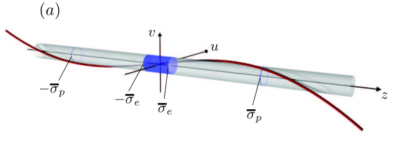
We seek equilibrium solutions of a thin elastic rod bent into an open 11 1 In topology, a knot is defined as a closed, non self-intersecting curve. Here we consider curves having two infinite tails, hence the name ‘open knots’. knot with a prescribed type, and subjected to tensile end force and torsional end moment, as shown on Fig. 2. In the present paper, we focus on two specific knot types, which are open trefoil knots, also called simple knot and noted , and open cinquefoil knots, also called double knot and noted , see Fig. 1.
Other knot types can be handled similarly. The rod is infinitely long and the loading is applied at infinity.
Our model is based on the Kirchhoff equations for the mechanical equilibrium of elastic rods. We consider the case of an unshearable 22 2 By unshearable, we mean that the rod satisfies the Navier-Bernoulli kinematical hypothesis. , inextensible rod with circular cross-section --- this is the standard model for elastic rods, which can be derived under fairly general hypotheses from 3D elasticity theory 33 3 Extensions of the present results to different rod models do not raise any fundamental difficulty.. Contact of the rod with itself is assumed to be frictionless. The mathematical formulation of the problem is based on classical models and is relatively straightforward; the challenge of the present analysis is to deal with geometrical nonlinearities and self-contact — one of our contributions is to determine the topology of the contact set which is not known in advance.
In the present section, we recall the Kirchhoff equations for rods and show how they can be applied to the geometry considered. We emphasize the minimization problem underlying the equations of equilibrium, and put the equations in a dimensionless form.
2.1 Kinematics
We consider an infinite isotropic elastic rod, bent into an open knot as shown in Fig. 2, with a circular cross section of radius , a bending modulus and a twisting modulus . Centerline of the rod is parameterized by the arc-length and is defined by its Cartesian equation,
where the orientation of the axes is specified below. The tangent to the centerline is noted
| (1) |
Since the rod is assumed inextensible, the tangent is a unit vector,
| (2) |
for all . We note the internal moment in the rod and the internal force — these variables describe stress distribution in the cross-section in Kirchhoff theory of rods.
2.2 Constitutive relations
We assume a linear elastic response (Hookean elasticity), which is consistent with the small strain approximation underlying Kirchhoff theory. The constitutive law for a rod with symmetric (e. g. circular) cross-section can be conveniently written in vector form (Landau and Lifshitz, 1981):
| (3) |
where is the material twist of the rod. The above expression is a condensed form of the constitutive relations for a rod that are usually written in coordinates in the material frame. The first term in the right-hand side is the bending moment and lies in the cross-section; for a symmetric rod, this bending moment is the binormal, , times the bending stiffness . The second term in the right-hand side is the twisting moment and is along the tangent: the twisting moment is the material twist, , times the twist stiffness . Since the rod is considered inextensible and unshearable, the internal force is the Lagrange multiplier associated with these kinematical constraints, and it not given by a constitutive law.
2.3 Loading
At the end of the rod corresponding to , a tensile force and a torsional moment are applied, see Fig. 2. These two vectors are assumed to be collinear, and are used to define the axis . Global mechanical equilibrium requires that an opposite force and moment are applied at the other end, . At equilibrium, the two long tails of the rod will be aligned with the direction of the force. Owing to our choice of axis, we write
Stability of the long tails require but the twist can be positive or negative.
2.4 Symmetry
Given the symmetry of the loading, we focus 44 4 Since the equations are non-linear, one could argue that some solutions having no symmetry at all could exist, as happens in buckling problems. We would miss such solutions since we restrict the analysis to the symmetric case from the beginning. This remark applies to the case of a finite thickness , but to the problem addressed here, which concerns the limit of a small thickness . In this limit, we show that the equations can be linearized; using the principle of linear superposition, one can focus on symmetric solutions. on equilibrium solutions that are symmetric. More accurately, we assume that the knotted rod is invariant by rotation with angle about an axis perpendicular to the axis defined by the loading. This is consistent as the endpoints at infinity are swapped by this transformation, and so the loading is globally invariant under this transformation 55 5 Note that the knot is not invariant by a reflection with respect to a plane perpendicular to the axis: this reflection leaves the loading globally invariant but changes the knot type, turning a left-handed knot into a right-handed one..
Let us call the axis defining this symmetry by rotation with an angle . The intersection of the perpendicular axes and defined so far will be the origin of our Cartesian coordinates. The direction perpendicular to and defines the third axis , in such a way that is direct and orthonormal. Intersection of the axis of symmetry with the centerline defines what can be called the midpoint of the rod — intuitively, this is the bottom of the loop in Fig. 2. This midpoint is taken as the origin of the arc-length coordinate, . With this convention, the symmetry by rotation about with angle maps a point on the centerline with coordinate onto the point with opposite coordinate . Using this property, it is sufficient to find the equilibrium shape of the rod over one half, say the positive half : the other half can be found by applying the symmetry.
2.5 Variational formulation, constraints
The equilibrium shape of the knotted rod can be found be solving a minimization problem: this equilibrium shape is a minimizer of the total energy of the rod (potential energy associated with loading at endpoints plus elastic energy) under the combined constraints of inextensibility, non-penetration and prescribed knot topology. This variational view of the problem will be useful later for solving the braid region in Section 7.
The total energy of the rod is defined as:
| (4) |
where and stand for the curvature and the twist of the rod. The integral term in the right-hand side is the elastic energy associated with the constitutive law (3). The bending term depends on the scalar curvature
| (5) |
The last two terms in equation (4) represent the work of the applied tensile force , related to the end-to-end shortening , and of the applied torsional moment , related to the relative rotation of the ends.
The minimization of this energy is subjected to a series of constraints. First, the inextensibility constraint is expressed by equation (2). Second, the topology of the knot is prescribed (this topological constraint cannot be written down easily in the general case; it will be shown to impose the value of a winding index in the braid when we focus on loose knots later on). Third and lastly, one has to consider the non-penetration constraint which can be expressed as:
| (6) |
for any and such that . Note that the radius of the rod enters in the equation at this point in the right-hand side of equation (6). The trick of restricting the penetration test to couples of points separated by a curvilinear distance greater than is due to von der Mosel (1999), and avoids mistaking close neighbors on the centerline for points violating the non-penetration condition — it is given for mathematical consistency but is not needed in the following: for the problem we consider, we know a priori that the arc-length separation of two points in contacts is large, namely of order where the radius of the loop is a known quantity of order 1.
2.6 Equilibrium: Kirchhoff equations
The equilibrium equations for a rod can be derived from the energy (4) by the Euler-Lagrange method (Bourgat et al., 1988; Steigmann and Faulkner, 1993). This leads to the following equations:
| (7a) | |||
| (7b) | |||
| (7c) | |||
| (7d) | |||
where primes denote derivation with respect to arc-length . The first equation is the definition of the tangent, already encountered in equation (1). The second equation combines the constitutive relations (3) with the definition (5) of curvature. The last two equations express the equilibrium of moments and forces on an infinitesimal rod element, and are known as the Kirchhoff equations (Landau and Lifshitz, 1981). The vector is the density of distributed force per unit length applied on the rod, sometimes referred to as the contact pressure. In the present problem, gravity is neglected and the only force to be considered is the one arising from the contact pressure in the regions of contact — if there is no contact, .
2.7 Contact set, contact force
Let us define the contact set as the set of couples of arc-lengths, , defining cross-sections that are in contact:
| (8) |
where the first inequality, , is to avoid mistaking close neighbors for regions of penetrations, as explained earlier, and the second inequality is the contact criterion.
We are touching here the main challenge of self-contact problems: the profile of the contact pressure is required to compute the centerline by integration of the Kirchhoff equations, but it depends itself non-linearly on the geometry of contact, that is on the shape of the centerline. In other words, and the contact set must be determined in a self-consistent way but none is known a priori. In particular, the topology of the contact set is not known in advance. It will be obtained later as an outcome of our calculations.
For any couple in the set , the corresponding cross-section are in contact. By the action-reaction principle, we have . In addition we assume frictionless contact: the force has to be normal to the rod surface, and so is aligned with . This implies that the contact force is aligned with the vector joining the points and :
| (9) |
for . In this equation we have introduced the scalar contact pressure ; since the rod is a 1D object, the contact force has the dimension of a force per unit length but we shall nevertheless call it a contact pressure. For the solution to be physical, the pressure must be positive:
| (10) |
In terms of the scalar contact pressure, the action-reaction principle can be rewritten as
| (11) |
2.8 Boundary conditions
Thanks to the symmetry introduced in Section 2.4, the equations of equilibrium (7) need be solved over half the rod only, that is for . These equations form a boundary value problem as there are conditions to be satisfied at both ends of the interval. The following conditions must be satisfied at the endpoint :
| (12a) | |||
| (12b) | |||
| (12c) | |||
| (12d) | |||
The asymptotic conditions holding at the opposite end of the rod, , can be found by symmetry. The first two asymptotic conditions above enforce the loading applied at infinity. Condition (12c) imposes that the tangent is asymptotically aligned with the applied force, which is an obvious necessary condition for minimizing the energy. The last condition (12d) defines the axis as the asymptote of the centerline far away from the knot — without this convention there would be infinitely many solutions, corresponding to the invariance of the system under rigid-body translations perpendicular to the axis.
The boundary conditions at the midpoint of the rod derive from the invariance of the solution by a rotation of angle about the axis:
| (13a) | ||||
| (13b) | ||||
| (13c) | ||||
| (13d) | ||||
The justification for each of these three equations is similar, and will be given here for the first one only. Let us write the Cartesian coordinates of the tangent at midpoint as . According to our symmetry assumption, rotating the system by an angle about the axis is equivalent to reversing the orientation of the centerline. The first operation changes the tangent to , while the second one changes it to its opposite, . Equality of these two vectors imposes , which yields equation (13a).
2.9 Invariants
Due to their variational nature, the equilibrium equations (7) are associated with several invariants as discussed by Maddocks and Dichmann (1994). These invariants are known to be conserved in the absence of distributed force, . In the present case, the distributed force can be nonzero but remains everywhere perpendicular to the tangent . Under this assumption, it is straightforward to check that the following expressions are still invariants:
| (14) |
The first invariant is directly proportional to the material twist , and is known to be uniform for a rod with symmetric cross-section in equilibrium in the absence of distributed torques. The famous Kirchhoff analogy identifies the equations of equilibrium of a symmetric rods to the equations of motion of a table top subjected to gravity. According to this analogy, the first invariant expresses conservation of the angular moment about the axis of the top; the second invariant expresses conservation of the energy of the top.
The constant values of these invariants are imposed by the boundary conditions (12):
| (15a) | |||
| and | |||
| (15b) | |||
Note that conservation of these invariants requires frictionless contact.
2.10 Dimensionless form
The problem has been formulated so far in terms of the loading parameters and , of the thickness , and of the elastic stiffnesses and . In this section, we use dimensional analysis and rewrite the equations in a form that depends on two dimensionless parameters, and , only.
To this end, we introduce the characteristic length , force and moment as follows:
| (16) |
These quantities are used to define dimensionless variables, noted with a bar. For instance, we define the dimensionless arc-length and position as
| (17) |
Note that rescaled functions, such as , are always considered to be a function of a rescaled argument, here and not : a prime on a barred function implies that derivation is with respect to the rescaled arc-length. For instance, the rescaled tangent is defined by
and happens to be the same unit vector as the physical tangent , evaluated at the corresponding point . Similarly, the rescaled curvature is defined as :
| (18) |
The rescaled internal moment and torsional couple are:
| (19) |
The internal force is naturally rescaled using the typical force , while the contact force per unit length, , is rescaled using the dimension :
| (20) |
Having defined the rescaled form of the various quantities, we proceed to rewrite the equations of the problem in dimensionless form. We start with the constitutive relation (3):
| (21) |
The kinematical relations and equilibrium equations (7) write:
| (22a) | |||
| (22b) | |||
| (22c) | |||
| (22d) | |||
For the asymptotic conditions (12) we obtain:
| (23a) | |||
| (23b) | |||
| (23c) | |||
| (23d) | |||
while the midpoint conditions take the same form as the original expressions (13), with original variables replaced by barred ones:
| (24a) | ||||
| (24b) | ||||
| (24c) | ||||
| (24d) | ||||
In rescaled form, the invariants (15) read:
| (25a) | ||||
| (25b) | ||||
We now turn to the non-penetration constraint. In terms of , Eq. (6) can be rewritten as
In the right-hand side a fundamental dimensionless number of the problem has appeared, namely the ratio of the rod thickness to the characteristic length built from the traction force and the bending stiffness of the rod. It will be convenient to deal with this dimensionless number using an auxiliary number defined as
| (26) |
This details of the present definition of will be motivated later in Eq. (31). In terms of , the non-penetration condition can be written as
| (27) |
In equations (21) to (27), we have rewritten all the equations of the problem in terms of two dimensionless parameters only, and , defined in Eqs. (19) and (26) respectively. The first parameter is the rescaled torsional moment; the second parameter is the aspect-ratio of the rod. In this paper, we focus on the limit of thin rod, or a loose knot, , and build an asymptotic solution of the set of equations above, for arbitrary values of .
3 Zero radius solution
Before we build a solution of the equations for small , it is useful to consider the limit of an infinitely thin rod, , that is the problem of tying a knot on an elastic curve. This case corresponds to , and is the subject of the present section.
As we shall show later, the limit is singular: the contact region has nonzero length for but shrinks to a point in the limit . It follows that the solution of the limit problem () is less regular than the solutions for and must be defined in a weak sense. In addition, the topological constraint on the knot type is not easy to write down for the limit problem. We shall not study convergence for in a mathematically rigorous way. Following a pragmatic approach, a solution for is constructed in the present Section based on some assumptions (planarity, existence of a point-like contact). These assumptions will be validated later when we show that it is possible to extend this solution into a family of smooth solutions indexed by .
3.1 Explicit solution
In the limit of zero thickness , we consider a solution made up of a circular loop connected to two straight, semi-infinite tails. Owing to the assumed symmetry of the solution, we focus on one half the rod and consider a half-circle starting from the midpoint, connected to a single straight, semi-infinite tail. There is no contact, except at the singular point where the loop and tail merge, see Fig. 3. By our previous definition of axes, this point is the origin of the Cartesian frame, the loop is contained in the plane and the tails lie along the axis.
Any quantity pertaining to the limit of a zero thickness, or , introduced in the present Section will be denoted with a superscript ‘’. A subscript ‘’ refers to the loop region, and ‘’ to the tail region. Let be the radius of the loop, which will be given in Eq. (30), and the rescaled radius. The loop region is given by the classical circular solution of the Kirchhoff equations. The centerline is a circle given in parametric equation:
| (28a) | ||||
| (28b) | ||||
| Note that the constants of integration are such that the top of the loop, is at the origin: . The tangent at midpoint is , and that at the top is . The internal force and moment in the loop can be found by plugging these expressions into equations (21–24) with : | ||||
| (28c) | ||||
| (28d) | ||||
These solutions describe the loop region, .
The solution in the tail is even simpler and describes a straight rod under combined axial tension and twist:
| (29a) | ||||
| (29b) | ||||
| (29c) | ||||
| (29d) | ||||
these expressions being applicable for .
3.2 Singular braid point
At the point connecting the loop and tail regions, , the solution is discontinuous. Across this point, the internal force jumps from to , while the bending moment, defined as the cross-sectional projection of , drops from to . These discontinuities point to the presence of contact forces in this region, and will be explained by our analysis of the braid region for finite , see Section 7.
For this solution to be complete, there remains to compute the radius of the loop. This can be done by writing the conservation of the second invariant given by Eq. (25b) across the singular point:
where the left-hand side comes from the loop region and the right-hand side from the tail. This implies
| (30) |
This result was previously obtained by Arai et al. (1999) based on energy minimization of the energy (4) with respect to .
4 Perturbation scheme
In Section 2.10, the equilibrium of a knotted rod has been written as a system of coupled, non-linear, ordinary differential equations depending on two dimensionless parameters, and . In this paper, we consider the limit of a small , . This limit is in fact the only one consistent with Kirchhoff (or Cosserat) description of the rod as a 1D elastic object. Indeed, Kirchhoff theory comes from a reduction of 3D elasticity, and is justified when the thickness is much smaller than the typical radius of curvature of the centerline. This typical radius of curvature is , meaning that Kirchhoff approximation makes sense in the limit , that is . The opposite limit of a perfectly tight knot defines a geometrical problem which has extensively been studied, see Pieranski et al. (2001b); Katritch et al. (1996); Cantarella et al. (2005).
The limit under consideration corresponds to a rod whose radius becomes infinitely small while its elastic moduli are kept constant, or equivalently to the case of a fixed radius and elastic moduli when the pulling force becomes very small. We refer to this limit generically as the limit of a loose knot. Our somewhat arbitrary definition of the perturbation parameter in Eq. (26) has in fact been motivated by the simple relation
| (31) |
where is the rod thickness and the loop radius defined in Eq. (30). The limit of a loose knot corresponds to .
In Section 3, we introduced a solution corresponding to the limit , that is to . This solution features a singular point where some contact occurs. One of the main contributions of the present paper is to come up with a detailed description of this contact region, called the braid later on, for small but finite . A key remark, formulated by Gallotti and Pierre-Louis (2007), is that the contact region remains very localized for small . Together with the explicit solution for given in Section 3, this suggests the decomposition of the knot solution in three domains shown in Fig. 4: a quasi-circular loop, two quasi-rectilinear tails and a braid region in between.
We shall now study the orders of magnitudes of the displacement relevant to these different regions. This is an important preliminary step for the quantitative analysis presented in the following sections. A simple scaling argument, given in our preliminary paper (Audoly et al., 2007), shows that the size of the contact region is of order of the geometric mean of the loop radius and the rod thickness , which we write
This defines an intermediate length scale, between the ‘large’ length and the small length . To justify this scaling, we note that the transverse displacement in the braid is fixed by contact and is of order ; over a typical length , this yields a typical curvature . At the exit of the braid, this curvature has to be matched with that in the loop, of order . Balancing with yields as proposed above.
By this argument the solution features three widely different length scales, . The large scale is relevant in the loop and tail regions. In the braid region, the relevant length scale is along the braid axis, and in the perpendicular direction. Defining the rescaled, typical braid length and the rescaled radius by
we note the orders of magnitude associated with the three fundamental lengths in rescaled form:
In the vocabulary of inner or boundary layer analysis, the loop and tail regions are both called outer regions, while the braid is called the inner region 66 6 Outer regions are those that are present in the zero thickness solution of Section 3: they undergo a regular perturbation for small but nonzero . In contrast, the inner region (braid) is undefined in the solution and so has to be built from scratch when ..
The above argument clearly shows that the limit is singular and that a uniform expansion of the solution with the parameter is not possible. This is typical of boundary layer problem — or inner layer problems in the present case. The classical approach to such problems is to use matched asymptotic expansions, that is to build a solution domain by domain using different approximations in the outer and inner domains, and to match these solutions in the regions of overlap between two adjacent domains.
As mentioned earlier, the outer regions undergo a regular perturbation. This suggests the following, simple expansions in the tail region (subscript ) and in the loop region (subscript ):
| (32) |
The functions and relevant to the zero thickness case have been given in Eqs. (28a) and (29a). The six unknown functions , , …, describe the first-order perturbation in the tail and loop regions, and will be found later by solving the linearized Kirchhoff equations.
For the inner region (braid, with subscript ), there is no solution available in the limit of zero thickness and the above scaling argument suggests an expansion of the form:
| (33) |
The first term in the right-hand side represents an infinitesimal rigid-body translation along the axis: the center of symmetry of the braid does not need to remain at the origin when is nonzero, but can only move along the axis due to the symmetry. The second term is not a rigid-body motion. It makes use of the stretched coordinates , and suggested by the above scaling analysis: the axial dilation factor and the transverse one comes from the lengths scales and and found earlier. The use of stretched variables is classical in problems of elasticity with a small parameter, such as those that arise in the analysis of slender elastic bodies. The number and the functions and are unknowns which will be determined later.
Note that we use the stretched coordinate as the parameter for the centerline in the braid region, and this is not the arc-length (in the absence of ambiguity it is common to use the same notation for the functions mapping arc-length to centerline position , or stretched axial variable to centerline position ). The above scalings imply that the braid is almost parallel to the axis, and so the tangent can nowhere be perpendicular to : in the braid region, there is a one-to-one mapping between the arc-length and the parameter , which is proportional to , and it makes sense to use as a parameter along the braid.
The equations (32) and (33) provide a starting point for our analysis. These expansions will be plugged into the general equations for the knot derived earlier in Section 2. The resulting equations for the perturbed tail will be solved in Section 5; those for the perturbed loop in Section 6; finally, the leading-order braid solution, which is more difficult to derive, will be given Section 7. As implied by the name ‘matched asymptotics’, the last step is to match the solutions obtained in the different regions; this is done in Section 8 by requiring consistency of the expansions coming from the two adjacent domains in the regions of overlap. This provides a smooth solution of the Kirchhoff equations over the entire domain, which will be shown to be unique under some hypotheses.
5 Tail solution
In this section we solve the linearized Kirchhoff equations in the tails, which are given by an infinitesimal perturbation near the straight solution, see Eq. (32). These linearized equations are classical and arise in the analysis of linear stability of a straight, twisted rod under helical buckling. We characterize the first-order perturbation to the straight configuration due to the presence of the knot by computing the functions . As explained earlier, we focus on the tail located on the positive side of the axis.
5.1 Linearized Kirchhoff equations near a straight configuration
To start with, let us plug Eq. (32) into the definition (7a) of the tangent and compute
where the dots stand for higher order terms in . By the inextensibility condition (2), the left-hand side has to be equal to for any value of and so in the right-hand side:
| (34) |
where is a real constant. This constant can be interpreted as an infinitesimal rigid-body translation of the tail along its axis, accommodating the change of curvilinear length captured in the loop and braid regions.
There is no contact in the tail regions and so the contact force is zero. By Eq. (22d), the internal force is then uniform over the whole tail. Now, this constant value of the internal force is set by the asymptotic condition (23b), and so
| (35) |
a quantity that does not depend on . This makes is possible to integrate the equation for the equilibrium of moments:
where is a constant of integration whose value, , is provided by the boundary conditions (23):
| (36) |
Equation (22b) for the rate of rotation of the tangent is automatically satisfied at order zero; at first order in , it writes:
This vector equation is automatically satisfied along the axis. Projection along and axis yields a system of two equations:
| (37a) | ||||
| (37b) | ||||
Here we have written the equations for a rod in the small deflection approximation. In the problem at hand, it turns out that the tension term 77 7 The value of the tension does not appear in the equation as it has been effectively set to by our choice of dimensionless variables. dominates over the bending term in the balance of transverse forces; this explains why we have a second-order equation rather than the classical fourth-order equation of beam problems.
These equations for a twisted rod linearized near a straight configuration are identical to the ones obtained in the linear analysis of helical buckling, see van der Heijden and Thompson (2000). Eqs. (37) can be put in a compact form when expressed in terms of the complex variable :
| (38) |
where . We seek solutions of this linear differential equation with constant coefficients in the form of exponential functions , where and are complex constants. Note that we are free to incorporate the constant term in the argument of the exponential; this amounts to change the definition of the undetermined constant and will turn out to be convenient later on. The possible values of the complex number are given by the roots of the characteristic polynomial of Eq. (38):
These roots are noted and where:
| (39) |
The general solution of the equation for could be written as a linear combination of the functions
but, as said above, it is more convenient to use as argument. Without no loss of generality, we write the general solution as
| (40) |
Here, and are two complex constants of integration. The exponentially large solutions are incompatible with the boundary conditions (23) and so are discarded: .
Noting and the real and imaginary parts of the unknown complex amplitude , we can write the general solution for the displacement as
By equations (29a), (32), and (34) the arc-length is related to the coordinate by
We can use this relation to introduce a change of variable and parameterize the centerline by instead of . For instance, the above expression for can be rewritten , where the notation means that the equality is exact up to terms of order . This leads to the following parameterization of the tail, which is valid to first order in included:
| where | ||||
| (41a) | ||||
| (41b) | ||||
This solution depends on two real parameters, and , which we call the internal parameters of the tail. They are referred to collectively as :
| (42) |
and will be determined later by matching with the other regions.
5.2 Asymptotic expansion near junction with braid
The matching problem, studied later in Section 8, is based on the expansion of the tail solution given above in Eqs. (41) near the junction with the braid, that is near the origin . This expansion is computed here.
The rescaled and coordinates of a current point on the centerline are noted and . By Eqs. (41), their expansion is of the form
| (43a) | ||||
| (43b) | ||||
As implied by the notation, the right-hand side is the beginning of an expansion where we have neglected terms of order coming from the next order in the global expansion with respect to , and of order coming from quadratic terms in the expansion of Eqs. (41a) and (41b) with respect to .
In equations (43) above, the four coefficients are found by identification with the series expansion of and given in Eqs. (41) near :
For the matching problem studied later, it is convenient to put these expressions into matrix form:
| (44) |
Note that this equation defines the matrix explicitly as a function of the loading parameter . This matrix captures the elastic response of the tail to perturbations applied at its end ; it is the only quantity relevant to the tail that will be used in the matching problem of Section 8.
5.3 Helical instability
We mentioned that the linearized equations (41) arise in the classical analysis of linear stability of a straight, twisted rod under helical buckling. For , in Eq. (39) and the two complex roots and collide: this is the threshold of linear stability for this helical buckling mode. This instability will show up in the analysis of the knot later on.
6 Loop solution
In this section, we solve the Kirchhoff equation linearized near the planar, circular configuration relevant for the loop region. This problem comes from applying perturbation (32) to the zero thickness solution (28a) for the loop. It is somewhat similar to the classical analysis of stability of a circular rod under twist, known as Michell’s instability, see Michell (1890). We focus on one half loop, corresponding to the interval . Deformation of the other half can be found by symmetry. The point with arc-length is the bottom of the loop and that with coordinate describes the junction with the braid (up to first order corrections in arc-length, as discussed below).
6.1 Linearized Kirchhoff equations near a circular configuration
For the loop solution, it is convenient to use the following cylindrical basis in the plane:
| (45) |
These vectors defines an orthonormal frame for any value of . With the choice
this basis is adapted to the zero thickness solution in the sense that . In the absence of ambiguity, the dependence of on is not always written explicitly In the rest of this Section. The following derivation rules apply:
| (46) |
Vectors decomposed in the basis are denoted with square brackets.
We introduce the first order perturbation of the tangent of the loop in the moving frame using two functions and :
| (47) |
By the inextensibility constraint (2), the perturbation to along vanishes. The functions and are related to the functions , and introduced in Eq. (32):
| (48) |
These equations will be used later to compute to , and .
To use the constitutive relation (21), we first need to compute the derivative of the perturbed tangent given by Eq. (47). Using the derivatives of the cylindrical vectors in Eq. (46), we find
| (49) |
Plugging this expression into the constitutive equation, we obtain:
| (50) |
an expression which is valid up to first order in .
Like the tails, the loop is free of contact. As a result, the contact force vanishes, , and the internal force takes on a constant value over the whole loop. At dominant order, this value has to match that given in Eq. (28d) for the zero thickness solution. In addition, its linear correction in has to be consistent with the symmetry conditions (24). This shows that the internal force in the loop is of the form
| (51) |
where and are two constants to be determined.
Combining Eqs. (50) and (51), we find that the equilibrium of moments (22c) can be expressed as a set of linear equations for the loop perturbation :
| (52a) | ||||
| (52b) | ||||
To integrate this differential system of total order four, we need to find four initial conditions.
To this end, we proceed as in Eq. (51) and write down the centerline position, tangent and internal moment at the bottom of the loop which are compatible both with the zero radius solution, see Eqs. (28), and with the symmetry conditions (13):
| (53a) | ||||||
| (53b) | ||||||
| (53c) | ||||||
The constants , , and introduced here will be determined later: represents an infinitesimal motion of the bottom of the loop along the axis of symmetry; represents an infinitesimal rotation of the bottom of the loop about the axis . Writing the two invariants, given in Eqs. (25) at we can eliminate to two other constants:
| (54) |
There remain four internal parameters for the loop, namely and introduced in Eq. (51), and and in Eq. (53). Using a notation similar to that for the tails, we collect these unknown parameters into a vector :
| (55) |
The initial condition for the set of differential equations (52) can now be written as a function of the loop parameters. They read
| (56a) | ||||||
| (56b) | ||||||
| (56c) | ||||||
| (56d) | ||||||
Equations (52) with initial conditions (56) are linear differential equations with constant coefficients. Their solution reads
| (57a) | ||||
| (57b) | ||||
where we have introduced the auxiliary function . Integrating Eq. (48), one can find an explicit expression for the functions , and (the calculation is not difficult but the final expressions are long and the result is not given here). The constants of integration are provided by Eq. (53a) and are , and .
6.2 Asymptotic expansion near junction with braid
To match this solution with the braid, we shall need an asymptotic expansion of this solution near the top of the loop. In principle, this step is not difficult as it involves computing series expansion of the explicit solution just derived; in practice, the calculation is too tedious to be tractable by hand and was carried out with the help of a symbolic calculation language.
It is convenient to describe the asymptotic shape of the top of the loop using a Cartesian equation. To do so, we eliminate the variable in favor of and expand the previous solution in series when is close to . Let us consider a current point on the centerline near the top of the loop with arc-length coordinate , where is a small quantity. We shall make a fundamental assumption, justified at the end, namely that is at most of order :
| (58) |
To prepare the change of variable, we work out the relation between and
In the last line we have used , see Eq. (48). We have also collected all the terms into a dominant contribution, of order or smaller, using Eq. (58). Elimination of the arc-length variables and is then possible using the equality
| (59) |
The term is known explicitly from the last section. Setting in Eq. (59) above yields the arc-length of the point on the rod closest to the origin :
| (60) |
where the quantity in the right-hand side will be given at the end of Section 8.
We expand and similarly to :
| (61) |
The first term in the right-hand side of the second equation, , arises from curvature of the loop in the zero thickness solution. This term has to be retained as it is of the same order of magnitude as the other terms when is of order .
We can now use Eq. (59) to eliminate the arc-length . This leads to a Cartesian equation of the top of the loop in the form:
| (62a) | ||||
| (62b) | ||||
| Because of Eq. (58), this expansion is valid when is of order or smaller: | ||||
| (62c) | ||||
The coefficients of the asymptotic expansion are found by identification with Eq. (61):
The quantities in the right-hand side are all known explicitly from the analysis of the loop given in Section 6.1. Being solutions of a set of linearized differential equations, they all depend linearly on the loop parameters , as revealed by Eqs. (57). The linear mapping giving the expansion coefficients as a function of the loop parameters reads
| (63) |
To keep the notations compact, we have noted and introduced the shorthand notations and . This explicit expression for the matrix comes from the analytical solution for the loop given in the previous section. Recall also that by Eq. (30). The matrix defined above 88 8 Note that the matrix has a smooth limit for . Even though there are some powers of in the denominators, the following expressions are smooth near : and . plays a role similar to for the tails: it captures the elastic response of the loop to the perturbation induced by the presence of the braid.
7 Braid solution
The solutions in the outer domain (loop and tails) have been derived in the two previous sections. We now proceed to solving the internal region (braid), which is more difficult as it involves self-contact. A key remark is that the scaling relations expressed in Eq. (33) imply that the tangent deflects from the axis by a small angle, of order . As a result, the approximation of small displacements hold and the Kirchhoff equations can be linearized; by linearity, the braid problem can then be decomposed into an average problem without contact, and a difference problem where contact takes place with a fixed, virtual cylinder. As earlier, a subscript denotes quantities associated with the braid. The two strands composing the braid are labeled with superscripts and , as shown in Fig. 5.
7.1 Centerlines
We have introduced a rescaled axial displacement consistent with the scalings for the braid:
| (64) |
The leading order term of the expansion in the braid was given in equation (33). For the first strand, labeled , it reads
| (65) |
The centerline of the other strand is defined by a similar formula with replaced by (note that the constant , which represents a global translation of the braid, is common to both strands and so has no index or ). Our unknowns for the braid problem are the translation and the four functions , , and , defined in terms of stretched coordinates.
Recall that the strands and are mapped onto each other by a symmetry of angle about the axis. By our choice of axes, is the center of the braid: the symmetry is expressed by the following relations,
| (66a) | ||||
| (66b) | ||||
which implies that there are only two independent functions to be determined, say and .
It is useful to introduce an auxiliary quantity, the velocity at which the centerline is swept out in this parameterization — we do not use arc-length parameterization here:
The unit tangent is then defined by
| (67) |
and a similar equation for the other strand. Note that primes applied to functions such as , or denote derivatives with respect to their argument, here.
7.2 Contact
For any pair of points in contact in the braid, let and be the rescaled coordinates of the point on braid and on braid , respectively. The contact condition writes
| (68) |
We square both sides of the equation and use the the centerline parameterization given in equation (65):
In this equation, there is only one term of order and no lower order term; this term has to cancel, which implies:
| (69) |
At next order, we obtain
| (70) |
By equation (69), contact occurs only between points lying in the same plane perpendicular to the axis at the leading order in . Let us define the locus of the contact in physical space as
This set is composed of the rescaled coordinate, called , of the points in contact, unlike the original set which describes contact points based on pairs of arc-lengths. In the limit , the set provides a description of contact much simpler than the generic one, based on . In Eq. (88), we shall compute the set explicitly, and show that it has non-trivial topology (it has ‘holes’ in it). For reference, we mention that the initial set can be reconstructed by
and was defined in Eq. (60) as the arc-length of the point on strand closest to origin, that is such that .
We shall now express the contact pressure . First note that the action-reaction principle in Eq. (11) can be rewritten as ; we can therefore omit the superscript and note the scalar contact pressure associated with contact occurring at coordinate . According to equation (9), the (vector) contact pressure is the scalar pressure times the unit vector joining the barycenters of two cross-sections that are in contact; in rescaled form this reads, see Eq. (20),
| (71) |
This quantity appears to be orthogonal to the axis at this order, as expected.
7.3 Equations of equilibrium at leading order
Combining the constitutive relation (21) with the formula (67) for the tangent, we obtain the internal moment as:
| (72) |
Note the normalization factor in the above expression for the normal curvature vector, , which is required since parameterization does not use arc-length.
For any vectors and such that has unit length (), the following identity holds With and , it can be used to compute the internal force:
The factor can be expressed using the second invariant given in Eq. (25b), while the balance of moments (22c) allows one to rewrite the vector in the last term as , this right-hand side being given itself by Eq. (72). This yields the following expression for the internal force in the braid
| (73) |
The first term in the right-hand side is of order (it is bounded for small ) and is dominated by the second term, of order because of the denominator . This yields the leading order term for the internal force:
| (74) |
where the ellipsis stands for negligible terms that are bounded for small . The internal force in the other braid is given by a similar formula.
The balance of forces (22d) writes in the current parameterization. Using Eq. (71) for the contact force, this yields
and similar equations for the direction and for the other strand. This equation shows that the rescaled contact pressure has to be of order in order to balance bending. Therefore, we define the final rescaling for the contact pressure by:
By the previous argument, this has a finite limit for . The equations of equilibrium then take the form
| (75a) | ||||
| (75b) | ||||
This is a set of fourth-order differential equations for the deflection, which are coupled through contact. The contact pressure is the Lagrange multiplier associated with the non-penetration condition, and is not known in advance. The rest of Section 7 is devoted to solving these equations with appropriate boundary conditions.
Equations (75) stand for an elastic rod in the small deflection approximation, subjected to the normal distributed force given by the right-hand side. Note that the twist loading parameter does not appear in the equations for the braid at the leading order, as bending effects dominate twist. A nice consequence is that the braid problem is universal: unlike the tail and loop problems studied earlier, the formulation of the rescaled braid problem involves no parameter (except for the knot type which is a discrete parameter).
7.4 Decomposition into average and difference problems
Taking advantage of the linearity, we can combine Eqs. (75) and the two similar equations for and into a difference and an average problem. The average variables and the difference variables are defined as follows:
| (76a) | ||||||
| (76b) | ||||||
Summing Eq. (75a) and the similar equation for strand , namely , we find . By the same argument, . The unknown contact force disappears from the average problem:
| (77a) | ||||
| (77b) | ||||
In the next section, we derive the asymptotic conditions associated with these equations, which are then solved in Section 7.6.
For the difference problem we obtain
| (78a) | ||||
| (78b) | ||||
Although the contact force is still present in the difference problem, the contact condition (70) takes a very simple form when formulated as a function of the difference variables: . As a result the non-penetration condition is expressed by the inequality
| (79) |
and the problem is much easier to solve. The average and difference variables are subjected to the following parity conditions, deriving from equation (66):
| (80a) | ||||||
| (80b) | ||||||
7.5 Asymptotic conditions
We have derived in the previous section the differential equations for the braid. These equations make use of a stretched variable . In the present section we derive the asymptotic conditions the solutions must satisfy for large values of the stretched variable . As usual in matched asymptotic analysis, the asymptotic conditions for the inner problem are required for the inner solution to match the outer solutions in the region of overlap (intermediate region), where both the inner and outer solutions are valid — see Section 8 for a detailed discussion of this matching procedure. Given our conventions, summarized in Fig. 5, the strand of the braid connects to the loop for , and to the tail for .
Let us start with the condition for matching the internal moment. At the top of the loop and so ; the internal moment, given by Eq. (50), then reads . Comparison with the braid moment, given by Eq. (72), yields the asymptotic condition and as . Using the value of given by Eq. (30), we write
The asymptotic condition for is obtained by matching the moment at the origin of the tail, , with Eq. (72). It yields:
A similar argument gives the matching condition for the internal force. The force is bounded for small in the two outer regions, see Eqs. (35) and (51). In contrast the force in the braid diverges for small , as shown by the term of order in Eq. (74). This term must therefore vanish when strand reaches the loop () or the tail ():
Using the parity conditions (66), we obtain the same equations for the other strand. The asymptotic conditions are then expressed in terms of the average variables:
| (81a) | ||||||
| (81b) | ||||||
and of the difference variables:
| (82a) | ||||||
| (82b) | ||||||
where we used a shorthand notation meaning that goes to for , and to for .
7.6 Solution of average problem
The average problem being insensitive to contact forces, its solution is straightforward. The general solution of Eqs. (77) yields for and polynomials of order 3. To satisfy the parities, see Eq. (80), we write:
where , , and are real constants. Two of these four constants are set by the asymptotic conditions (81) and we have:
| (83a) | ||||
| (83b) | ||||
The two remaining constants and will be found by solving the matching problem, see Section 8.
7.7 Solution of difference problem
We proceed to solve the equations for the difference problem (78), subjected to the asymptotic conditions (82). In the right-hand sides of Eqs. (78), the unknown contact pressure has to be determined, in a way that is consistent with the contact set : can be nonzero for those that are elements of only. By Eq. (79) the contact set depends on the difference variables only:
| (84) |
This set will be found as an outcome of the solution of the difference problem.
7.7.1 Variational formulation
Solution of the difference problem is greatly eased by pointing out the simple variational structure underlying the equations. We shall now show that solutions of the difference problems are minimizers of the following energy:
| (85) |
Minimization is done with respect to the functions and which are defined over the interval , are twice differentiable, and are subjected to the non-penetration condition (79) — here, is large but fixed number. We shall also include an additional constraint, related to the knot type: the parametric curve has to make a prescribed number of turns around the origin; this topological constraint is discrete and so does not affect the Euler-Lagrange equations.
Before we show that solutions of the braid equations (78) subject to asymptotic conditions and constraints are minimizers of the energy (85) for large enough real numbers , we shall first give a physical interpretation of this energy. To this end, we define a virtual rod, called the difference rod, by the following Cartesian equation: . Being based on the difference variables and , this difference rod winds around the axis exactly in the same way as the strand winds around the strand in the original problem. Note that this difference rods extends from to : because of the factor in the definition the rod deviates only slightly from the axis and its arc length is approximately . Using the small deflection approximation for this difference rod, one can easily compute the unsigned curvature of its centerline, . By definition, the difference rod has zero twist, and we define its bending modulus to be. Then its elastic energy (4) reads . Up to the factor , which is irrelevant for the minimization problem, this is exactly the first term in our energy (85). The two remaining terms, , can be interpreted as the work of the bending moments on the endpoints: the unit tangent to the rod is and so a moment applied on either end of the rod is associated with the potential energy . The quantity is then factored out of the total energy. The constraint (79) is interpreted by the fact that the difference rod winds around a virtual cylinder whose axis is the axis, with unit radius. To sum up, we have identified the energy (85) as that of a virtual, twistless, naturally straight rod winding around a fixed cylinder, of unit radius and axis , and subjected to bending moments at its endpoints. We have transformed the self-contact problem into a contact problem with a fixed, external body, and this an important simplification.
We shall now establish the equivalence of the constrained minimization problem and the original braid equations (77), by working out the Euler-Lagrange equations for the minimization problem. First, let us rewrite the constraint (79) as , where
Constrained minimization problems are classically solved by introducing Lagrange multipliers, here the function , and enforcing stationarity of the augmented energy,
Using the explicit expressions of and given above and integrating by parts, this yields:
| (86) |
Here, square brackets with subscript and superscript denote boundary terms coming from the integration by parts, . The quantity in the left-hand side has to be zero for arbitrary variations and . Therefore, the factors in front of and in the integral have to vanish: after identification of the Lagrange multiplier with the rescaled contact pressure , one recovers the equations (78) of the difference problem. The remaining boundary terms in the variation above yield the following boundary conditions:
| (87a) | ||||||
| (87b) | ||||||
For large 99 9 Convergence of our variational problem for large is extremely simple: as we shall show, the minimizer becomes independent of when is larger than a fixed number, which can be interpreted as the coordinate of the last point of contact with the cylinder. , we recover the boundary conditions (82) derived earlier for the difference problem. This establishes the equivalence of the two formulations.
7.7.2 Numerical solution of the universal braid problem
We have just reformulated the difference problem as a constrained minimization problem. We now take advantage of this variational formulation and present a numerical solution which is very easy to implement. The difference problem has been formulated without any parameter: for any given knot type, the solution of the braid problem is universal. In particular, note that the twist parameter has been removed from the braid equations at dominant order: the braid is insensitive to the applied twist. These universal solutions are computed below, once for all, for the trefoil () and cinquefoil () topologies.
We first implemented the minimization problem using the symbolic calculation language Mathematica which has built-in capabilities for non-linear constrained optimization. The implementation is straightforward. The problem is first reformulated in polar variables , such that and : the advantage is that the winding number about the axis is readily available from the end value of . Values of the functions and are sampled on a uniform mesh covering the positive axis, , and their values for negative are reconstructed using the parity condition (80). Finite differences are used to evaluate the objective function (85). The non-penetration condition (79) is enforced by a constraint written at every point of the mesh. In addition, we use a series of non-physical constraints: (i) we require that , where for a trefoil knot and for a cinquefoil knot; (ii) we require that for any pair of neighboring mesh points and . Constraint (i) is used to direct convergence towards the solution having the required winding number, as the difference rod has to make one and a half turn around the axis in the trefoil case and two and a half turns in the cinquefoil case — note that the winding number is given by . Constraint (ii) warrants that , defined modulo , varies smoothly along the rod which is required for the end value to express the total number of turns. We carefully checked that the non-physical constraints (i) and (ii) are non-active when the minimization procedure exits, i. e. all inequalities are strict: their role is simply to guide convergence towards a physically relevant solution.
We found that the minimization always converges to the same type of solution for both knot types, or . We used a typical mesh size of and interval width — we observed that the numerical solution does not vary with when becomes larger than , something that we shall explain soon. In Fig. 6, the difference rod is visualized for the trefoil topology.
By inspecting where the constraint is active in the numerical minimizers, we can determine which mesh points belong to the contact set . When the mesh is not exceedingly coarse , and for both knot types, we found an interesting contact topology: the contact set is composed of an interval centered around the origin and two symmetric isolated points (each corresponding to a single mesh point). Starting at , the difference rod is in continuous contact with the cylinder, then lifts off from the cylinder and eventually touches it again at an isolated point. This contact set is shown in Fig. 6. Note that this topology remains the same when the mesh size is decreased. This leads to the following topology for the contact set of the difference problem:
| (88) |
Here is half the width of the central region with continuous contact and is the rescaled coordinate of the isolated point of contact. We stress that this topology arises from the numerical minimization without any a priori assumption on our part. In a problem where contact occurs along straight line in space, Coleman and Swigon (2000) have assumed a topology of this form and checked that it was consistent.
By our definition of the difference variables, the distance of difference rod to the axis is also the rescaled distance between the centerlines of the strands and in the original problem: contact of the difference rod with the virtual cylinder () means that the physical strands and are in contact. Like the virtual bodies, the two physical strands experience continuous contact in a central region; on both sides of this central region, they separate by a small but finite distance, contact again at a point, and finally separate for good. The maximal reopening is given by the extremum of the function in the interval , see Fig. 6; the corresponding value of is called . These numerical values are given in Table 1.
| knot type | ||||
|---|---|---|---|---|
| 0.348 | 2.681 | 1.823 | 0.022 | |
| 4.504 | 6.814 | 5.962 | 0.021 |
Values of are very close for trefoil and cinquefoil knots, ; in physical units, this corresponds to an inter-strand reopening of , that is for a rod of radius . The experiments reported in Section 9.2 confirm the presence of these openings.
In order to confirm our hypothesis on the topology of the contact set, we implemented an independent numerical solution for the difference problem, assuming a topology of the form (88). This independent solution relies on non-linear shooting: in contrast to the energy minimization scheme, it involves a numerical integration of the equations of equilibrium; this new approach is much more accurate but requires the contact topology to be known. Numerical integration is carried out on each interval , and in turn. In the first interval the difference rod lies on the surface of the virtual cylinder with unit radius, and we use the polar variables , introduced earlier, with . The polar variable satisfies the differential equation . Four initial conditions are required to integrate this equation, two of which are fixed by the symmetry condition (80), and ; the other two, and , are unknowns of the shooting procedure. All the other quantities can be reconstructed from . At a jump in the internal force is introduced. It represents a Dirac contribution to the contact pressure 1010 10 Dirac contributions to the contact pressure appear generically at the boundary of the contact set in contact problems for elastic rods, as shown for instance by Coleman and Swigon (2000), or Audoly and Pomeau (2008).. The values of and its derivatives at the end of the first interval are combined with to evaluate the initial conditions for the second interval. In the second interval, there is no contact and Eqs. (78) are integrated with . At the rod touches the cylinder and there is another discontinuity in the internal force. In the last interval there is no contact and the internal force is again constant. By the asymptotic conditions (82) this constant force has to be zero. This implies in turn that the internal moment is constant. In view of this the four asymptotic conditions (82), which concern the internal force and moment, have to be be satisfied over the entire third interval. Overall, the shooting scheme involves six unknowns which must satisfy six equations, namely two geometric contact conditions at and four conditions coming from Eq. (82). For the trefoil knot the non-linear shooting procedure converges to . The contact pressure can be reconstructed in the first interval as . It is plotted over the full contact set in Fig. 7a:
it is everywhere positive and this validates our assumption on the topology (in Appendix A, we test different contact topologies and show that they lead to negative pressure and/or residual penetration).
The internal force is given by Eq. (74) for strand and a similar equation holds for . Noticing that the third derivatives of the average solution given by Eq. (83) vanish, we find the nonzero components of the internal force in each strand:
| (89) |
The rescaled internal force is plotted in Figure 7b. Note the discontinuities of the internal force at the boundaries of the contact set, where Dirac pressure forces are present.
7.7.3 Polynomial expression beyond last contact point
In Fig. 7, the rescaled internal force appears to be zero beyond the isolated contact point, that is for . From Eq. (89), the third derivatives of the functions and vanish in this region. As a result, both and are polynomials functions of of order at most three. In addition their cubic term has to be zero for the asymptotic conditions (82a) to be satisfied. Therefore both and are second order polynomials for . The quadratic term is fixed by the other asymptotic conditions (82a): it is zero for , which is therefore an affine function, and it is for . Consequently, for , is of the form for some real constants and , and is of the form for some constants and . The expressions for are found using the parity conditions (80). The following condensed notation summarizes both cases and (which are denoted generically as ):
| (90a) | ||||
| (90b) | ||||
In this condensed notation, one should use the upper sign on the positive side, for , that is replace with and with , and the lower sign on the negative side, for .
The coefficients , , and are available from the numerical solution of Section 7.7.2. The values of and are given in Table 2.
| knot type | ||
|---|---|---|
| () | ||
| () |
As we shall see later, the values of and are irrelevant at dominant order and are not given here.
7.8 Asymptotic expansions at braid-tail and braid-loop junctions
In order to match this inner solution with the outer solutions computed earlier, we shall need its expansion far away from the braid, that is for large values of . In Eq. (76) the inner solution is decomposed into an average and a difference solution. The average solution is a polynomial given by Eq. (83). The difference solution is polynomial as well for large enough values of , see Eq. (90). It is straightforward to combine these polynomials to obtain the expansion of the braid solution for :
| (91a) | |||
| Here, we use the same condensed notations as in Eqs. (90), whereby the compound signs and must be replaced by the upper symbol when , and by the lower one when . Note that we have replaced the stretched variables and with the barred variables and using Eq. (65), as the matching has ultimately to be done using a common set of variables for the inner and outer solutions. | |||
A similar calculation for yields:
| (91b) |
In this equation, the coefficient represents an infinitesimal translation of the braid along the axis. The term proportional of in Eq. (91a) is very similar: it represents an infinitesimal rotation of the braid about the axis. We rename it ,
| (92) |
The two other coefficients in Eqs. (91) have been computed in Table 2. We call internal parameters of the braid the two remaining free parameters in the above expansions:
| (93) |
In the next section, we shall show how these parameters can be found as a function of the applied loading and knot type, together with the loop and tail parameters and .
We can rewrite the expansions (91a) and (91b) in the form
| (94a) | ||||||
| (94b) | ||||||
where is a shorthand for by Eq. (30). Note that the factor in parenthesis in Eq. (94b) is equal to on the negative side, and to on the positive side. As a result, the quadratic term in is equal to for large negative , which is consistent with expansion (62b) for the loop, and is absent for large positive , which is consistent with expansion (43b) for the tail.
The coefficients of the polynomial expansions just written are given by identification with Eqs. (91):
| (95) |
Equation (95) defines two constant matrices and , and two vectors and depending on the knot type . These vectors are defined in terms of the braid constants found in Section 7.7.
For the matching problem studied in the next Section, it is useful to give a precise description of the range of values of where the expansions (94) hold, that is where the omitted terms denoted by ellipses are actually negligible. These expansions have been obtained 1111 11 As explained in Section 7.7.3, the braid actually reaches its asymptotic behavior exactly as soon as the last point of contact is passed, . This is not important and we shall continue to write the less severe requirement , which holds in general in boundary or inner layer analysis. by taking the limit : they obviously require , that is . However, this is not the only assumption. Recall that the braid has been studied based on the small displacement approximation, which assumes that the tangents or remain close to the vector — see for instance the tangent expansion (67). This assumption breaks down in the inside of the loop, for values of of order 1: as shown by the quadratic term in Eq. (94b) or directly by the loop solution (28b), the tangent deflects from the axis by an angle there. Therefore, the braid solution accurately describes the upper part of the loop, where it merges with the braid, but does not accurately describe the whole loop: it assumes . To summarize, the range of validity of the braid expansions (94) is
| (96) |
The linear relations in Eq. (95) yield the braid expansions in the regions where it connects with the loop () and with the tail (). These relations depend on the internal parameters of the braid, , and on the knot type . These equations (94) and (95) capture all what we need to know about the inner solution (braid) to be able to solve the problem globally.
8 Matching
So far, we have solved the equilibrium equations in the tail, loop, and braid regions independently. In each region the solution depends on some parameters, collectively denoted , and , which have yet to be computed. Figure 4 illustrates the fact that these domains overlap in the so-called intermediate regions. There are two types of intermediate regions, one where the loop merges with the braid, and the other one where the tail merges with the braid. By writing down the matching condition of the various pieces of solutions obtained so far in these intermediate regions, we make sure that we have constructed a smooth, global solution of the original problem. We now derive these matching conditions and compute the remaining parameters , and .
8.1 Matching braid and tail
In the end of our analysis of the tail regions, in Eq. (43), we have obtained the following expansion:
| (97a) | ||||
| (97b) | ||||
where the terms that have been dropped, of order and , are negligible if . In Eq. (94), we have found a similar expansion based on the braid solution:
| (98a) | ||||
| (98b) | ||||
which is valid for . These two expansions have to be consistent in the region of overlap, defined by , and this implies the equality of the coefficients. We obtain the following matching condition in the intermediate region between braid and tail:
Using the reduced matrices and vectors of the tail and braid problems defined in Eqs. (44) and (95), this matching condition is rewritten as a linear system for the tail variables and the braid variables :
which reads:
| (99) |
The functions and were defined in Eq. (39).
This is a set of four linear equations for the four unknowns , , and . As can be checked easily, the determinant of this linear system is . For , and this system has a unique solution, which can be found explicitly by elimination:
| (100a) | ||||||
| (100b) | ||||||
after using the detailed expressions for and .
We have just found the internal parameters of the tail and of the braid, and , as a function of the dimensionless parameters of the problem, the loading parameter and the knot type — recall that the braid constants and were given in Table 2 for trefoil () and double knots ().
8.2 Matching braid and loop
A similar argument holds for the intermediate region between braid and loop. In Section 5.2, we found that the top of the loop is accurately described by the expansion
| (101a) | ||||
| (101b) | ||||
This expansion is accurate up to terms of order , provided , and of course . On the other hand, the braid solution has been expanded as
| (102a) | ||||
| (102b) | ||||
in the domain defined by . The intermediate region between braid and loop is defined by . There, the two expansions have to be compatible, which leads to the matching condition:
As earlier, we arrive at a linear system which can be written in terms of the reduced matrices and vectors of the loop and braid problems, defined earlier in Eqs. (63) and (95):
We arrive at a linear system for the loop parameters:
| (103) |
where the quantities and in the right-hand side are given by Eq. (100b) and the matrix is defined in Eq. (63). The determinant of the matrix can be computed exactly; it vanishes for
| (104) |
For any other value of , one can solve the linear system in Eq. (103) by elimination. This yields the following expressions for the internal parameters of the loop:
| (105a) | ||||
| (105b) | ||||
| (105c) | ||||
| (105d) | ||||
where the braid constants and are given in Table 2. These functions are plotted in Fig. 8 for the trefoil topology.
We recall that and measure the first order perturbation to the internal force in the loop, see Eq. (51); and measure the infinitesimal rigid-body translation and rotation of the loop, respectively, see Eq. (53).
At this point, we have expressed the internal parameters of all three regions, , and , as a function of the dimensionless loading and knot type . By plugging back these parameters into the solutions for the tail, loop and braid regions derived in Sections 5, 6 and 7, one defines a unique and smooth solution of the Kirchhoff equations representing a loose knot: we have eventually solved the problem formulated in Section 2. The solution, indexed by the dimensionless loading parameter , is visualized in Fig. 9.

8.3 Validation by direct numerical integration
In order to check the analytical results, we have performed numerical simulations of knotted rods in the finite case. Kirchhoff equations (7) were integrated numerically to find equilibrium configurations of a rod of finite thickness, knotted in an open trefoil, with a simplified contact topology (isolated contact points). Numerical continuation was then used to reduce the rod thickness and the leading orders for the position, tangent, internal moment and force were confirmed, up to a small error due to the small penetration taking place in this approximate contact topology, see Appendix A.2.
8.4 Instability of the knot
We have formulated the problem of finding the equilibria of the knotted rod as a set of linear equations expressing matching conditions between tail and braid, and between loop and braid. This linear system is regular except for some critical values of the loading :
The first and lowest value, , comes from the matrix expressing the response of the tail in Eq. (99). As explained in Section 5.3, the tails become unstable with respect to helical buckling when the applied twist reaches the critical value . This explains the divergences observed in Fig. 8, and the large rotation of the loop in the first and last frames of Fig. 9, when approaches . We have confirmed this instability by direct numerical solutions of the Kirchhoff equations for dynamic rods (Bergou et al., 2008); it is analyzed in more details in a follow-up paper.
The other critical values given in the list above, namely , , … come from Eq. (104). They correspond to the well-known Michell’s instability of a twisted elastic ring, also known as Zajac instability, see Michell (1890). The lowest critical value that makes the loop unstable, , is still larger than that for helical buckling : in the case of infinite tails, the tails of the knot always buckles first. In the case of tails with a finite length, the threshold for helical buckling becomes larger than ; for short enough tails, Michell’s instability eventually sets in first.
9 Experiments
We present some validation experiments for the twistless case (). These new experiments complement those reported previously by Audoly et al. (2007). They were performed using naturally straight, superelastic wires made of Nitinol, an alloy of nickel and titanium, of radii in the range to , and of length . In Section 9.1, we study the angle of the tails in a knot locked by friction, when no force is applied on the endpoints of the rod (). In Section 9.2, we confirm the existence of the two symmetric openings in the braid region predicted by the theory, and study them quantitatively.
9.1 Hat angle
For our first series of experiments, we use the geometry in Fig. 10.

A trefoil or cinquefoil knot is tied on a Nitinol rod and its ends are gently released. If the knot has been formed with a small loop, its radius increases as the tails slide along each other in the braid region, until it reaches an equilibrium value. If the knot has been formed with a big enough loop, it stays in equilibrium when the rod is released. In either case, this leads to equilibrium configurations such as the one shown in Fig. 10a. No force is applied on the endpoints, , as friction in the braid region prevents the loop from further expanding. We are interested in the angle , called the hat angle, made by the tails in the presence of frictional locking. This angle has been measured in experiments with rods of various diameters, both for simple (trefoil) and double (cinquefoil) knots. These measurements are summarized by the symbols in Fig. 10.
The analytical method derived in this paper has been established in the frictionless case, when the knot is held by a tension force . As we show now, it can easily be extended to configurations of the knot locked by friction. Let us first analyze in order of magnitude how the equilibrium radius of a locked knot depends on the coefficient of self-friction, which we call . By our previous scalings, the internal force in the braid is of order , and the braid length is of order . This implies that the contact force per unit length is of order . By Coulomb’s law, the tangential contact force per unit length is of order , and the total friction force integrated along the braid is . The internal force is now zero in the tails: like the external tension in the frictionless case, the integrated friction force must balance the internal stress in the loop to allow global equilibrium. Therefore must be comparable to the loop stresses, which are of order . We conclude that . In other words if friction is weak, , the radii compatible with equilibrium are those such that ; if friction is not weak, , then too, meaning that equilibrium configurations of the knot are tight and the present theory does not apply. In the experiments reported here, the friction coefficient was independently measured as ; this is consistent with the loop radii observed at equilibrium, which are such that . This reasoning shows that we must view the friction coefficient as a quantity of order in our theory in order to consistently account for frictional locking.
Knowing that must be seen as a quantity of order , it is now straightforward to adapt our matched asymptotic expansions. Indeed, the braid solution is not modified at dominant order by friction. The generic loop solution is obviously not modified either. The only change concerns the tails whose loading geometry has changed; its ends are now free of any applied force or moment, and so both and are everywhere zero. As a result, and the perturbed tail solution given in Section 5 has to be replaced by perfectly straight tails. The functions and are affine functions of and the expansion (43) is recovered, but with arbitrary coefficients , , and . When the pulling force is zero, the axis no longer plays a special role and the system becomes invariant by infinitesimal, rigid-body rotations about the axis and translations along the axis. We can use the rotation to make the tails perpendicular to the axis; this amounts to set by convention. Similarly, the translation can be used to set by a convenient choice of origin. With these conventions, and can be chosen arbitrarily while and are zero. This change can be accounted for by redefining the matrix in Eq. (44) as follows: . This is the only change required to account for friction and self-locking.
The matching procedure can then be repeated with the new tail matrix . The hat angle is given by and we find:
| (106) |
The value of depends on the knot type and is given by Tab. 2. The prediction (106) appears in Fig. 10 as the two straight lines for and . There is a good agreement with experiments for both knot types, especially in the range — for larger values of , the loose knot approximation appears to be less accurate, which is not surprising.
9.2 Apparent length of openings in braid
The second validation experiment concerns the two symmetric openings in the braid region, corresponding to in Eq. (88). The presence of these symmetric openings has been reported in our previous experiments, see Audoly et al. (2007). Here, we propose a quantitative validation: we consider the apparent length of these openings when the knot is viewed from the side, and compare the experimental measurements to the theoretical value.

An experiment where these openings are visible is shown in Fig. 11.
To predict the apparent length of the openings from our theory, we note that the endpoints of this region correspond to , as shown graphically in Fig. 11c. In view of the rescalings (33) and (76b), this corresponds to (endpoints of the apparent opening on the positive side of the -axis) or to (opening on the negative side). From Fig. 6b, the function has a maximum slightly above in the interval . We call and the two roots of located on both sides of this maximum. Using the numerical solution of the universal difference problem given in Section 7.7.2, numerical root-finding yields the values of and for a trefoil knot, as well as their separation :
In physical variables, this corresponds to an apparent 1212 12 Note that the actual length of the opening is much larger than the apparent length observed when looking along the axis: in this particular experiment, the actual length of each opening is . length of the openings whose numerical value is in this particular experiment. This prediction is shown by the two horizontal bars in Fig. 11b and is in good agreement with the experiments, with no adjustable parameter.
10 Conclusion
We have considered the equilibrium of a knotted elastic rod under combined twist and tension. In general this problem should be expressed as a self-contact problem in 3D elasticity with finite strains and rotations. In this paper, we have considered the case where the theory of thin elastic rods is applicable, namely where is the small filament radius, is the applied tension and the bending stiffness. A crucial remark allowed us to derive analytical solutions of this problem: the assumption warranting applicability of the thin rod model implies that the centerline is almost straight in the contact region. As a result, we could linearize the Kirchhoff equations in the region of contact, and formulate an equivalent contact problem with a fixed external obstacle. Our solution features a non-trivial topology of contact consisting of an interval flanked by two isolated points.
We stress that, for all values of the parameters, the linearization of the equations in the region of contact is an approximation that is at least as good as the thin rod approximation itself. This remark could be applied to solve other geometries of rods in self-contact, such as the coiled configurations of elastic rings. This problem has been studied by numerical continuation by Coleman and Swigon (2000). We expect that it can be solved by the same analytical method as the knot. One of the benefits of an analytical solution over a numerical one is that it captures the behavior of the equilibria for arbitrary values of the small thickness and not just for specific values of .
Another interesting perspective opened up by the present work concerns the instability obtained for , when helical bucking sets in in the tails. In a follow-up paper, we shall study this instability in details. Based on a refined version of the present theory, tailored to the case , we shall show that the instability, which is driven by the tails, is strongly affected by the presence of loop; we also study what happens above the instability threshold.
Appendix A Ruling out alternative contact-set topologies
Contact problems are often solved by first inferring the topology of the contact set. Validation of this assumption requires checking that there is no penetration and that the contact pressure is everywhere positive. The approach we took in Section 7.7.2 is different as the topology of the contact set was found from constrained numerical minimization with no a priori assumption. We found an interval of contact flanked by two isolated points, see Eq. (88). Here, we investigate two alternative, simple contact topologies, namely a single interval of contact or three isolated points, and show that they lead to inconsistencies (negative pressure and/or self-penetration).
A.1 A single interval of contact
Assume that the contact set is the interval . In this interval, the difference rod lies on the surface of the cylinder and can be parameterized as
| (107) |
Introduce the azimuthal vector . By deriving Eq. (107) three times, we find
Now, the discontinuity of the the third derivatives at the lift-off point is given by the point-like contact force, which is perpendicular to in the absence of friction. Therefore, is continuous across , even though is not. In addition, note that the asymptotic boundary conditions (82) for the braid imply that beyond the last contact point. We conclude that is zero in the left neighborhood of the lift-off point, noted , which implies:
| (108) |
By Eq. (78), the contact pressure can be found by deriving Eq. (107) four times. This yields . Combining with Eq. (108), we compute the contact pressure at :
This pressure is negative, which shows that the assumed topology of contact is inconsistent. Note that the pressure is negative in a region where the physical solution has openings, which is consistent.
A.2 Three isolated points
Here, we assume that the contact set is composed of three isolated points: by symmetry, it is of the form for some . As we shown now, this simple contact topology can be solved analytically and gives rise to residual penetration. We derive the solution on the positive part of the axis, ; the solution on the negative part can be found using the symmetry conditions (80).
Over the interval the contact pressure is given by a Dirac function, noted , centered at : . Noting and the components of the contact force, we can write Eqs. (78) as and . The general solution of these equations satisfying the asymptotic conditions (82) reads
| (109a) | ||||
| (109b) | ||||
where , , and are constants of integration, and is the Heaviside function defined by for and for . The expressions (109) are valid over the interval . Note that the right-hand sides are piecewise polynomial functions of that are smooth; their third derivatives undergo a jump at . For the function is zero and and are given by the first terms in parentheses, while for , we have and and are given by third order polynomials.
The seven unknowns of the problem can be found by solving the seven following equations:
| (110a) | |||
| (110b) | |||
| (110c) | |||
| (110d) | |||
Eq. (110a) comes from the symmetry conditions near the center of the braid. Eq. (110b) comes from and from the contact condition , which imply ; we consider only as the case can be recovered by applying a symmetry . Eq. (110c) warrants that the direction of the contact force is perpendicular to the tangent in the absence of friction. Eq. (110d) expresses the fact that the rod has to be tangent with the cylinder at .
In a first step, solve Eqns. (110a) and (110b) which are four linear equations for the variables , , and . This yields
| (111a) | |||
| Plugging these relations into Eq. (110c), we obtain a linear equation for whose solution reads | |||
| (111b) | |||
| Substituting into Eqns. (110d), we find two polynomial equations for the two remaining unknowns and , which have a unique real root | |||
| (111c) | |||
Eqns. (109) and (111) define in closed analytical form the unique braid solution having three isolated points of contact.
Consider now the Taylor expansion of the distance function near the center of the braid, The coefficient can be calculated as and is negative. This shows that there is some penetration 1313 13 Relative to the cylinder radius, penetration is by about 1 %. As a result, the unphysical solution with three points of contact happens to be a good approximation to the actual solution derived in Section 7.7 for a trefoil knot (to approximate a cinquefoil knot, one would need five points of contact). For instance, , , and ., near , as confirmed in Fig. 12:
the solution with three points of contact is unphysical. Penetration takes place around the central point of contact; this points to the fact that the correct topology is obtained by replacing this point with an interval of contact.
References
- Arai et al. (1999) Arai, Y., Yasuda, R., Akashi, K.-I., Harada, Y., Miyata, H., Kinosita, K., Itoh, H., 1999. Tying a molecular knot with optical tweezers. Nature 399, 446–448.
- Audoly et al. (2007) Audoly, B., Clauvelin, N., Neukirch, S., 2007. Elastic knots. Physical Review Letters 99, 164301.
- Audoly and Pomeau (2008) Audoly, B., Pomeau, Y., 2008. Elasticity and geometry: from hair curls to the nonlinear response of shells. Oxford University Press.
- Bergou et al. (2008) Bergou, M., Wardetzky, M., Robinson, S., Audoly, B., Grinspun, E., 2008. Discrete elastic rods. ACM Transactions on Graphics (SIGGRAPH) .
- Bourgat et al. (1988) Bourgat, J.-F., Le Tallec, P., Mani., S., 1988. Modélisation et calcul des grands déplacements de tuyaux élastiques en flexion torsion. Journal de Mécanique Théorique et Appliquée 7, 379–408.
- Cantarella et al. (2005) Cantarella, J., Piatek, M., Rawdon, E., 2005. Visualizing the tightening of knots. Visualization, 2005. VIS 05. IEEE 575–582.
- Coleman and Swigon (2000) Coleman, B., Swigon, D., 2000. Theory of supercoiled elastic rings with self-contact and its application to DNA plasmids. Journal of Elasticity 60, 173–221.
- Gallotti and Pierre-Louis (2007) Gallotti, R., Pierre-Louis, O., 2007. Stiff knots. Physical Review E (Statistical, Nonlinear, and Soft Matter Physics) 75, 031801.
- Katritch et al. (1996) Katritch, V., Bednar, J., Michoud, D., Scharein, R. G., Dubochet, J., Stasiak, A., 1996. Geometry and physics of knots. Nature 384, 142–145.
- Landau and Lifshitz (1981) Landau, L. D., Lifshitz, E. M., 1981. Theory of Elasticity (Course of Theoretical Physics). Pergamon Press, 2nd edn.
- Maddocks and Dichmann (1994) Maddocks, J. H., Dichmann, D. J., 1994. Conservation laws in the dynamics of rods. Journal of Elasticity 34, 83–96.
- Michell (1890) Michell, J. H., 1890. On the stability of a bent and twisted wire. Messenger of Math. 11, 181–184.
- Neukirch (2004) Neukirch, S., 2004. Extracting DNA twist rigidity from experimental supercoiling data. Physical Review Letters 93, 198107.
- Pieranski et al. (2001a) Pieranski, P., Kasas, S., Dietler, G., Dubochet, J., Stasiak, A., 2001a. Localization of breakage points in knotted strings. New Journal of Physics 3, 10.
- Pieranski et al. (2001b) Pieranski, P., Przybyl, S., Stasiak, A., 2001b. Tight open knots. The European Physical Journal E 6, 123–128.
- Saitta et al. (1999) Saitta, A. M., Soper, P. D., Wasserman, E., Klein, M. L., 1999. Influence of a knot on the strength of a polymer strand. Nature 399, 46–48.
- Schuricht and von der Mosel (2003) Schuricht, F., von der Mosel, H., 2003. Euler-Lagrange equations for nonlinearly elastic rods with self-contact. Archive for Rational Mechanics and Analysis 168, 35–82.
- Stasiak et al. (1998) Stasiak, A., Katritch, V., Kauffman, L. H. (Eds.), 1998. Ideal Knots. World Scientific, Singapore.
- Steigmann and Faulkner (1993) Steigmann, D. J., Faulkner, M. G., 1993. Variational theory for spatial rods. Journal of Elasticity 33, 1–26.
- Tabor and Klapper (1994) Tabor, M., Klapper, I., 1994. The dynamics of knots and curves (part I). Nonlinear science today 4, 7–13.
- Tong et al. (2003) Tong, L., Gattass, R. R., Ashcom, J. B., He, S., Lou, J., Shen, M., Maxwell, I., Mazur, E., 2003. Subwavelength-diameter silica wires for low-loss optical wave guiding. Nature 426, 816–819.
- van der Heijden et al. (2003) van der Heijden, G. H. M., Neukirch, S., Goss, V. G. A., Thompson, J. M. T., 2003. Instability and self-contact phenomena in the writhing of clamped rods. International Journal of Mechanical Sciences 45, 161–196.
- van der Heijden and Thompson (2000) van der Heijden, G. H. M., Thompson, J. M. T., 2000. Helical and localised buckling in twisted rods: A unified analysis of the symmetric case. Nonlinear Dynamics 21, 71–99.
- von der Mosel (1999) von der Mosel, H., 1999. Elastic knots in euclidean 3-space. Annales de l’Institut Henri Poincare (C) Non Linear Analysis 16, 137–166.