We start the presentation of the numerical results by considering QCD calculations at fixed order. To compute the LO and NLO hadronic cross section we use the MRST2002 LO [52] and MRST2004 NLO [53] parton distribution functions, with $\alpha_{S}$ evaluated at 1 and 2 loops, respectively. As for renormalization and factorization scale, we choose $\mu_{F}=\mu_{R}=m_{Z}$ as central value. The fixed-order predictions for the $q_{T}$-spectrum are obtained by using a numerical program that implements the analytical results of Refs. [6, 7, 8]. Similar numbers are obtained by using the Monte Carlo code of the MCFM package [54].

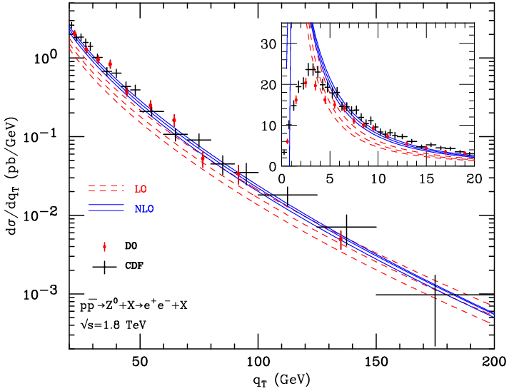
In Fig. 1 we plot the $q_{T}$ spectrum of Drell–Yan $e^{+}e^{-}$ pairs at the Tevatron Run I ($\sqrt{s}=1.8$ GeV) at LO and NLO accuracy. The bands are obtained by varying independently the factorization ($\mu_{F}$) and renormalization ($\mu_{R}$) scales in the range $0.5m_{Z}\leq\mu_{F},\mu_{R}\leq 2m_{Z}$, with the constraint $0.5\leq\mu_{F}/\mu_{R}\leq 2$. At the LO level, the scale dependence is about $\pm$25% at large $q_{T}$, it decreases as $q_{T}$ decreases, and it becomes about $\pm$15% at $q_{T}\sim 20$ GeV. The scale dependence at NLO is about $\pm$8% at $q_{T}\sim 20$ GeV, with a slight reduction at large $q_{T}$. We note that the LO and NLO bands do not overlap in the region where $q_{T}\raisebox{-2.58334pt}{\hbox to0.0pt{$\,\sim\,$\hss}}\raisebox{1.72218pt}{$\,<\,$}70$ GeV. This proves that, in this region of transverse momenta, the size of the band obtained through scale variations at LO definitely underestimates the theoretical uncertainty due to the missing NLO corrections.

The inset plot of Fig. 1 shows the $K$-factor, obtained by normalizing the NLO band with the LO result at $\mu_{F}=\mu_{R}=m_{Z}$. The impact of the NLO corrections, at central values of the scales, ranges from about +10% at $q_{T}\sim 200$ GeV to about +50% at $q_{T}\sim 20$ GeV.

In Fig. 2 we compare the results of the fixed-order calculations with CDF and D0 data. The experimental error bars reported in Fig. 2 include statistical and systematic contributions, but they do not include the overall normalization uncertainty due to the luminosity measurement. The CDF and D0 luminosity uncertainties are $\pm$3.9% and $\pm$4.4%, respectively. The corresponding cross sections are $\sigma_{\rm CDF}=248\pm 11$ pb [49] and $\sigma_{\rm D0}=221\pm 11$ pb [55], where the errors are dominated by the luminosity uncertainties. We note that, using the MRST2004 parton distribution functions [53] and including the effect of scale variations, the values of the QCD cross section at NLO and NNLO are $\sigma_{NLO}=226\pm 5$ pb and $\sigma_{NNLO}=236\pm 2$ pb, respectively.

From Fig. 2 we see that the NLO result is in agreement with the experimental data over a wide region of transverse momenta, from large to relatively-small values of $q_{T}$. In particular, in the region 20 GeV$\raisebox{-2.58334pt}{\hbox to0.0pt{$\,\sim\,$\hss}}\raisebox{1.72218pt}{$\,<\,$}q_{T}\raisebox{-2.58334pt}{\hbox to0.0pt{$\,\sim\,$\hss}}\raisebox{1.72218pt}{$\,<\,$}70$ GeV, the sizeable increase of the LO result produced by the NLO corrections is important to achieve the agreement between the data and the NLO calculation. In the small $q_{T}$ region, which is shown in the inset plot, the LO and NLO calculations do not describe the data. This is not unexpected since, when $q_{T}\rightarrow 0$, the LO and NLO cross section eventually diverges to $+\infty$ and $-\infty$, respectively. This is the region where the effects of soft-gluon resummation are essential and have to be taken into account.

A more effective comparison between the fixed-order calculations and the data can be performed by considering the fractional difference $(X-{\rm theory})/{\rm theory}$. We choose the NLO result at central value of the scales as ‘reference theory’ and we define the following fractional difference (see Fig. 3):

where the label $X$ refers to either the LO and NLO results, including scale variations (dashed and solid curves in Fig. 3), or the experimental data.

The perturbative QCD predictions at NLO have an associated theoretical uncertainty due to missing higher-order terms. By comparing the numerical results at LO and NLO, we can try to consistently estimate this uncertainty. At large values of $q_{T}$, the LO and NLO bands overlap. In this region of transverse momenta, we can thus use the scale variation band as uncertainty estimate: we obtain that the NLO predictions have a perturbative uncertainty of about $\pm$8%. As $q_{T}$ decreases below the value $q_{T}\sim 70$ GeV, the LO and NLO bands do not overlap (see Fig. 3), and this signals that scale variations (up to NLO) tend to underestimate the effect of higher-order contributions. To obtain a more reliable estimate of the uncertainty of the NLO central value, we assign it a theoretical error as given by its difference with respect to its closest value in the LO band (i.e., the value on the upper curve of the LO band in Fig. 3). Using this procedure, we obtain a NLO uncertainty that increases as $q_{T}$ decreases, and that reaches the value of about $\pm$20% at $q_{T}\sim 20$ GeV. In the region of smaller values of $q_{T}$, the LO and NLO results show a pathological behaviour. This behaviour, which is discussed below, prevents us from making a sensible quantitative estimate of the theoretical uncertainty of the NLO predictions. We can only draw a qualitative conclusions: the uncertainty of the NLO predictions systematically increases as $q_{T}$ decreases.

We know that, in the small-$q_{T}$ region, the convergence of the fixed-order perturbative expansion is spoiled by the presence of large logarithmic corrections. This behaviour is clearly seen in Fig. 3 by comparing the LO and NLO results at $q_{T}\sim 1$ GeV. We also recall that, as $q_{T}\rightarrow 0$, the LO cross section diverges to $+\infty$ whereas the NLO cross section diverges to $-\infty$. Since the NLO corrections increase the LO results at large $q_{T}$, the LO and NLO cross sections have to coincide at some intermediate value of $q_{T}$, before reaching the small-$q_{T}$ region where their different divergent behaviour sets in. The numerical agreement of the LO and NLO results occurs in the region where $q_{T}\sim$ 2–3 GeV (Fig. 3). Since this region is so close to that where the convergence of the fixed-order is definitely spoiled, it cannot be regarded as a region where the order-by-order expansion is well-behaved. Therefore, the systematic decrease of the difference between the LO and NLO cross sections when $q_{T}$ varies from about 20 GeV to 2–3 GeV is simply driven by the sickness of the LO and NLO results at smaller $q_{T}$. This decrease cannot be interpreted as an increase of the theoretical accuracy of the NLO predictions. The behaviour of the LO and NLO results below $q_{T}\sim 20$ GeV signals the necessity to include the effect of higher-order contributions and, eventually, of resummed calculations.

Having estimated the perturbative uncertainty of the NLO predictions, we can add some comments on the comparison with the experimental data (see Fig. 3). We consider the region where $q_{T}\raisebox{-2.58334pt}{\hbox to0.0pt{$\,\sim\,$\hss}}\raisebox{1.72218pt}{$\,>\,$}20$ GeV, since at smaller values of $q_{T}$ the NLO calculation looses predictivity. Throughout this region, the data agree with the NLO predictions. The experimental errors are typically larger (smaller) than the NLO uncertainty when $q_{T}\raisebox{-2.58334pt}{\hbox to0.0pt{$\,\sim\,$\hss}}\raisebox{1.72218pt}{$\,>\,$}70$ GeV ($20~{\rm GeV}\raisebox{-2.58334pt}{\hbox to0.0pt{$\,\sim\,$\hss}}\raisebox{1.72218pt}{$\,<\,$}q_{T}\raisebox{-2.58334pt}{\hbox to0.0pt{$\,\sim\,$\hss}}\raisebox{1.72218pt}{$\,<\,$}30$ GeV). The experimental errors and the corresponding NLO errors overlap, with the sole exception of a couple of D0 data points. We note that part of the differences between data and theory have a systematic component due to the luminosity uncertainties ($\pm$3.9% at CDF, and $\pm$4.4% at D0) and to the values of the total cross sections. The NLO predictions for $d\sigma/dq_{T}$ correspond to the value^∥∥ ∥ This value is obtained by convoluting the NNLO partonic cross sections with NLO parton distributions (see the comment above Eq. (13)). $\sigma=233$ pb of the total cross section; this value is about 6% smaller than the CDF value, and it is about 5% larger than the D0 value. Therefore, by inspection of Fig. 3, we see that considering the normalized distribution $\frac{1}{\sigma}\frac{d\sigma}{dq_{T}}$ (i.e. the shape of the $q_{T}$ spectrum) would lead to an overall improvement of the agreement between the CDF data, the D0 data and the NLO predictions.

The D0 collaboration has performed a measurement [51] of the normalized $q_{T}$ distribution, $\frac{1}{\sigma}\frac{d\sigma}{dq_{T}}$, from data at the Tevatron Run II (${\sqrt{s}}=1.96$ GeV). To obtain fixed-order QCD predictions for the normalized distribution, we have to consistently compute $d\sigma/dq_{T}$ and ${\sigma}$. The cross section $d\sigma/dq_{T}$ at NLO (LO) is computed by convoluting the corresponding NLO (LO) partonic cross sections with NLO (LO) parton distributions. These differential partonic cross sections at NLO (LO) contribute to the total partonic cross sections at NNLO (NLO). Therefore, to normalize $d\sigma/dq_{T}$ at NLO (LO), the total cross section $\sigma$ is computed by convoluting the total partonic cross sections at NNLO (NLO) with NLO (LO) parton distributions. In conclusion, our fixed-order calculations of the normalized $q_{T}$ distribution are obtained by using the following relation:

where the two factors, $1/\sigma$ and $d\sigma/dq_{T}$, on the right-hand side are evaluated with the same parton distributions and at the same values of the renormalization and factorization scales.

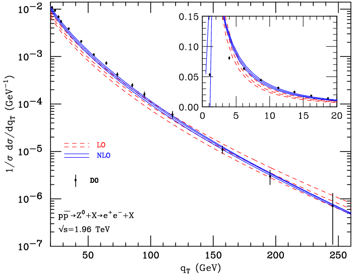
The D0 data and the LO and NLO results for the normalized distribution $\frac{1}{\sigma}\frac{d\sigma}{dq_{T}}$ at the Tevatron Run II are presented in Fig. 4. The LO and NLO bands are obtained by varying $\mu_{F}$ and $\mu_{R}$ in the same range as in the fixed-order calculations at Run I. The fractional difference $(X-{\rm theory})/{\rm theory}$ at Run II is shown in Fig. 5; this fractional difference differs from that in Eq. (12) by the sole replacement of $\frac{d\sigma}{dq_{T}}$ with $\frac{1}{\sigma}\frac{d\sigma}{dq_{T}}$.

Comparing Figs. 2 and 3 with Figs. 4 and 5, we can see that the overall features of the fixed-order results are unchanged in going from Run I to Run II. The main quantitative differences are due to the fact that, at Run II, we are considering the normalized $q_{T}$ distribution. The NLO corrections to $\frac{1}{\sigma}\frac{d\sigma}{dq_{T}}$ are smaller than the NLO corrections to $\frac{d\sigma}{dq_{T}}$. The scale dependence of the fixed-order results is only marginally reduced by considering $\frac{1}{\sigma}\frac{d\sigma}{dq_{T}}$ rather than $\frac{d\sigma}{dq_{T}}$.

The perturbative uncertainty of the NLO predictions at Run II can be estimated in the same way as at Run I. We conclude that the NLO error increases from about $\pm 6$–8% in the region where $q_{T}\raisebox{-2.58334pt}{\hbox to0.0pt{$\,\sim\,$\hss}}\raisebox{1.72218pt}{$\,>\,$}50$ GeV (see the size of the NLO band in Fig. 5) to about $\pm 15$% at $q_{T}\sim 20$ GeV (see the upper value of the LO band in Fig. 5). At smaller values of $q_{T}$ the NLO calculation looses predictivity. In the region where $q_{T}\raisebox{-2.58334pt}{\hbox to0.0pt{$\,\sim\,$\hss}}\raisebox{1.72218pt}{$\,>\,$}90$ GeV, the D0 data agree with the NLO predictions. In the region where $20~{\rm GeV}\raisebox{-2.58334pt}{\hbox to0.0pt{$\,\sim\,$\hss}}\raisebox{1.72218pt}{$\,<\,$}q_{T}\raisebox{-2.58334pt}{\hbox to0.0pt{$\,\sim\,$\hss}}\raisebox{1.72218pt}{$\,<\,$}90$ GeV, the experimental errors are typically smaller than the NLO uncertainty; in this region, three data points overshoot the NLO predictions (they differ by about two standard deviations from the upper value of the NLO uncertainty band).

We add a comment on the fixed-order calculations presented in the papers of the D0 collaboration. The labels “Fixed-order $({\cal O}(\alpha_{\mathrm{S}}^{2}))$” in Ref. [50] and “NNLO” in Ref. [51] refer to perturbative calculations that use the same NLO partonic cross sections of our NLO calculations. The differences between these calculations can be due to the use of different parton distributions and of different renormalization and factorization scales. In the region where $q_{T}\raisebox{-2.58334pt}{\hbox to0.0pt{$\,\sim\,$\hss}}\raisebox{1.72218pt}{$\,>\,$}20$ GeV, the fixed-order results of Refs. [50, 51] are systematically smaller than our NLO central values: the differences can reach the level of about 12% in the case of the “Fixed-order $({\cal O}(\alpha_{\mathrm{S}}^{2}))$” result (compare Fig. 26 of the second paper in Ref. [50] with our Fig. 3) and of about 7% in the case of the “NNLO” result (compare Fig. 2b in Ref. [51] with our Fig. 5). We note that the differences tend to reduce the agreement with the D0 data; we also note that these differences are consistent with our estimate of the perturbative uncertainty of the NLO predictions. This observation underlines the relevance of quantifying the uncertainty of the perturbative QCD predictions.

In the following we present our resummed results at NLL+LO accuracy and we compare them with the Tevatron data. To compute the hadronic cross sections, we use the MRST2004 NLO parton distributions [53], with $\alpha_{\mathrm{S}}$ evaluated at 2-loop order.

In the small-$q_{T}$ region, the use of NLO parton distributions is fully consistent with the NLL+LO accuracy of the partonic cross section. Indeed, at small values of $q_{T}$, the NLL+LO partonic cross section includes the complete perturbative expansion up to NLO (i.e., ${\cal O}(\alpha_{\mathrm{S}})$) and the resummation of the LL and NLL terms. The use of NLO parton distributions is justified also at intermediate values of $q_{T}$, where the calculation of the partonic cross section is driven by the small-$q_{T}$ resummation and constrained by the value of the total cross section at NLO.

The resummed calculation depends on the factorization and renormalization scales and on the resummation scale $Q$. As in fixed-order calculations, we choose $\mu_{F}=\mu_{R}=m_{Z}$ as central value. Factorization and renormalization scale uncertainties are computed as described in Sect. 3.1, by considering variations of $\mu_{F}$ and $\mu_{R}$ by a factor of two around (above and below) the central value. A similar procedure is applied to the resummation scale: we choose $Q=m_{Z}/2$ as central value and consider scale variations in the range $m_{Z}/4<Q<m_{Z}$. As discussed below, we regard this central value of the resummation scale and the corresponding range $m_{Z}/4<Q<m_{Z}$ as sufficiently conservative (e.g., more conservative than the range $m_{Z}/2<Q<2m_{Z}$) from a theoretical viewpoint^†† † Also in the case of Higgs boson production, we used [29] the range $m_{H}/4<Q<m_{H}$ ($m_{H}$ being the mass of the Higgs boson) to estimate the resummation scale uncertainty..

The resummed logarithmic terms depend on $Q$ through the variable ${\tilde{L}}$ in Eq. (7). This implies that the logarithmic contributions are mostly effective in the $b$-space region where $bQ\raisebox{-2.58334pt}{\hbox to0.0pt{$\,\sim\,$\hss}}\raisebox{1.72218pt}{$\,>\,$}1$, which corresponds to the transverse-momentum region where $q_{T}\raisebox{-2.58334pt}{\hbox to0.0pt{$\,\sim\,$\hss}}\raisebox{1.72218pt}{$\,<\,$}Q$. By decreasing $Q$, the resummation effects are depleted in the region where $q_{T}\raisebox{-2.58334pt}{\hbox to0.0pt{$\,\sim\,$\hss}}\raisebox{1.72218pt}{$\,>\,$}Q$ and enhanced in the region where $q_{T}\raisebox{-2.58334pt}{\hbox to0.0pt{$\,\sim\,$\hss}}\raisebox{1.72218pt}{$\,<\,$}Q$. The bulk of the $Z$ production cross section and, thus, the main effect of the logarithmic terms are located at values of $q_{T}$ that are certainly smaller than $m_{Z}$: indeed, we observe that the average transverse momentum of the $Z$ boson is of the order of $\alpha_{\mathrm{S}}(m_{Z})\,m_{Z}$. Therefore, it is physically sensible to use a central value of $Q$ that is smaller than $m_{Z}$. Nonetheless, too small values of $Q$ have to be avoided. As we have pointed out in Sect. 3.1, the fixed-order perturbative expansion shows instabilities (due to higher-order logarithmic corrections) in the region where $q_{T}\raisebox{-2.58334pt}{\hbox to0.0pt{$\,\sim\,$\hss}}\raisebox{1.72218pt}{$\,<\,$}20$ GeV. Therefore, in our NLL+LO calculation we should exclude values of $Q$ that are smaller than about 20 GeV. In this respect, a value of $Q$ as low as $Q\sim m_{Z}/4$ can be regarded as a conservative value from a perturbative viewpoint. The NLL+LO calculation with such a value of $Q$ will be closer to the corresponding fixed-order calculation throughout region of intermediate values of $q_{T}$ where the fixed-order expansion is relatively well behaved.

The NLL+LO $q_{T}$ spectrum at the Tevatron ($\sqrt{s}=1.8$ TeV) is presented in Fig. 6. In the left panel, the NLL+LO result (solid line) at the default scales ($\mu_{F}=\mu_{R}=m_{Z}$, $Q=m_{Z}/2$) is compared with the corresponding ^‡‡ ‡ Here and in the inset plot of Figs. 8, the LO result refers to the convolution of the partonic cross section at LO with the parton distributions at NLO. This LO result thus differs from the customary LO calculation, which uses parton distributions at LO and is presented in Sect. 3.1. Incidentally, we note that the difference produced by using NLO vs. LO parton distributions is much smaller than the scale uncertainty of the corresponding results. We find that the difference is below the level of about $\pm 2$% ($-6$%) if $20~\rm{GeV}\raisebox{-2.58334pt}{\hbox to0.0pt{$\,\sim\,$\hss}}\raisebox{1.72218pt}{$\,<\,$}q_{T}\raisebox{-2.58334pt}{\hbox to0.0pt{$\,\sim\,$\hss}}\raisebox{1.72218pt}{$\,<\,$}140~\rm{GeV}$ ($140~\rm{GeV}\raisebox{-2.58334pt}{\hbox to0.0pt{$\,\sim\,$\hss}}\raisebox{1.72218pt}{$\,<\,$}q_{T}\raisebox{-2.58334pt}{\hbox to0.0pt{$\,\sim\,$\hss}}\raisebox{1.72218pt}{$\,<\,$}200~\rm{GeV}$). LO result (dashed line). We observe that soft-gluon resummation leads to a well-behaved distribution: it vanishes as $q_{T}\rightarrow 0$, has a kinematical peak at $q_{T}\sim 2$ GeV, and tends to the corresponding LO result at larger values of $q_{T}$. The LO finite component of the spectrum (see Eq. (2)), rescaled by a factor of 10 to make it more visible, is also shown for comparison (dotted line). This component smoothly vanishes as $q_{T}\rightarrow 0$ and gives a small contribution to the NLL+LO result in the low-$q_{T}$ region. The contribution is smaller than 1% at the peak and becomes more important as $q_{T}$ increases: it is about 8% at $q_{T}\sim 20$ GeV, about 20% at $q_{T}\sim 30$ GeV and about 60% at $q_{T}\sim 50$ GeV. A similar quantitative behaviour is observed by considering the contribution of the LO finite component to the LO result; the contribution is about 13% at $q_{T}\sim 20$ GeV, about 30% at $q_{T}\sim 30$ GeV and about 75% at $q_{T}\sim 50$ GeV. In the region of intermediate values of $q_{T}$ (say, around 20 GeV), the difference between the NLL+LO and LO results is much larger than the size of the LO finite component. This difference is produced by the logarithmic terms (at NLO and beyond NLO) that are included in the resummed calculation at NLL accuracy. At large values of $q_{T}$ the contribution of the LO finite component sizeably increases. This behaviour indicates that the logarithmic terms are no longer dominant and that the resummed calculation cannot improve upon the predictivity of the fixed-order expansion.

In the right panel of Fig. 6 we show the scale dependence of the NLL+LO result. The band (dashed lines) is obtained by varying the renormalization and factorization scales as described in Sect. 3.1. Although $\mu_{R}$ and $\mu_{F}$ are varied independently, we find that the dependence on $\mu_{R}$ dominates at any values of $q_{T}$. In the region of small and intermediate values of $q_{T}$, the scale dependence of the NLL+LO result is definitely much smaller than the difference between the NLL+LO and LO results. The scale dependence of the resummed result is about $\pm 5$% at the peak, and it increases to $\pm 9$% at $q_{T}\sim 50$ GeV.

The renormalization/factorization scale dependence of the NLL+LO spectrum (the band enclosed by the solid lines) is more clearly visible in Fig. 7. Here the CDF and D0 data at Tevatron Run I are also superimposed on the NLL+LO result. There is an overall agreement between the data and the resummed calculation in the region from small to intermediate values of $q_{T}$. In particular, the agreement tends to improve by decreasing the value of $\mu_{R}$ from $\mu_{R}=m_{Z}$ to $\mu_{R}=m_{Z}/2$. The inset plot shows the region of intermediate and large values of $q_{T}$. At large $q_{T}$, the NLL+LO result deviates from the data, and the deviation increases as $q_{T}$ increases. As previously observed on purely theoretical grounds, the NLL+LO calculation looses predictivity in the large-$q_{T}$ region. The lost of predictivity is also signalled by the systematic increase of the scale dependence, whose size is about $\pm 9$% at $q_{T}\sim 50$ GeV and becomes about $\pm 22$% at $q_{T}\sim 90$ GeV. As we shall see in the next figure, at large values of $q_{T}$, the dependence on the resummation scale $Q$ is even stronger than the dependence on $\mu_{R}$ and $\mu_{F}$.

In Fig. 8 we show how the NLL+LO result depends on the resummation scale $Q$. We fix $\mu_{R}=\mu_{F}=m_{Z}$, and we present the result of the NLL+LO calculation at three different values of the resummation scale: $Q=m_{Z}$ (dashed line), $Q=m_{Z}/2$ (solid line) and $Q=m_{Z}/4$ (dot-dashed line). In the region of small and intermediate values of $q_{T}$, large values of $Q$ ($Q\sim m_{Z},m_{Z}/2$) lead to a better agreement with the experimental data. In this region, the $q_{T}$ spectrum at NLL+LO becomes softer by decreasing the value of $Q$. This behaviour is not unexpected. The resummed calculation cures the instabilities of the fixed-order calculations by implementing the physical transverse-momentum smearing produced by soft multiparton radiation. The size of the $q_{T}$ region where the smearing takes place is controlled by the value of $Q$. By increasing $Q$, the resummation smearing is extended to larger values of $q_{T}$, and the $q_{T}$ spectrum becomes harder.

The inset plot of Fig. 8 refers to the region of intermediate and large values of $q_{T}$. We present the NLL+LO results and the corresponding LO result (dotted line), which does not depend on $Q$. Considering large values of $Q$ ($Q\sim m_{Z},m_{Z}/2$), the NLL+LO results follow the data up to $q_{T}\sim 50$ GeV and deviates from the data at larger values of $q_{T}$. At large $q_{T}$, the deviation decreases if we consider the NLL+LO calculation with smaller values of $Q$. We also notice that the LO result is approximated better by the NLL+LO calculation if $Q$ is smaller. This fact is not surprising. Varying $Q$, we smoothly set the transverse-momentum scale below which the resummed logarithmic terms are mostly effective; if $Q$ is smaller, the resummation effects are confined to a range of smaller values of $q_{T}$. Independently of these observations, the sizeable $Q$ dependence of the resummed calculation at large $q_{T}$ confirms the lost of predictivity of the NLL+LO result in this transverse-momentum region.

The variations of the NLL+LO cross section produced by varying the resummation scale give further insight on the size of yet uncalculated higher-order logarithmic contributions at small and intermediate values of $q_{T}$. To quantify the resummation scale uncertainty on the cross section, we choose $Q=m_{Z}/2$ as central value and vary $Q$ between $m_{Z}$ and $m_{Z}/4$. We find that the uncertainty is about $\pm 12$% in the region of the peak, it decreases in the region around $q_{T}\sim 5$ GeV, and then it increases to about $\pm 15$% in the region where $q_{T}\sim 20$ GeV.

The integral over $q_{T}$ of the NLL+LO spectrum is in agreement (for any values of $\mu_{R},\mu_{F}$ and $Q$) with the value of the NLO total cross section to better than 1%, thus checking the numerical accuracy of our code. We also note that the large-$q_{T}$ region gives a little contribution to the total cross section; therefore, the total cross section constraint mainly acts as a perturbative constraint on the NLL+LO spectrum in the region from intermediate to small values of $q_{T}$. To confirm this statement at the quantitative level, we consider the cross section ratio $\sigma(q_{T{\rm max}})/\sigma$, where $\sigma(q_{T{\rm max}})$ is the contribution to the total cross section $\sigma$ from the transverse-momentum region where $q_{T}\leq q_{T{\rm max}}$. The cross section $\sigma(q_{T{\rm max}})$ can be computed either at the NLO or at NLL+LO accuracy (i.e. by integration of the NLL+LO spectrum over $q_{T}$). Provided $q_{T{\rm max}}$ is not small, we find that the NLO and NLL+LO values of $\sigma(q_{T{\rm max}})$ are very close and that $\sigma(q_{T{\rm max}})$ constitutes a large fraction of $\sigma$. For example, the NLO (NLL+LO) value of the cross section ratio is $\sigma(q_{T{\rm max}})/\sigma=0.86\,(0.87)$ at $q_{T{\rm max}}=20$ GeV and $\sigma(q_{T{\rm max}})/\sigma=0.93\,(0.94)$ at $q_{T{\rm max}}=30$ GeV. The resummation scale uncertainty of $\sigma(q_{T{\rm max}})$ at NLL+LO accuracy is about $\pm 2$% at $q_{T{\rm max}}=20$ GeV, and it is below the 1% level in the region where $q_{T{\rm max}}\raisebox{-2.58334pt}{\hbox to0.0pt{$\,\sim\,$\hss}}\raisebox{1.72218pt}{$\,>\,$}30$ GeV.

In analogy with our presentation of the fixed-order results in Sect. 3.1, we consider the resummed results and introduce a corresponding fractional difference $(X-{\rm theory})/{\rm theory}$. Now, at variance with Eq. (12), we choose the NLL+LO result at central value of the scales as ‘reference theory’ and we define the following fractional difference:

where the label $X$ refers to either the experimental data or the NLL+LO result at various values of the scales.

This fractional difference is shown in Fig. 9. The band enclosed by the solid lines corresponds to our computation of the scale uncertainty. It includes the combined effect from varying $\mu_{F},\mu_{R}$ and $Q$ as previously described. We find that the resummation scale uncertainty is larger than the factorization/renormalization scale uncertainty at (almost) all values of $q_{T}$. We comment on the results in Fig. 9 by considering various regions of transverse momenta in turn.

We first consider the large-$q_{T}$ region. At $q_{T}\sim 40$ GeV, the scale uncertainty of the NLL+LO result is of about $\pm 20$%. At high $q_{T}$, the scale uncertainty is definitely larger and quickly increases as $q_{T}$ increases. The decrease of the scale uncertainty in the region around $q_{T}\sim 60$ GeV has no physical interpretation: it has to be regarded as an accidental fact rather than a reduction of the theoretical uncertainty. Comparing the uncertainty of the NLL+LO calculation with that of the fixed-order calculations (see Sect. 3.1), we thus conclude that, in the large-$q_{T}$ region, the NLL+LO predictions are less accurate than the NLO predictions.

In the region of intermediate values of $q_{T}$, the scale uncertainty of the NLL+LO result is moderate (see Fig. 9). In this region it is appropriate to perform a more detailed comparison between the NLL+LO calculation and the fixed-order calculations. We consider Eq. (12), which uses the NLO central value as ‘reference theory’, and we compute the fractional difference of the NLL+LO calculation. The results are presented in Fig. 10, which shows the NLL+LO calculation at central value of the scales (central dot-dashed line) and the corresponding scale uncertainty (upper and lower dot-dashed lines). The NLO (solid lines) and LO (dashed lines) bands in Fig. 10 are exactly the same bands as those in Fig. 3. In the region where $10~{\rm GeV}\raisebox{-2.58334pt}{\hbox to0.0pt{$\,\sim\,$\hss}}\raisebox{1.72218pt}{$\,<\,$}q_{T}\raisebox{-2.58334pt}{\hbox to0.0pt{$\,\sim\,$\hss}}\raisebox{1.72218pt}{$\,<\,$}40~{\rm GeV}$, the NLL+LO and NLO central values are quite close: their difference is, at most, of about 8%. Decreasing the value of $q_{T}$, the scale uncertainty at NLL+LO decreases from about $\pm 20$% ($q_{T}\sim 40$ GeV), to about $\pm 15$% ($q_{T}\sim 20$ GeV) and $\pm 10$% ($q_{T}\sim 10$ GeV). We also recall our conclusions (see Sect. 3.1) about the uncertainty of the fixed-order perturbative expansion: the perturbative uncertainty of the NLO predictions is at the level of about $\pm 20$% in the region where $20~{\rm GeV}\raisebox{-2.58334pt}{\hbox to0.0pt{$\,\sim\,$\hss}}\raisebox{1.72218pt}{$\,<\,$}q_{T}\raisebox{-2.58334pt}{\hbox to0.0pt{$\,\sim\,$\hss}}\raisebox{1.72218pt}{$\,<\,$}40~{\rm GeV}$ (see the upper line of the LO band), and it does not decrease at smaller values of $q_{T}$. We conclude that, at intermediate values of $q_{T}$, the NLL+LO and NLO results are fully consistent and have a comparable perturbative uncertainty. The NLL+LO calculation provides us with QCD predictions that can be extended to smaller values of $q_{T}$ ($q_{T}\raisebox{-2.58334pt}{\hbox to0.0pt{$\,\sim\,$\hss}}\raisebox{1.72218pt}{$\,<\,$}20~{\rm GeV}$) with a controllable and relatively-small perturbative uncertainty.

The bulk of the production cross section is contained in the small-$q_{T}$ region. Considering the region above the peak of the $q_{T}$ distribution ($2~{\rm GeV}\raisebox{-2.58334pt}{\hbox to0.0pt{$\,\sim\,$\hss}}\raisebox{1.72218pt}{$\,<\,$}q_{T}\raisebox{-2.58334pt}{\hbox to0.0pt{$\,\sim\,$\hss}}\raisebox{1.72218pt}{$\,<\,$}20~{\rm GeV}$), the scale uncertainty of the NLL+LO calculation is below the level of about $\pm 15$% (Fig. 9). The size of the scale uncertainty increases in the region below the peak. The effect of the scale variations is larger in the region below the peak since the shape of the $q_{T}$ distribution is much steeper in this region (see Figs. 7 and 8). Note also that this region is expected to be most sensitive to NP effects. The sizeable reduction of the scale uncertainty in the interval $q_{T}\sim 3$–7 GeV can be accidental and, thus, it can underestimate the perturbative uncertainty of the NLL+LO result.

The detailed comparison in Fig. 9 shows that the experimental data are consistent with the NLL+LO predictions in the small-$q_{T}$ region. As in the case of Fig. 3, we also recall that part of the differences between data and theory have a systematic component due to the luminosity uncertainties and to the values of the total cross sections. In particular, the central value of $d\sigma/dq_{T}$ at NLL+LO accuracy corresponds to the NLO values, $\sigma=226$ pb, of the total cross section; this value is about 9% smaller than the CDF value, and it is about 2% larger than the D0 value. These differences between the total cross sections are consistent with the fact that the NLL+LO result tends to agree better with the D0 data than with the CDF data.

The quantitative predictions presented up to now are obtained in a purely perturbative framework. It is known (see e.g. Ref. [13] and references therein) that the transverse-momentum distribution is affected by NP effects, which become important as $q_{T}$ becomes small. A customary way of modelling these effects is to introduce an NP transverse-momentum smearing of the distribution. In the case of resummed calculations in impact parameter space, the NP smearing is implemented by multiplying the $b$-space perturbative form factor by an NP form factor. Different procedures to relate the two form factors and several different parametrizations of the NP form factor are available in the literature [39, 56, 23]; the corresponding NP parameters are obtained by global fits to DY data [23, 27, 57].

A detailed study of the NP effects is beyond the aim of this work. We limit ourselves to illustrate the possible impact of NP effects on our resummed calculation. To this purpose, we simply multiply the $b$-space resummation factor ${\cal W}_{N}^{V}(b,M)$ (see Eqs. (3) and (4)) by a NP factor, $S_{NP}$, which includes a gaussian smearing of the form

In Fig. 11 we show the NLL+LO distribution at central values of the scales with (solid) and without (dashed) the inclusion of the NP factor. The numerical value of the NP coefficient $g_{NP}$ is taken to be $g_{NP}=0.8~{\rm GeV}^{2}$ [25]. Using this values of $g_{NP}$, the NP effects reduce (increase) the perturbative distribution where $q_{T}\raisebox{-2.58334pt}{\hbox to0.0pt{$\,\sim\,$\hss}}\raisebox{1.72218pt}{$\,<\,$}3$ GeV ($q_{T}\raisebox{-2.58334pt}{\hbox to0.0pt{$\,\sim\,$\hss}}\raisebox{1.72218pt}{$\,>\,$}3$ GeV). For instance, the NP correction is about $-10$% at $q_{T}\sim 2$ GeV, about $+8$% at $q_{T}\sim 5$ GeV, and it is smaller than $+4$% where $q_{T}\raisebox{-2.58334pt}{\hbox to0.0pt{$\,\sim\,$\hss}}\raisebox{1.72218pt}{$\,>\,$}10$ GeV. As expected, the effect of the NP form factor is to make the distribution harder, thus improving the agreement with the experimental data at very small values of $q_{T}$. On the basis of the results in Ref. [29], we also expect that such NP effect is qualitatively similar to that produced by the inclusion of higher-order logarithmic contributions. This expectation is consistent with the fact that the quantitative impact of the NP form factor is within the perturbative uncertainty of the NLL+LO result (see Figs. 8 and 9). A detailed comparison of Tevatron data with a full NNLL+NLO calculation, including non-perturbative effects, is left to future work.

We have repeated our NLL+LO study by considering the normalized $q_{T}$ distribution, $\frac{1}{\sigma}\frac{d\sigma}{dq_{T}}$, at the Tevatron Run II. The main features of the results are definitely very similar to those at Run I. The NLL+LO results at small and intermediate values of $q_{T}$ are briefly summarized in Fig. 12. We show the NLL+LO distribution at central values of the scales with (solid) and without (dashed) the inclusion of the NP form factor (we use the same values of $g_{NP}$ as in Fig. 11). Since the perturbative uncertainty is dominated by the effect of varying the resummation scale $Q$, we fix $\mu_{R}=\mu_{F}=m_{Z}$ and we also show the NLL+LO results with $Q=m_{Z}$ (dotdashed) and $Q=m_{Z}/4$ (dotted). We observe that the D0 data are consistent with the NLL+LO predictions. We also observe that the experimental errors are smaller than the uncertainty of the NLL+LO results, thus demanding more accurate perturbative predictions.

References

- [1] R. Hamberg, W. L. van Neerven and T. Matsuura, Nucl. Phys. B 359 (1991) 343 [Erratum-ibid. B 644 (2002) 403]; R. V. Harlander and W. B. Kilgore, Phys. Rev. Lett. 88 (2002) 201801.
- [2] C. Anastasiou, L. J. Dixon, K. Melnikov and F. Petriello, Phys. Rev. D 69 (2004) 094008.
- [3] K. Melnikov and F. Petriello, Phys. Rev. Lett. 96 (2006) 231803, Phys. Rev. D 74 (2006) 114017.
- [4] S. Dittmaier and M. Kramer, Phys. Rev. D 65 (2002) 073007; U. Baur and D. Wackeroth, Phys. Rev. D 70 (2004) 073015; V. A. Zykunov, Phys. Atom. Nucl. 69 (2006) 1522 [Yad. Fiz. 69 (2006) 1557]; A. Arbuzov et al., Eur. Phys. J. C 46 (2006) 407 [Erratum-ibid. C 50 (2007) 505]; C. M. Carloni Calame, G. Montagna, O. Nicrosini and A. Vicini, JHEP 0612 (2006) 016.
- [5] U. Baur, O. Brein, W. Hollik, C. Schappacher and D. Wackeroth, Phys. Rev. D 65 (2002) 033007; V. A. Zykunov, Phys. Rev. D 75 (2007) 073019; C. M. Carloni Calame, G. Montagna, O. Nicrosini and A. Vicini, JHEP 0710 (2007) 109; A. Arbuzov et al., Eur. Phys. J. C 54 (2008) 451.
- [6] R. K. Ellis, G. Martinelli and R. Petronzio, Nucl. Phys. B 211 (1983) 106.
- [7] P. B. Arnold and M. H. Reno, Nucl. Phys. B 319 (1989) 37 [Erratum-ibid. B 330 (1990) 284].
- [8] R. J. Gonsalves, J. Pawlowski and C. F. Wai, Phys. Rev. D 40 (1989) 2245.
- [9] Y. L. Dokshitzer, D. Diakonov and S. I. Troian, Phys. Lett. B 79 (1978) 269, Phys. Rep. 58 (1980) 269.
- [10] G. Parisi and R. Petronzio, Nucl. Phys. B 154 (1979) 427.
- [11] G. Curci, M. Greco and Y. Srivastava, Nucl. Phys. B 159 (1979) 451.
- [12] J. C. Collins and D. E. Soper, Nucl. Phys. B 193 (1981) 381 [Erratum-ibid. B 213 (1983) 545].
- [13] J. C. Collins and D. E. Soper, Nucl. Phys. B 197 (1982) 446.
- [14] J. Kodaira and L. Trentadue, Phys. Lett. B 112 (1982) 66, report SLAC-PUB-2934 (1982), Phys. Lett. B 123 (1983) 335.
- [15] G. Altarelli, R. K. Ellis, M. Greco and G. Martinelli, Nucl. Phys. B 246 (1984) 12.
- [16] J. C. Collins, D. E. Soper and G. Sterman, Nucl. Phys. B 250 (1985) 199.
- [17] S. Catani, D. de Florian and M. Grazzini, Nucl. Phys. B 596 (2001) 299.
- [18] P. B. Arnold and R. P. Kauffman, Nucl. Phys. B 349 (1991) 381.
- [19] C. Balazs, J. w. Qiu and C. P. Yuan, Phys. Lett. B 355 (1995) 548.
- [20] C. Balazs and C. P. Yuan, Phys. Rev. D 56 (1997) 5558.
- [21] R. K. Ellis, D. A. Ross and S. Veseli, Nucl. Phys. B 503 (1997) 309.
- [22] R. K. Ellis and S. Veseli, Nucl. Phys. B 511 (1998) 649.
- [23] J. w. Qiu and X. f. Zhang, Phys. Rev. Lett. 86 (2001) 2724, Phys. Rev. D 63 (2001) 114011.
- [24] A. Kulesza and W. J. Stirling, Eur. Phys. J. C 20 (2001) 349.
- [25] A. Kulesza, G. Sterman and W. Vogelsang, Phys. Rev. D 66 (2002) 014011.
- [26] E. L. Berger and J. w. Qiu, Phys. Rev. D 67 (2003) 034026, Phys. Rev. Lett. 91 (2003) 222003.
- [27] F. Landry, R. Brock, P. M. Nadolsky and C. P. Yuan, Phys. Rev. D 67 (2003) 073016.
- [28] S. Berge, P. M. Nadolsky and F. I. Olness, Phys. Rev. D 73 (2006) 013002.
- [29] G. Bozzi, S. Catani, D. de Florian and M. Grazzini, Nucl. Phys. B 737 (2006) 73.
- [30] G. Bozzi, S. Catani, D. de Florian and M. Grazzini, Phys. Lett. B 564 (2003) 65.
- [31] G. Bozzi, S. Catani, D. de Florian and M. Grazzini, Nucl. Phys. B 791 (2008) 1.
- [32] M. Grazzini, JHEP 0601 (2006) 095.
- [33] R. Frederix and M. Grazzini, Phys. Lett. B 662 (2008) 353.
- [34] G. Bozzi, B. Fuks and M. Klasen, Phys. Rev. D 74 (2006) 015001.
- [35] H. Kawamura, J. Kodaira, H. Shimizu and K. Tanaka, Prog. Theor. Phys. 115 (2006) 667; H. Kawamura, J. Kodaira and K. Tanaka, Nucl. Phys. B 777 (2007) 203, Prog. Theor. Phys. 118 (2007) 581, Phys. Lett. B 662 (2008) 139.
- [36] Y. Koike, J. Nagashima and W. Vogelsang, Nucl. Phys. B 744 (2006) 59.
- [37] S. Catani, E. D’Emilio and L. Trentadue, Phys. Lett. B 211 (1988) 335.
- [38] C. T. H. Davies and W. J. Stirling, Nucl. Phys. B 244 (1984) 337.
- [39] C. T. H. Davies, B. R. Webber and W. J. Stirling, Nucl. Phys. B 256 (1985) 413.
- [40] D. de Florian and M. Grazzini, Phys. Rev. Lett. 85 (2000) 4678, Nucl. Phys. B 616 (2001) 247.
- [41] S. Catani and M. Grazzini, Phys. Rev. Lett. 98 (2007) 222002, and preprint in preparation.
- [42] A. Vogt, Phys. Lett. B 497 (2001) 228; C. F. Berger, Phys. Rev. D 66 (2002) 116002.
- [43] S. Moch, J. A. M. Vermaseren and A. Vogt, Nucl. Phys. B 688 (2004) 101.
- [44] S. Frixione and B. R. Webber, JHEP 0206 (2002) 029; S. Frixione, P. Nason and B. R. Webber, JHEP 0308 (2003) 007.
- [45] S. Alioli, P. Nason, C. Oleari and E. Re, JHEP 0807 (2008) 060.
- [46] K. Hamilton, P. Richardson and J. Tully, JHEP 0810 (2008) 015.
- [47] E. Laenen, G. Sterman and W. Vogelsang, Phys. Rev. Lett. 84 (2000) 4296.
- [48] S. Catani, M. L. Mangano, P. Nason and L. Trentadue, Nucl. Phys. B 478 (1996) 273.
- [49] A. A. Affolder et al. [CDF Collaboration], Phys. Rev. Lett. 84 (2000) 845.
- [50] B. Abbott et al. [D0 Collaboration], Phys. Rev. Lett. 84 (2000) 2792, Phys. Rev. D 61 (2000) 032004.
- [51] V. M. Abazov et al. [D0 Collaboration], Phys. Rev. Lett. 100 (2008) 102002.
- [52] A. D. Martin, R. G. Roberts, W. J. Stirling and R. S. Thorne, Eur. Phys. J. C 28 (2003) 455.
- [53] A. D. Martin, R. G. Roberts, W. J. Stirling and R. S. Thorne, Phys. Lett. B 604 (2004) 61.
- [54] J. Campbell, R.K. Ellis, MCFM - Monte Carlo for FeMtobarn processes, http://mcfm.fnal.gov.
- [55] B. Abbott et al. [D0 Collaboration], Phys. Rev. D 61 (2000) 072001.
- [56] G. A. Ladinsky and C. P. Yuan, Phys. Rev. D 50 (1994) 4239; F. Landry, R. Brock, G. Ladinsky and C. P. Yuan, Phys. Rev. D 63 (2001) 013004; S. Berge, P. M. Nadolsky, F. Olness and C. P. Yuan, Phys. Rev. D 72 (2005) 033015.
- [57] A. Kulesza and W. J. Stirling, JHEP 0312 (2003) 056; A. V. Konychev and P. M. Nadolsky, Phys. Lett. B 633 (2006) 710.