跳到论文正文
W Papers独立论文阅读器 arXiv:0812.2797 论文正文 计算阅读时间 · 0%
引用这篇论文根据当前论文元数据生成,正式投稿前建议核对。


License: arXiv.org perpetual non-exclusive license
arXiv:0812.2797v2 [hep-lat] 18 Sep 2009

The Chiral Condensate in a Finite Volume

Poul  H. Damgaard Affiliation:  The Niels Bohr International Academy, The Niels Bohr Institute, Blegdamsvej 17 DK-2100 Copenhagen Ø Denmark    Hidenori Fukaya Email: hfukaya@nbi.dk Affiliation:  The Niels Bohr International Academy, The Niels Bohr Institute, Blegdamsvej 17 DK-2100 Copenhagen Ø Denmark Affiliation:  High Energy Accelerator Research Organization (KEK), Tsukuba 305-0801, JapanEmail: , , Email: phdamg@nbi.dk
Abstract: 

Chiral perturbation theory at finite four-volume V(=L3​T)V(=L^{3}T) is reconsidered with a view towards finding a computational scheme that can deal with any value of Mπ​LM_{\pi}L, where MπM_{\pi} is a generic Nambu-Goldstone mass. The momentum zero modes that cause the usual pp-expansion to fail in the chiral limit are treated separately, and partly integrated out to all orders. In this way the theory remains infrared finite in the perturbative expansion, and the chiral limit can be considered at finite volume. We illustrate the technique by computing the quark condensate in a finite volume, smoothly connecting standard results in the pp-regime for larger masses with those of the ϵ\epsilon-regime for smaller masses. From the partially quenched theory we also obtain the spectral density of the Dirac operator, a smooth function from the microscopic region to the bulk region of the pp-regime.

1 Introduction

A number of studies have been devoted to the finite volume effects in low-energy QCD, or chiral perturbation theory (ChPT) [1]-[5]. The resulting finite-size scaling theory in ChPT has broad theoretical interest as it describes the critical behavior of dynamical symmetry breaking, and as such has corresponding applications in statistical physics as well. In lattice gauge theory it is certainly of great practical value to have analytical predictions for finite volumes available, as they can help in eliminating uncertainties due to the finite sizes used in numerical simulations [6].

To investigate the finite-size behavior of ChPT, essentially two perturbative approaches have been proposed so far [1]. One is the pp-expansion, which has just the same form as the perturbative series in an infinite volume, only replacing momentum integrals by the discrete sums over momentum due to the quantization in units of 1/L1/L (where LL is the linear extent). If we denote by MπM_{\pi} the mass of a generic (pseudo) Nambu-Goldstone boson, this pp-expansion is valid when Mπ​L≫1M_{\pi}L\gg 1. It is well known what happens when one takes the chiral limit in a volume such that Mπ​LM_{\pi}L crosses unity and gets even smaller [1, 2]: The propagators of the pseudo Nambu-Goldstone bosons blow up for one single momentum mode, the one of zero four-momentum. This invalidates the usual perturbative expansion, and a different technique is required. A solution to this problem was given in [1] in terms of a so-called ϵ\epsilon-expansion. In this scheme the zero-momentum mode is, in a sense that becomes more clear below, integrated out exactly, while all the remaining momentum modes are treated perturbatively. Since the chiral Lagrangian involves an infinite series of terms, and since it is only the perturbative expansion that is jeopardized, “exact” integration here refers to the term that is leading order in the quark masses mm.

The ϵ\epsilon-expansion is thus perfectly suited for studying the extreme case where the quark mass mm is so small that the pion Compton wave length overcomes the size of the volume, Mπ​L≪1M_{\pi}L\ll 1. Since the zero-mode becomes dominant in this ϵ\epsilon-regime, physical observables are mostly dependent on the leading low-energy constants: the infinite-volume chiral condensate Σ\Sigma and the pion decay constant FF, both in the chiral limit. The next-to-leading order terms (with coefficients LiL_{i}’s) at infinite volume are treated in perturbative fashion. This is similar to the pp-regime expansion, but the ordering of terms is different. Also in this respect, the ϵ\epsilon-regime provides an intriguing alternative to more conventional ChPT since different parts of the chiral theory are being probed to any given order. We note that the studies have now also been extended to Wilson ChPT where one has more terms which explicitly break the symmetry [7].

As the ϵ\epsilon-regime deals with the extremely chiral limit where non-trivial finite-size scaling starts to appear (but still far from the symmetric phase since one keeps L≫1/ΛQCDL\gg 1/\Lambda_{\rm QCD}), universality is at work. Perhaps the most important example of this is the equivalence of the zero-mode or vacuum part of the theory to chiral Random Matrix Theory (ChRMT) [8, 9]. Little is known in detail on how these universal phenomena cease and the ones depending on the dynamics specific to QCD appear when the quark mass increases and MπM_{\pi} becomes of order 1/L1/L [10]. In particular, it is not known precisely how the spectral density of the Dirac operator, described by ChRMT in the low end matches on to the spectrum at larger scales, in the pp-regime [11]-[13].

Recent developments in both computational facilities and algorithms have allowed simulations of full lattice QCD near the chiral limit, but no study has until now reached deep inside the ϵ\epsilon-regime except at rather strong coupling. Although results have often compared favorably to the ϵ\epsilon-expansion of ChPT, there may still be large systematic errors due to the condition Mπ​L≪1M_{\pi}L\ll 1 not being well fulfilled (see, e.g.e.g., ref. [14]). One might therefore ask whether it is possible to have a new approach which smoothly connects the pp-expansion and ϵ\epsilon-expansion and which remains valid even in the region Mπ​L∼1M_{\pi}L\sim 1. Recently, steps have been taken in that direction by means of a so-called mixed expansion [15, 16] (see also ref. [17]), where one treats the very light flavors with the counting rules of the ϵ\epsilon-expansion, while heavier flavors are counted according to the pp-expansion. The results turned out to be mixtures of the properties of the ϵ\epsilon and pp regimes: zero-mode fluctuations from the light sector in addition to 1-loop corrections from the heavier sector that include chiral logs and some of the LiL_{i}’s. But Refs. [15, 16] treated the light and heavy flavors separately and did not attack directly the regime where Mπ​L∼1M_{\pi}L\sim 1. Actually, two regimes at play here: one is the first obvious threshold when Mπ∼1/LM_{\pi}\sim 1/L, the other is when Mπ∼1/L2M_{\pi}\sim 1/L^{2}, the scale of the ϵ\epsilon-regime. The question is what happens in-between.

In this paper, we suggest a new perturbative approach where all the terms in the pp-expansion are kept but the zero mode is treated in exactly same way as in the ϵ\epsilon-expansion11 1 We understand that F. Niedermayer (unpublished) has considered an analogous scheme in the context of the O⁡(n)O(n) sigma model.. The expansion thus considers the zero momentum mode on a different footing from the rest, partially resumming terms to all orders. Before reaching the ϵ\epsilon-regime this means that an infinite series of terms that are normally considered in the perturbative expansion are included to all orders. The result is a slightly re-ordered perturbation theory expansion that is free from perturbative infrared singularities in the chiral limit. As an example, we compute here a formula for the chiral condensate which smoothly connects the results of the pp-regime [18] and the ϵ\epsilon-regime. We will argue that our formula is reliable even in the intermediate region where we go from Mπ∼1/LM_{\pi}\sim 1/L to Mπ∼1/L2M_{\pi}\sim 1/L^{2}.

Using the partial quenching technique based on replicas, we can treat a general theory with valence flavors and physical sea quark flavors of masses which are non-degenerate. This allows us to take the discontinuity on the imaginary axis of the valence quarks, and thus obtain the corresponding spectral density of the Dirac operator. It is also given by a smooth formula that connects known results in the ϵ\epsilon-regime [9] and pp-regime [11, 12].

The rest of our paper is organized as follows. In Section 2, we describe in detail our new perturbative method in ChPT. The chiral condensate to next-leading order is calculated in Section 3. Taking the discontinuity on the imaginary axis, we obtain the spectral density of the Dirac operator in Section 4. We show in Section 5 that our results provide a smooth connection between the ϵ\epsilon and pp regimes. In Section 6 we present some numerical examples which are useful when comparing with lattice QCD simulations. Conclusions and an outlook are given in Section 7.

2 A chiral expansion at finite volume

Let us consider NfN_{f}-flavor chiral perturbation theory in a finite volume (V=L3​TV=L^{3}T),

ℒ\displaystyle\mathcal{L} =\displaystyle= F24Tr[∂μU(x)†∂μU(x)]−Σ2Tr[ℳ†e−iθ/NfU(x)+U(x)†ei​θ/Nfℳ]+⋯,\displaystyle\frac{F^{2}}{4}{\rm Tr}[\partial_{\mu}U(x)^{\dagger}\partial_{\mu}U(x)]-\frac{\Sigma}{2}{\rm Tr}[\mathcal{M}^{\dagger}e^{-i\theta/N_{f}}U(x)+U(x)^{\dagger}e^{i\theta/N_{f}}\mathcal{M}]+\cdots, (1)

where U⁡(x)∈S​U​(Nf)U(x)\in SU(N_{f}) and θ\theta denotes the vacuum angle. Here, Σ\Sigma is the chiral condensate and FF denotes the pion decay constant both in the chiral limit. There are of course next-to-leading order terms, indicated here by ellipses, with additional low-energy constants denoted by LiL_{i}’s, HiH_{i}’s and beyond.

In the partially quenched case, we use the replica method where the calculations are done within an (Nf+Nv+(N−Nv)N_{f}+N_{v}+(N-N_{v}))-flavor theory followed by the replica limit N→0N\to 0 [19, 20]. The ordinary physical NfN_{f}-theory result can clearly be viewed either as one where N=Nv=0N=N_{v}=0, or, alternatively, one where mv=mfm_{v}=m_{f} with mfm_{f} denoting one of the physical quark masses.

From now on we consider sectors of fixed topology ν\nu, obtained by Fourier transforming in θ\theta in the usual way. This extends our integration from S​U​(N+Nf)SU(N+N_{f}) to U⁡(N+Nf)U(N+N_{f}) in the zero-momentum sector.

For the mass matrix, we consider a general diagonal case,

ℳ\displaystyle\mathcal{M} =\displaystyle= diag⁡(mv,mv,⋯⏟N,m1,m2,⋯⏟Nf),\displaystyle\mathrm{diag}(\underbrace{m_{v},m_{v},\cdots}_{N},\underbrace{m_{1},m_{2},\cdots}_{N_{f}}), (2)

where we have N=Nv+(N−Nv)N=N_{v}+(N-N_{v}) replicated flavors and NfN_{f} physical flavors. Here NvN_{v} is the number of, in this case, degenerate valence quarks. What we do below can straightforwardly be generalized to non-degenerate valence quarks by just adding copies of each.

We start by factorizing the fields into the zero-momentum mode UU and non-zero modes ξ⁡(x)\xi(x),

U⁡(x)=U​exp⁡(i​2​ξ​(x)/F),\displaystyle U(x)=U\exp(i\sqrt{2}\xi(x)/F), (3)

and expand perturbatively in ξ⁡(x)\xi(x) just as in the ϵ\epsilon-regime [1]. But here we give the same counting rules for the fields and other parameters as in the pp-regime:

∂μ∼𝒪(p),ξ(x)∼𝒪(p),ℳ∼𝒪(p2),T,L∼𝒪(1/p),\displaystyle\partial_{\mu}\sim{\cal O}(p),\;\;\;\xi(x)\sim{\cal O}(p),\;\;\;\mathcal{M}\sim{\cal O}(p^{2}),\;\;\;T,L\sim{\cal O}(1/p), (4)

in units of the cut-off 4​π​F4\pi F. The aim is to see if we can tune quark masses so that we go from mass scales ℳ∼𝒪⁡(1/L2){\mathcal{M}}\sim{\cal O}(1/L^{2}) through ℳ∼𝒪⁡(1/L4){\mathcal{M}}\sim{\cal O}(1/L^{4}) to zero. Here we of course assume that the linear sizes of the volume, LL and TT, are much larger than the inverse QCD scale ΛQ​C​D\Lambda_{QCD} so that the effective theory is valid.

The above parametrization Eq. (3) leads to a well-known Jacobian in the functional integral measure [3]. Although it is easily taken into account, its contribution is 𝒪⁡(p6){\cal O}(p^{6}) and beyond the accuracy with which we do actual calculations in this paper.

We now expand the Lagrangian in ξ⁡(x)\xi(x) according to the pp-counting Eq. (4), and write down the terms relevant to one-loop order for the chiral condensate,

ℒ\displaystyle{\cal L} =\displaystyle= −Σ2​Tr​[ℳ†​U+U†​ℳ]+12​Tr​(∂μξ)2+12​∑iMi​i2​[ξ2]i​i\displaystyle-\frac{\Sigma}{2}\mathrm{Tr}\left[\mathcal{M}^{\dagger}U+U^{\dagger}\mathcal{M}\right]+\frac{1}{2}\mathrm{Tr}(\partial_{\mu}\xi)^{2}+\frac{1}{2}\sum_{i}M^{2}_{ii}[\xi^{2}]_{ii} (5)
+Σ2​F2​Tr​[ℳ†​(U−1)​ξ2+ξ2​(U†−1)​ℳ]\displaystyle+\frac{\Sigma}{2F^{2}}{\rm Tr}[\mathcal{M}^{\dagger}(U-1)\xi^{2}+\xi^{2}(U^{\dagger}-1)\mathcal{M}]
−L6​(2​ΣF2​Tr​[ℳ†​U+U†​ℳ])2\displaystyle-L_{6}\left(\frac{2\Sigma}{F^{2}}{\rm Tr}[\mathcal{M}^{\dagger}U+U^{\dagger}\mathcal{M}]\right)^{2}
−L7​(2​ΣF2​Tr​[ℳ†​U−U†​ℳ])2\displaystyle-L_{7}\left(\frac{2\Sigma}{F^{2}}{\rm Tr}[\mathcal{M}^{\dagger}U-U^{\dagger}\mathcal{M}]\right)^{2}
−L82​(2​ΣF2)2​Tr​[(ℳ†​U+U†​ℳ)2+(ℳ†​U−U†​ℳ)2]\displaystyle-\frac{L_{8}}{2}\left(\frac{2\Sigma}{F^{2}}\right)^{2}{\rm Tr}[(\mathcal{M}^{\dagger}U+U^{\dagger}\mathcal{M})^{2}+(\mathcal{M}^{\dagger}U-U^{\dagger}\mathcal{M})^{2}]
−H2​(2​ΣF2)2​Tr​[ℳ†​ℳ]+⋯,\displaystyle-H_{2}\left(\frac{2\Sigma}{F^{2}}\right)^{2}{\rm Tr}[\mathcal{M}^{\dagger}\mathcal{M}]+\cdots,

where Mi​j2=(mi+m)​Σ/FM^{2}_{ij}=(m_{i}+m)\Sigma/F and LiL_{i}’s are the usual higher-order low-energy constants of ChPT. Here we have added and subtracted a conventional mass term of the pp-regime. We will treat the mass term of the first line in eq. (5) as part of the exact Gaussian integration that leads to the conventional massive propagator of the pp-regime, while the remaining terms are treated in a perturbative expansion. We return to this point below. The contact term H2H_{2} has no direct physical significance, but it is needed as a counterterm for the one-loop correction to the condensate [1]. All linear terms in ξ\xi are absent due to

∫d4​x​ξ​(x)=0.\displaystyle\int d^{4}x\;\xi(x)=0. (6)

In Eq. (5) the first line contains terms that in the usual pp-expansion are of order p2p^{2} (the first, a trivial constant in the usual infinite-volume pp-expansion) and p4p^{4} (the remaining two). In the ϵ\epsilon-expansion the first two terms on the same line are of order ϵ4\epsilon^{4}, while the third is of order ϵ6\epsilon^{6}. In the last four lines we have written out explicitly those terms that are of order p4p^{4} in the usual infinite-volume pp-expansion (but trivial constants there). In the ϵ\epsilon-counting these terms are of order ϵ8\epsilon^{8}. Other terms involving the LiL_{i}’s will be of order p6p^{6} in that same counting. However, as with the measure term, these terms will not contribute to the chiral condensate that we will compute below.

The one single term we have not yet discussed is that of

Δ​ℒ=Σ2​F2​Tr​[ℳ†​(U−1)​ξ2+ξ2​(U†−1)​ℳ].\displaystyle\Delta{\cal L}~=~\frac{\Sigma}{2F^{2}}{\rm Tr}[\mathcal{M}^{\dagger}(U-1)\xi^{2}+\xi^{2}(U^{\dagger}-1)\mathcal{M}]~. (7)

In the usual pp-expansion a term of this type first occurs at order p5p^{5} (because there will be three powers of ξ\xi), and in the ϵ\epsilon-expansion it is of order ϵ6\epsilon^{6}. Here we treat any matrix elements of ℳ†​(U−1)\mathcal{M}^{\dagger}(U-1) (and its complex conjugate (U†−1)​ℳ(U^{\dagger}-1)\mathcal{M}) as of 𝒪⁡(p3){\cal O}(p^{3}) for all values of ℳ\mathcal{M}. By performing the exact group integration over UU, we can check that the combination ℳ†​(U−1)\mathcal{M}^{\dagger}(U-1) gives NLO contributions (≲𝒪⁡(p3)\lesssim{\cal O}(p^{3})) to the results. We illustrate this in Section 5. In Appendix B we describe an alternative method which expresses the magnitude of the contribution from the term in eq. (7) directly in terms of masses and the volume VV, thus giving a precise counting of this term in terms of p∼1/Lp\sim 1/L. This alternative method gives identical results, but is in practice more cumbersome than the scheme presented here.

By taking ℳ†​(U−1)∼𝒪⁡(p3)\mathcal{M}^{\dagger}(U-1)\sim{\cal O}(p^{3}), one can thus, to this order, rewrite the Lagrangian

ℒ\displaystyle{\cal L} =\displaystyle= −Σ2​Tr​[ℳ†​U+U†​ℳ]+12​Tr​(∂μξ)2+12​∑iMi​i2​[ξ2]i​i\displaystyle-\frac{\Sigma}{2}\mathrm{Tr}\left[\mathcal{M}^{\dagger}U+U^{\dagger}\mathcal{M}\right]+\frac{1}{2}\mathrm{Tr}(\partial_{\mu}\xi)^{2}+\frac{1}{2}\sum_{i}M^{2}_{ii}[\xi^{2}]_{ii} (8)
+Σ2​F2​Tr​[ℳ†​(U−1)​ξ2+ξ2​(U†−1)​ℳ]\displaystyle+\frac{\Sigma}{2F^{2}}{\rm Tr}[\mathcal{M}^{\dagger}(U-1)\xi^{2}+\xi^{2}(U^{\dagger}-1)\mathcal{M}]
−L6​(2​ΣF2​Tr​[ℳ†​U+U†​ℳ])2−2​L8+H24​(2​ΣF2)2​Tr​[(ℳ†​U+U†​ℳ)2],\displaystyle-L_{6}\left(\frac{2\Sigma}{F^{2}}{\rm Tr}[\mathcal{M}^{\dagger}U+U^{\dagger}\mathcal{M}]\right)^{2}-\frac{2L_{8}+H_{2}}{4}\left(\frac{2\Sigma}{F^{2}}\right)^{2}{\rm Tr}[(\mathcal{M}^{\dagger}U+U^{\dagger}\mathcal{M})^{2}],

where the second line is treated as an NLO interaction term and the contribution from the L7L_{7}-term has been dropped.

It should be stressed at this point that adding and subtracting an ordinary pp-regime mass term and then expanding the term (7) perturbatively has the effect or a complete re-ordering and partial resummation of the perturbative series. This resummation comes from the fact that when the chiral limit is taken and Mπ2M_{\pi}^{2} is no longer of order p2p^{2}, but smaller, we still keep the full massive propagator. The error in doing this, rather than expanding the propagator to the needed order in Mπ2M_{\pi}^{2}, is however always of yet higher order and part of the unavoidable uncertainty in any fixed-order perturbative calculation. We always keep the full massive propagator in the expressions and plots we present below.

The Feynman rule for the ξ\xi-propagator is thus obtained as usual, except that the zero-momentum modes are not included:

⟨ξi​j​(x)​ξk​l​(y)⟩ξ\displaystyle\langle\xi_{ij}(x)\xi_{kl}(y)\rangle_{\xi} =\displaystyle= δi​l​δj​k​Δ¯​(x−y,Mi​j2)−δi​j​δk​l​G¯​(x−y,Mi​i2,Mk​k2),\displaystyle\delta_{il}\delta_{jk}\bar{\Delta}(x-y,M^{2}_{ij})-\delta_{ij}\delta_{kl}\bar{G}(x-y,M^{2}_{ii},M^{2}_{kk}), (9)

and the second term comes from the constraint Tr​ξ=0{\rm Tr}\xi=0. The propagators Δ¯\bar{\Delta} and G¯\bar{G} are given by22 2 We do not consider the fully quenched theory in this paper. We thus have Nf≠0N_{f}\neq 0 in all that follows.,

Δ¯​(x,M2)\displaystyle\bar{\Delta}(x,M^{2}) =\displaystyle= 1V​∑p≠0ei​p​xp2+M2,\displaystyle\frac{1}{V}\sum_{p\neq 0}\frac{e^{ipx}}{p^{2}+M^{2}}, (10)
G¯​(x,Mi​i2,Mj​j2)\displaystyle\bar{G}(x,M_{ii}^{2},M^{2}_{jj}) =\displaystyle= 1V​∑p≠0ei​p​x(p2+Mi​i2)​(p2+Mj​j2)​(∑fNf1p2+Mf​f2),\displaystyle\frac{1}{V}\sum_{p\neq 0}\frac{e^{ipx}}{(p^{2}+M_{ii}^{2})(p^{2}+M_{jj}^{2})\left(\sum^{N_{f}}_{f}\frac{1}{p^{2}+M^{2}_{ff}}\right)}, (11)

where the summation is taken over the non-zero 4-momentum

p=2​π​(nt/T,nx/L,ny/L,nz/L),\displaystyle p=2\pi(n_{t}/T,n_{x}/L,n_{y}/L,n_{z}/L), (12)

with integer nμn_{\mu}.

3 The chiral condensate

The chiral condensate of a valence flavor is obtained in the conventional manner by adding a source to the mass matrix; ℳ→ℳ+𝒥\mathcal{M}\to\mathcal{M+J} and differentiating the partition function 𝒵⁡(ℳ+𝒥)\mathcal{Z}(\mathcal{M+J}) with respect to 𝒥\mathcal{J}. To leading order in our expansion this gives

⟨q¯v​qv⟩νL​O\displaystyle\langle\bar{q}_{v}q_{v}\rangle_{\nu}^{LO} ≡\displaystyle\equiv 1V​∂∂𝒥v​v​ln⁡𝒵⁡(ℳ+𝒥)|𝒥=0=Σ2​⟨Uv​v+Uv​v†⟩U,\displaystyle\left.\frac{1}{V}\frac{\partial}{\partial\mathcal{J}_{vv}}\ln\mathcal{Z}(\mathcal{M+J})\right|_{\mathcal{J}=0}=\frac{\Sigma}{2}\left\langle U_{vv}+U^{\dagger}_{vv}\right\rangle_{U}, (13)

where the zero-mode integral ⟨Uv​v+Uv​v†⟩U\left\langle U_{vv}+U^{\dagger}_{vv}\right\rangle_{U} is computed non-perturbatively with respect to the zero-mode partition function

𝒵L​Oν=∫U⁡(N+Nf)d​U​(detU)ν​exp⁡[Σ2​Tr​(ℳ†​U+U†​ℳ)].\displaystyle{\cal{Z}}^{\nu}_{LO}~=~\int_{U(N+N_{f})}\!dU~(\det U)^{\nu}\exp\left[\frac{\Sigma}{2}\mathrm{Tr}\left(\mathcal{M}^{\dagger}U+U^{\dagger}\mathcal{M}\right)\right]. (14)

The analytical formula is known for the most general partially quenched case with non-degenerate physical NfN_{f}-flavors [21]. Some details are summarized in Appendix A. Here we simply define

Σ^νPQ​(μv,{μs​e​a})≡12​⟨Uv​v+Uv​v†⟩U,\displaystyle\hat{\Sigma}_{\nu}^{\rm PQ}(\mu_{v},\{\mu_{sea}\})~\equiv~\frac{1}{2}\left\langle U_{vv}+U^{\dagger}_{vv}\right\rangle_{U}~, (15)

where μv=mv​Σ​V\mu_{v}=m_{v}\Sigma V and the set of the dynamical flavors are denoted by {μs​e​a}={μ1,μ2,⋯}\{\mu_{sea}\}=\{\mu_{1},\mu_{2},\cdots\} with μi=mi​Σ​V\mu_{i}=m_{i}\Sigma V.

At next-to-leading order, it is convenient to first calculate the 1-loop perturbative correction due to the non-zero modes. This can be done by simply evaluating

⟨1−∫d4​x​Σ2​F2​Tr​[(ℳ+𝒥)†​(U−1)​ξ2+ξ2​(U†−1)​(ℳ+𝒥)]⟩ξ,\displaystyle\left\langle 1-\int d^{4}x\frac{\Sigma}{2F^{2}}{\rm Tr}[(\mathcal{M+J})^{\dagger}(U-1)\xi^{2}+\xi^{2}(U^{\dagger}-1)(\mathcal{M+J})]\right\rangle_{\xi}, (16)

where ⟨⋯⟩ξ\langle\cdots\rangle_{\xi} denotes the integral over ξ\xi, and then re-exponentiating it. The effective Lagrangian (with a scalar source 𝒥\mathcal{J}) then reads

ℒeff​(𝒥)\displaystyle{\cal L}_{\rm eff}(\mathcal{J}) =\displaystyle= −Σ2∑iZi[(ℳ+𝒥)†U+U†(ℳ+𝒥)]i​i\displaystyle-\frac{\Sigma}{2}\sum_{i}Z_{i}\left[(\mathcal{M+J})^{\dagger}U+U^{\dagger}(\mathcal{M+J})\right]_{ii} (17)
+12​Tr​(∂μξ)2+ΣF2​Tr​[(ℳ+𝒥)​(ξ2−⟨ξ2⟩ξ)],\displaystyle+\frac{1}{2}\mathrm{Tr}(\partial_{\mu}\xi)^{2}+\frac{\Sigma}{F^{2}}{\rm Tr}[(\mathcal{M+J})(\xi^{2}-\langle\xi^{2}\rangle_{\xi})],

where

Zi≡1−1F2​[∑jΔ¯​(0,Mi​j2)−G¯​(0,Mi​i2,Mi​i2)−16​L6​∑jMj​j2−4​(2​L8+H2)​Mi​i2].\displaystyle Z_{i}\equiv 1-\frac{1}{F^{2}}\left[\sum_{j}\bar{\Delta}(0,M^{2}_{ij})-\bar{G}(0,M^{2}_{ii},M^{2}_{ii})-16L_{6}\sum_{j}M^{2}_{jj}-4(2L_{8}+H_{2})M^{2}_{ii}\right]. (18)

Both of the 1-loop integrations Δ¯​(0,M2)\bar{\Delta}(0,M^{2}) and G¯​(0,M2,M2)\bar{G}(0,M^{2},M^{2}) are UV divergent and their divergences are absorbed into the bare parameters L6L_{6}, L8L_{8} and H2H_{2}. With an appropriate regularization such as dimensional regularization (see ref. [4] for a discussion of this issue) Δ¯​(0,M2)\bar{\Delta}(0,M^{2}) is given by

Δ¯​(0,M2)=M216​π2​(ln⁡M2+c1)+g1¯​(M2),\displaystyle\bar{\Delta}(0,M^{2})=\frac{M^{2}}{16\pi^{2}}(\ln M^{2}+c_{1})+\bar{g_{1}}(M^{2}), (19)

where c1c_{1} represents the conventional logarithmic divergence which is independent of MM and the volume [4]. The function g¯1\bar{g}_{1} represents the finite size effects,

g¯1​(M2)≡1(4​π)2​∫0∞∑a≠0d​rr2​exp⁡(−r​M2−14​r​∑μ(aμ)2)−1M2​V,\displaystyle\bar{g}_{1}(M^{2})\equiv\frac{1}{(4\pi)^{2}}\int_{0}^{\infty}\sum_{a\neq 0}\frac{dr}{r^{2}}\exp\left(-rM^{2}-\frac{1}{4r}\sum_{\mu}(a_{\mu})^{2}\right)-\frac{1}{M^{2}V}, (20)

and the sum is taken over a 4-dimensional vector aμ=nμ​Lμa_{\mu}=n_{\mu}L_{\mu} (LμL_{\mu} being the lattice size in the μ\mu-th direction) with integer nμn_{\mu}. It is particularly important to note that the massless limit M2→0M^{2}\to 0 of g¯1\bar{g}_{1} is finite and given by g¯1(0)=−β1/V\bar{g}_{1}(0)=-\beta_{1}/\sqrt{V} where β1\beta_{1} is the so-called shape coefficient [4]. This term dominates the NLO correction in the ϵ\epsilon-regime. A detailed numerical treatment of Δ¯​(0,M2)\bar{\Delta}(0,M^{2}) and its derivative is discussed in Appendix C.

Expanding G¯​(0,M2,M2)\bar{G}(0,M^{2},M^{2}) in M2M^{2} (see Appendix D), we get

G¯​(0,M2,M2)=2Nf​Δ¯​(0,M2)−1Nf2​∑jΔ¯​(0,Mj​j2)+⋯,\displaystyle\bar{G}(0,M^{2},M^{2})=\frac{2}{N_{f}}\bar{\Delta}(0,M^{2})-\frac{1}{N_{f}^{2}}\sum_{j}\bar{\Delta}(0,M_{jj}^{2})+\cdots, (21)

where the sum ∑j\sum_{j} is taken over physical flavors only. Since the 𝒪⁡(M4){\cal O}(M^{4}) terms indicated by ellipses are UV finite, the divergence in ZiZ_{i}, Eq. (18), is in total,

Zi∼−116​π2​F2​[∑jMi​i2+Mj​j22−2Nf​Mi​i2+1Nf2​∑jMj​j2]​c1,\displaystyle Z_{i}\sim-\frac{1}{16\pi^{2}F^{2}}\left[\sum_{j}\frac{M^{2}_{ii}+M^{2}_{jj}}{2}-\frac{2}{N_{f}}M^{2}_{ii}+\frac{1}{N_{f}^{2}}\sum_{j}M^{2}_{jj}\right]c_{1}, (22)

which can be absorbed into redefinitions of L6L_{6}, L8L_{8} and H2H_{2},

L6\displaystyle L_{6} =\displaystyle= 1(16​π)2​(12+1Nf2)​c1+L6r,L8=1(16​π)2​(Nf2−2Nf)​c1+L8r,\displaystyle\frac{1}{(16\pi)^{2}}\left(\frac{1}{2}+\frac{1}{N^{2}_{f}}\right)c_{1}+L_{6}^{r},\;\;\;L_{8}=\frac{1}{(16\pi)^{2}}\left(\frac{N_{f}}{2}-\frac{2}{N_{f}}\right)c_{1}+L_{8}^{r},
H2\displaystyle H_{2} =\displaystyle= 2(16​π)2​(Nf2−2Nf)​c1+H2r,\displaystyle\frac{2}{(16\pi)^{2}}\left(\frac{N_{f}}{2}-\frac{2}{N_{f}}\right)c_{1}+H_{2}^{r}, (23)

where the renormalized constants are denoted by L6rL_{6}^{r}, L8rL_{8}^{r} and H2rH^{r}_{2}. This renormalization is identical to that of the infinite volume case [1], as it should be.

To this order, the chiral condensate at fixed topology can thus be written

⟨q¯v​qv⟩ν\displaystyle\langle\bar{q}_{v}q_{v}\rangle_{\nu} =\displaystyle= Σ​μv′μv​Σ^νPQ​(μv′,{μs​e​a′}),\displaystyle\Sigma\frac{\mu^{\prime}_{v}}{\mu_{v}}\hat{\Sigma}^{\rm PQ}_{\nu}(\mu^{\prime}_{v},\{\mu^{\prime}_{sea}\})~, (24)

where μv′=Zv​mv​Σ​V\mu^{\prime}_{v}=Z_{v}m_{v}\Sigma V and {μs​e​a′}={Z1​m1​Σ​V,Z2​m2​Σ​V,⋯}\{\mu^{\prime}_{sea}\}=\{Z_{1}m_{1}\Sigma V,Z_{2}m_{2}\Sigma V,\cdots\}. Note that the arguments of the function now include the chiral logarithms as explicitly seen in ZiZ_{i} (see Eq. (18)).

The expression in Eq. (24) looks simple and compact. But in order to see the valence mass dependence, it is more convenient to decompose ZvZ_{v} into two finite pieces,

Zv\displaystyle Z_{v} =\displaystyle= Zv0+δ​Zv​(mv),\displaystyle Z^{0}_{v}+\delta Z_{v}(m_{v}), (25)
Zv0\displaystyle Z^{0}_{v} ≡\displaystyle\equiv 1−1F2​[∑jΔ¯​(0,Mj​j2/2)−G¯​(0,0,0)−16​L6​∑jMj​j2],\displaystyle 1-\frac{1}{F^{2}}\left[\sum_{j}\bar{\Delta}(0,M^{2}_{jj}/2)-\bar{G}(0,0,0)-16L_{6}\sum_{j}M^{2}_{jj}\right], (26)
δ​Zv​(mv)\displaystyle\delta Z_{v}(m_{v}) ≡\displaystyle\equiv −1F2[∑j(Δ¯(0,Mj​v2)−Δ¯(0,Mj​j2/2))\displaystyle-\frac{1}{F^{2}}\left[\sum_{j}(\bar{\Delta}(0,M^{2}_{jv})-\bar{\Delta}(0,M^{2}_{jj}/2))\right. (27)
−(G¯(0,Mv​v2,Mv​v2)−G¯(0,0,0))−4(2L8+H2)Mv​v2],\displaystyle\left.\hskip 36.135pt-(\bar{G}(0,M^{2}_{vv},M^{2}_{vv})-\bar{G}(0,0,0))-4(2L_{8}+H_{2})M^{2}_{vv}\right],

where only δ​Zv​(mv)\delta Z_{v}(m_{v}) has a valence mass dependence, and it vanishes in the limit mv→0m_{v}\to 0. Note that G¯​(0,0,0)\bar{G}(0,0,0) is infra-red finite (see Appendix D).

With the above decomposition, the condensate can be expressed as

⟨q¯v​qv⟩ν\displaystyle\langle\bar{q}_{v}q_{v}\rangle_{\nu} =\displaystyle= Σ[Zv0Σ^νPQ(Zv0μv,{μs​e​a′})\displaystyle\Sigma\left[Z^{0}_{v}\;\hat{\Sigma}^{\rm PQ}_{\nu}(Z^{0}_{v}\mu_{v},\{\mu^{\prime}_{sea}\})\right. (28)
+δZv(mv)(Σ^νPQ(μv,{μs​e​a})+μv∂∂μvΣ^νPQ(μv,{μs​e​a}))+⋯]\displaystyle\left.+\delta Z_{v}(m_{v})\left(\hat{\Sigma}^{\rm PQ}_{\nu}(\mu_{v},\{\mu_{sea}\})+\mu_{v}\frac{\partial}{\partial\mu_{v}}\hat{\Sigma}^{\rm PQ}_{\nu}(\mu_{v},\{\mu_{sea}\})\right)+\cdots\right]
=\displaystyle= Σ⁡[Zv0​Σ^νPQ​(Zv0​μv,{μs​e​a′})+δ​Zv​(mv)]+𝒪⁡(p4),\displaystyle\Sigma\left[Z^{0}_{v}\;\hat{\Sigma}^{\rm PQ}_{\nu}(Z^{0}_{v}\mu_{v},\{\mu^{\prime}_{sea}\})+\delta Z_{v}(m_{v})\right]+{\cal O}(p^{4})~,

where μv=mv​Σ​V\mu_{v}=m_{v}\Sigma V. In the second line we have used the fact that δ​Zv​(mv)∼𝒪⁡(Mv​v2)\delta Z_{v}(m_{v})\sim{\cal O}(M^{2}_{vv}) does not contribute until Σ^νPQ​(μv,{μs​e​a′})\hat{\Sigma}^{\rm PQ}_{\nu}(\mu_{v},\{\mu^{\prime}_{sea}\}) becomes close to 1+𝒪⁡(p2)1+{\cal O}(p^{2}). By the same technique, one can replace the sea quark’s argument μi′=Zi​mi​Σ​V\mu_{i}^{\prime}=Z_{i}m_{i}\Sigma V by Zi0​mi​Σ​VZ_{i}^{0}m_{i}\Sigma V without producing no additional term. The explicit form will be given in Section 6.

It is now clear that the chiral condensate near the chiral limit is dominated by zero modes, and hence expressed through combinations of Bessel functions as in the ϵ\epsilon-regime. The argument Zv0​mv​Σ​VZ^{0}_{v}m_{v}\Sigma V, however, includes the chiral logarithm of the sea quarks in Zv0Z^{0}_{v}. As the valence mass increases, Σ^νPQ​(μv,{μs​e​a})\hat{\Sigma}^{\rm PQ}_{\nu}(\mu_{v},\{\mu_{sea}\}) approaches unity and the ordinary valence quark chiral logarithm appears in δ​Zv​(mv)\delta Z_{v}(m_{v}). For yet larger values of mvm_{v}33 3 Because mv=μv/(Σ​L4)m_{v}=\mu_{v}/(\Sigma L^{4}), such a term first appears at NNLO in the pure ϵ\epsilon-expansion., the term proportional to 2​L8r+H2r2L^{r}_{8}+H^{r}_{2} becomes important. The unphysical quantity H2rH^{r}_{2} depends on the regularization scheme, and the condensate is then not unambiguously defined, as is well known [22]. In such a region, one has to eliminate the H2rH^{r}_{2} dependence to obtain unambiguous physical observables. An example would be to consider a difference between two topological sectors. As we will see in the next section, the spectral density is also free from this ambiguity.

4 The spectral density of the Dirac operator

In the previous discussion, we assumed that all quark masses were real and positive. As is well-known [9], by considering the expressions for imaginary valence quark masses, one can calculate all spectral correlation functions and individual eigenvalues distributions of the Dirac operator of the NfN_{f}-flavor theory. In this case partial quenching is simply used to extract a physical observable in the full theory. One expresses the valence quark condensate as a spectral sum over the Dirac eigenvalues i​λki\lambda_{k}’s (λk\lambda_{k} is real),

⟨q¯v​qv⟩|mv=1V​∑k⟨1mv+i​λk⟩.\displaystyle\langle\bar{q}_{v}q_{v}\rangle|_{m_{v}}=\frac{1}{V}\sum_{k}\left\langle\frac{1}{m_{v}+i\lambda_{k}}\right\rangle. (29)

Since every non-zero eigenvalue comes paired with one of opposite sign, the condensate satisfies

⟨q¯v​qv⟩|mv∗=(⟨q¯v​qv⟩|mv)∗,⟨q¯v​qv⟩|−mv=−⟨q¯v​qv⟩|mv,\displaystyle\langle\bar{q}_{v}q_{v}\rangle|_{m_{v}^{*}}=(\langle\bar{q}_{v}q_{v}\rangle|_{m_{v}})^{*},\;\;\;\langle\bar{q}_{v}q_{v}\rangle|_{-m_{v}}=-\langle\bar{q}_{v}q_{v}\rangle|_{m_{v}}, (30)

where ∗* denotes complex conjugation.

Using the above, the spectral density at fixed topology ν\nu is given by

ρν​(λ)\displaystyle\rho_{\nu}(\lambda) ≡\displaystyle~\equiv~ 1V​∑k⟨δ⁡(λ+λk)⟩ν\displaystyle\frac{1}{V}\sum_{k}\left\langle\delta(\lambda+\lambda_{k})\right\rangle_{\nu} (31)
=\displaystyle= −12​π​V∑klimϵ→0⟨1i⁡(λ+λk)−ϵ−1i⁡(λ+λk)+ϵ⟩ν\displaystyle-\frac{1}{2\pi V}\sum_{k}\lim_{\epsilon\to 0}\left\langle\frac{1}{i(\lambda+\lambda_{k})-\epsilon}-\frac{1}{i(\lambda+\lambda_{k})+\epsilon}\right\rangle_{\nu}
=\displaystyle= limϵ→012​π​(⟨q¯v​qv⟩ν|mv=i​λ−ϵ−⟨q¯v​qv⟩ν|mv=i​λ+ϵ)\displaystyle\lim_{\epsilon\to 0}\frac{1}{2\pi}(\langle\bar{q}_{v}q_{v}\rangle_{\nu}|_{m_{v}=i\lambda-\epsilon}-\langle\bar{q}_{v}q_{v}\rangle_{\nu}|_{m_{v}=i\lambda+\epsilon})
=\displaystyle= Σπ​[Zv0​Re​Σ^νPQ​(i​λ​Σ​V​Zv0,{μs​e​a′})+Re⁡(δ​Zv​(i​λ))],\displaystyle\frac{\Sigma}{\pi}\left[Z^{0}_{v}\;{\rm Re}\hat{\Sigma}^{\rm PQ}_{\nu}(i\lambda\Sigma VZ^{0}_{v},\{\mu^{\prime}_{sea}\})+{\rm Re}\left(\delta Z_{v}(i\lambda)\right)\right],

where we have neglected the δ⁡(λ)\delta(\lambda) term which represents the exactly zero eigenvalues due to the non-trivial topological charge ν\nu. Similar expressions exist for all higher spectral correlation functions.

For the calculation of Re⁡(δ​Zv​(i​λ)){\rm Re}\left(\delta Z_{v}(i\lambda)\right), we need the discontinuities of various functions. For the log-terms, for example, one obtains

Re​ln⁡(m+mv2)|mv=i​λ\displaystyle{\rm Re}\ln(m+\sqrt{m^{2}_{v}})|_{m_{v}=i\lambda} =\displaystyle= 12​ln⁡(m2+λ2),\displaystyle\frac{1}{2}\ln(m^{2}+\lambda^{2}), (32)
Im​ln⁡(m+mv2)|mv=i​λ\displaystyle{\rm Im}\ln(m+\sqrt{m^{2}_{v}})|_{m_{v}=i\lambda} =\displaystyle= arctan⁡λm,\displaystyle\arctan\frac{\lambda}{m}, (33)

where mm denotes a real and positive mass, for which the limit m→0m\to 0 is well-defined. Some of the other functions occurring in eq. (31) need to be treated numerically, such as those in g¯1\bar{g}_{1}. We collect some representations useful for numerical purposes in Appendix C. Note that the term proportional to 2​L8+H22L_{8}+H_{2} has disappeared upon taking the discontinuity across the imaginary valence quark axis44 4 This result may seem to contradict the fact that the condensate, conversely, should follow from a spectral sum involving ρ⁡(λ)\rho(\lambda) as in Eq. (29). The problem is that the spectral sum is UV divergent. It is this divergence that gives rise to an ambiguity such as indicated by the 2​L8+H22L_{8}+H_{2}-term..

Next, using the properties of Bessel functions, one sees that the first term of Eq. (31) reproduces the known form of the leading contribution to the microscopic spectral density in the ϵ\epsilon-regime,

Re​Σ^νPQ​(i​ζ,{μs​e​a})=π​ρ^νm​i​c​(ζ,{μs​e​a}),\displaystyle{\rm Re}\hat{\Sigma}^{\rm PQ}_{\nu}(i\zeta,\{\mu_{sea}\})=\pi\hat{\rho}^{mic}_{\nu}(\zeta,\{\mu_{sea}\}), (34)

where ρ^νm​i​c​(ζ,{μs​e​a})\hat{\rho}^{mic}_{\nu}(\zeta,\{\mu_{sea}\}) is given by [13]

ρ^νm​i​c​(ζ,{μs​e​a})≡||ζ|2​∏fNf(ζ2+μf2)​detℬ~det𝒜|.\displaystyle\hat{\rho}^{mic}_{\nu}(\zeta,\{\mu_{sea}\})\equiv\left|\frac{|\zeta|}{2\prod^{N_{f}}_{f}(\zeta^{2}+\mu^{2}_{f})}\frac{\det\tilde{\mathcal{B}}}{\det\mathcal{A}}\right|. (35)

Here the Nf×NfN_{f}\times N_{f} matrix 𝒜\mathcal{A} and the (Nf+2)×(Nf+2)(N_{f}+2)\times(N_{f}+2) matrix ℬ~\tilde{\mathcal{B}} are defined by

𝒜i​j\displaystyle\mathcal{A}_{ij} =\displaystyle= μij−1​Iν+j−1​(μi)\displaystyle\mu_{i}^{j-1}I_{\nu+j-1}(\mu_{i}) (36)
ℬ~1​j\displaystyle\tilde{\mathcal{B}}_{1j} =\displaystyle= ζj−2​Jν+j−2​(ζ),ℬ~2​j=ζj−1​Jν+j−1​(ζ),\displaystyle\zeta^{j-2}J_{\nu+j-2}(\zeta),\;\;\;\tilde{\mathcal{B}}_{2j}=\zeta^{j-1}J_{\nu+j-1}(\zeta),
ℬ~i​j\displaystyle\tilde{\mathcal{B}}_{ij} =\displaystyle= (−μi−2)j−1​Iν+j−1​(μi−2)​(i≠1,2).\displaystyle(-\mu_{i-2})^{j-1}I_{\nu+j-1}(\mu_{i-2})\;\;\;(i\neq 1,2). (37)

The general formula for the spectral density can thus conveniently be written in a representation suitable for small eigenvalues that go into the “bulk” region,

ρν​(λ)\displaystyle\rho_{\nu}(\lambda) =\displaystyle= Σπ​[π​Zv0​ρ^νm​i​c​(Zv0​λ​Σ​V,{μs​e​a′})+Re⁡(δ​Zv​(i​λ))].\displaystyle\frac{\Sigma}{\pi}\left[\pi Z^{0}_{v}\;\hat{\rho}^{mic}_{\nu}(Z^{0}_{v}\lambda\Sigma V,\{\mu^{\prime}_{sea}\})+{\rm Re}\left(\delta Z_{v}(i\lambda)\right)\right]~. (38)

5 From the pp-regime to the ϵ\epsilon-regime

In this section we explain how our formulae are consistent with known results in both ϵ\epsilon and pp regimes. We next consider the validity of our expressions in the intermediate region.

5.1 Checks in the pp-regime and limit to the ϵ\epsilon-regime

We first check that the expression derived in the previous section reproduces known results in the conventional perturbative pp-expansion. The exact zero-mode integral above is expressed by complicated combinations of Bessel functions. But for large mi​Σ​Vm_{i}\Sigma V, these Bessel functions can be expanded in 1/mi​Σ​V1/m_{i}\Sigma V (see, e.g.e.g., ref. [23] for details),

Σ^νPQ​(μv,{μs​e​a})\displaystyle\hat{\Sigma}^{\rm PQ}_{\nu}(\mu_{v},\{\mu_{sea}\}) =\displaystyle= 1−∑j1μv+μj+4​ν2−18​μv2+𝒪⁡(p6),\displaystyle 1-\sum_{j}\frac{1}{\mu_{v}+\mu_{j}}+\frac{4\nu^{2}-1}{8\mu_{v}^{2}}+{\cal O}(p^{6}), (39)

which, after summing over topology, gives

Σ^PQ​(μv,{μs​e​a})\displaystyle\hat{\Sigma}^{\rm PQ}(\mu_{v},\{\mu_{sea}\}) =\displaystyle= 1−∑j1μv+μj+⟨ν2⟩2​μv2+𝒪⁡(p4)\displaystyle 1-\sum_{j}\frac{1}{\mu_{v}+\mu_{j}}+\frac{\langle\nu^{2}\rangle}{2\mu_{v}^{2}}+{\cal O}(p^{4}) (40)
=\displaystyle= 1−∑j1μv+μj+12​μv2​(∑f1/μf)+𝒪⁡(p4),\displaystyle 1-\sum_{j}\frac{1}{\mu_{v}+\mu_{j}}+\frac{1}{2\mu_{v}^{2}(\sum_{f}1/\mu_{f})}+{\cal O}(p^{4}),

where we have used

⟨ν2⟩=1∑f1/μf+⋯.\displaystyle\langle\nu^{2}\rangle=\frac{1}{\sum_{f}1/\mu_{f}}+\cdots. (41)

in the chiral limit. Substituting Eq. (40) into Eq. (24), we reproduce the perturbative pp-regime result,

⟨q¯v​qv⟩\displaystyle\langle\bar{q}_{v}q_{v}\rangle =\displaystyle= Σ[1−1F2(∑jΔ(0,Mv​j2)−G(0,Mv​v2,Mv​v2))\displaystyle\Sigma\left[1-\frac{1}{F^{2}}\left(\sum_{j}\Delta(0,M^{2}_{vj})-G(0,M^{2}_{vv},M^{2}_{vv})\right)\right. (42)
+1F2(16L6∑iMi​i2+4(2L8+H2)Mv​v2)].\displaystyle\hskip 72.26999pt\left.+\frac{1}{F^{2}}(16L_{6}\sum_{i}M^{2}_{ii}+4(2L_{8}+H_{2})M^{2}_{vv})\right].

As is known from the matching between ϵ\epsilon and pp regimes, the zero-mode fluctuations which give rise to the second and third terms in Eq. (40) are absorbed in the momentum sum in Δ¯\bar{\Delta} and G¯\bar{G} so that we recover the usual propagators

Δ⁡(x,M2)\displaystyle\Delta(x,M^{2}) =\displaystyle= 1V​∑pei​p​xp2+M2,\displaystyle\frac{1}{V}\sum_{p}\frac{e^{ipx}}{p^{2}+M^{2}}, (43)
G⁡(x,Mi​i2,Mj​j2)\displaystyle G(x,M_{ii}^{2},M^{2}_{jj}) =\displaystyle= 1V​∑pei​p​x(p2+Mi​i2)​(p2+Mj​j2)​(∑fNf1p2+Mf​f2),\displaystyle\frac{1}{V}\sum_{p}\frac{e^{ipx}}{(p^{2}+M_{ii}^{2})(p^{2}+M_{jj}^{2})\left(\sum^{N_{f}}_{f}\frac{1}{p^{2}+M^{2}_{ff}}\right)}, (44)

of the ordinary pp-expansion.

The above expression agrees with known results that can be found in, e.g.e.g., the work of Osborn et al. [12]. They derived a formula for the partially quenched case with NfN_{f} degenerate flavors of mass Ms​e​a2M^{2}_{sea} in which case one can use

G⁡(x,Mv​v2,Mv​v2)=1Nf​[Δ⁡(x,Mv​v2)+(Mv​v2−Ms​e​a2)​∂Mv​v2Δ⁡(x,Mv​v2)].\displaystyle G(x,M_{vv}^{2},M^{2}_{vv})=\frac{1}{N_{f}}\left[\Delta(x,M^{2}_{vv})+(M^{2}_{vv}-M^{2}_{sea})\partial_{M^{2}_{vv}}\Delta(x,M^{2}_{vv})\right]. (45)

One can also check the ϵ\epsilon-regime results at fixed topology ν\nu are precisely reproduced just by reducing the quark masses in the formula Eq. (28). One notes that in that limit,

Zv0\displaystyle Z_{v}^{0} →\displaystyle\to 1+1F2​(Nf2−1Nf)​β1V,δ​Zv​(mv)→0.\displaystyle 1+\frac{1}{F^{2}}\left(\frac{N_{f}^{2}-1}{N_{f}}\right)\frac{\beta_{1}}{\sqrt{V}},\;\;\;\;\;\;\delta Z_{v}(m_{v})\to 0. (46)

The spectral density of the Dirac operator can easily be compared to known results in different limits as well. First of all, the Banks-Casher relation is trivially reproduced when we take the limit V→∞V\to\infty before mi→0m_{i}\to 0,

limmi→0limV→∞ρν​(λ=0)\displaystyle\lim_{m_{i}\to 0}\lim_{V\to\infty}\rho_{\nu}(\lambda=0) =\displaystyle= Σπ,\displaystyle\frac{\Sigma}{\pi}, (47)

after having used ρ^νm​i​c​(∞,{μs​e​a})=1/π\hat{\rho}^{mic}_{\nu}(\infty,\{\mu_{sea}\})=1/\pi, Zv0|V→∞,mi→0→1Z^{0}_{v}|_{V\to\infty,m_{i}\to 0}\to 1, and δ​Zv​(0)=0\delta Z_{v}(0)=0. In the same limit above, but for finite λ\lambda, one obtains

limmi→0limV→∞ρν​(λ)\displaystyle\lim_{m_{i}\to 0}\lim_{V\to\infty}\rho_{\nu}(\lambda) =\displaystyle= Σπ​[1+Re​δ​Zv​(i​λ)|V→∞,mi→0]\displaystyle\frac{\Sigma}{\pi}\left[1+{\rm Re}\delta Z_{v}(i\lambda)|_{V\to\infty,m_{i}\to 0}\right] (48)
=\displaystyle= Σπ​[1+(Nf2−4Nf)​Σ32​π​F4​|λ|],\displaystyle\frac{\Sigma}{\pi}\left[1+\left(\frac{N_{f}^{2}-4}{N_{f}}\right)\frac{\Sigma}{32\pi F^{4}}|\lambda|\right],

which is the result of Smilga and Stern [11]. If one keeps the sea quark masses mi=mm_{i}=m finite (and degenerate), one gets

limV→∞ρν​(λ)\displaystyle\lim_{V\to\infty}\rho_{\nu}(\lambda) =\displaystyle= Σπ​[Z0v|V→∞+Re​δ​Zv​(i​λ)|V→∞]\displaystyle\frac{\Sigma}{\pi}\left[Z^{v}_{0}|_{V\to\infty}+{\rm Re}\delta Z_{v}(i\lambda)|_{V\to\infty}\right] (49)
=\displaystyle= Σπ[1+Σ32​π2​Nf​F4(2Nf2|λ|arctan|λ|m−4π|λ|\displaystyle\frac{\Sigma}{\pi}\left[1+\frac{\Sigma}{32\pi^{2}N_{f}F^{4}}\left(2N_{f}^{2}|\lambda|\arctan\frac{|\lambda|}{m}-4\pi|\lambda|\right.\right.
−Nf2mlnΣ2F4m2+λ2μs​u​b4−4mlnΣF2|λ|μs​u​b2)+32​Nf​L6r​(μs​u​b)​Σ​mF4],\displaystyle\left.\left.-N_{f}^{2}m\ln\frac{\Sigma^{2}}{F^{4}}\frac{m^{2}+\lambda^{2}}{\mu_{sub}^{4}}-4m\ln\frac{\Sigma}{F^{2}}\frac{|\lambda|}{\mu_{sub}^{2}}\right)+\frac{32N_{f}L^{r}_{6}(\mu_{sub})\Sigma m}{F^{4}}\right],

where μs​u​b\mu_{sub} denotes the subtraction scale. This is consistent with the formula by Osborn et al. [12]. In the case of finite VV and very small mim_{i} and λ\lambda, the general result in the ϵ\epsilon-regime [13],

ρν​(λ)\displaystyle\rho_{\nu}(\lambda) =\displaystyle= Σ​ρ^νm​i​c​(λ​Σ​V,μs​e​a),\displaystyle\Sigma\hat{\rho}^{mic}_{\nu}(\lambda\Sigma V,{\mu_{sea}}), (50)

is easily recovered upon noting that to leading order we have Zv0=1Z_{v}^{0}=1.

5.2 Intermediate regime

As seen in the above discussion, our formulae for the condensate and the spectral density smoothly connect the results in the ϵ\epsilon-regime with those of the pp-regime. But we also need to know the precision in the intermediate region. The ϵ\epsilon-regime assumes Mv​v​L≪1M_{vv}L\ll 1 while the pp-regime counting requires Mv​v​L≫1M_{vv}L\gg 1. Our re-ordered perturbative expansion has removed this constraint. Instead, we make use of a non-trivial prescription for the fourth term in Eq. (5) where we take ℳ†​(U−1)\mathcal{M}^{\dagger}(U-1) to be always small, specifically of 𝒪⁡(p3){\cal O}(p^{3}) or smaller.

One should note that non-zero mode’s contributions are free from infra-red divergences by construction. This is also seen explicitly in the finite chiral limit of of the finite-volume function g¯​(M2)\bar{g}(M^{2}). For the non-zero modes, there is no need to distinguish the ϵ\epsilon-regime from the pp-regime. The smaller the quark masses, the better convergence of the non-zero mode expansion.

Therefore, the accuracy of our calculation needs to be assessed by considering the zero-mode integrals. To show the general validity of the method, we need to confirm by explicit evaluation of the group integrals that the operator ℳ†​(U−1)\mathcal{M}^{\dagger}(U-1) consistently can be taken to be of 𝒪⁡(p3){\cal O}(p^{3}) or smaller. This in any combination of matrix elements, power and for an arbitrary choice of the mass matrix, including such as is needed for partial quenching.

However, for the calculation of the chiral condensate in this paper, we only need to check in Eq. (13) that the UU integral keeps the second term of NLO. Since ⟨ξi​j2⟩=δi​j​⟨ξi​i2⟩\langle\xi^{2}_{ij}\rangle=\delta_{ij}\langle\xi^{2}_{ii}\rangle, it is in fact enough to confirm that [ℳ†(U−1)+h.c.]i​i∼𝒪(p3)[\mathcal{M}^{\dagger}(U-1)+h.c.]_{ii}\sim{\cal O}(p^{3}) or

mi​(12​⟨Ui​i+Ui​i†⟩U−1)∼𝒪⁡(p3),\displaystyle m_{i}\left(\frac{1}{2}\langle U_{ii}+U^{\dagger}_{ii}\rangle_{U}-1\right)\sim{\cal O}(p^{3}), (51)

for any ii, which can be done directly by means of the exact group integration Eq. (15). Without using the rather complicated exact expression, its asymptotic behavior is known [23] for mi​Σ​V≪1m_{i}\Sigma V\ll 1 and mi​Σ​V≫1m_{i}\Sigma V\gg 1, and this leads to

mi​(12​⟨Ui​i+Ui​i†⟩U−1)→{νΣ​V(mi​Σ​V→0)−(Nf−ni2)​1Σ​V(mi​Σ​V→∞),\displaystyle m_{i}\left(\frac{1}{2}\langle U_{ii}+U^{\dagger}_{ii}\rangle_{U}-1\right)\to\left\{\begin{array}[]{cc}\frac{\nu}{\Sigma V}&(m_{i}\Sigma V\to 0)\\ -\left(N_{f}-\frac{n_{i}}{2}\right)\frac{1}{\Sigma V}&(m_{i}\Sigma V\to\infty)\end{array},\right.

with the other masses mjm_{j}’s (j≠ij\neq i) fixed, where nin_{i} denotes the degeneracy of the mass mim_{i} (Note that ni=0n_{i}=0 in the partially quenched case). Since this function is everywhere regular for finite mi​Σ​Vm_{i}\Sigma V, one expects that the two limiting cases above are smoothly connected and the function thus always kept small, here of 𝒪⁡(1/V)∼𝒪⁡(p4){\cal O}(1/V)\sim{\cal O}(p^{4}) 55 5 We note that ℳ⁡(U−1)\mathcal{M}(U-1) contributes not as 𝒪⁡(p3){\cal O}(p^{3}) but even further suppressed, of 𝒪⁡(p4){\cal O}(p^{4}). This is due to the fact that we are here considering a one-point function..

In Fig.1, we plot the function mi​Σ​(⟨Ui​i+Ui​i†⟩U/2−1)m_{i}\Sigma\left(\langle U_{ii}+U^{\dagger}_{ii}\rangle_{U}/2-1\right) for various cases in a (2+1)(2+1)-flavor theory. Every curve shows a monotonous function connecting the two limits, thus confirming that the ℳ⁡(U−1)​ξ2\mathcal{M}(U-1)\xi^{2} contribution to the condensate is always of order 1/V1/V. We provide an explicit analytical expression in an analogous U⁡(1)U(1) toy model in Appendix B.

Refer to caption
Figure 1: The function mi​Σ​V​(⟨Ui​i+Ui​i†⟩U/2−1)m_{i}\Sigma V\left(\langle U_{ii}+U^{\dagger}_{ii}\rangle_{U}/2-1\right) is plotted in various cases in 2+1 flavor theory: A. partially quenched theory (mi=mvm_{i}=m_{v}) with mu,d​Σ​V=5,ms​Σ​V=40m_{u,d}\Sigma V=5,m_{s}\Sigma V=40 at ν=0\nu=0 (mu,d,sm_{u,d,s} denotes the quark mass of u,d,su,d,s flavors respectively.), B. The same as A but at ν=2\nu=2, C. unquenched theory with mi=mu,dm_{i}=m_{u,d} at ν=0\nu=0 where ms​Σ​V=40m_{s}\Sigma V=40 is fixed. D. unquenched theory with mi=msm_{i}=m_{s} at ν=3\nu=3 where mu,d​Σ​V=5m_{u,d}\Sigma V=5 is fixed. Every curve is kept at 𝒪⁡(1){\cal O}(1) at any value of mim_{i}, which confirms ℳ⁡(U−1)\mathcal{M}(U-1) always can be considered as NLO to the calculation of the chiral condensate.

6 A few examples

In this section, we present two explicit numerical examples. One is an Nf=2N_{f}=2 degenerate two-flavor theory and the other is an Nf=2+1N_{f}=2+1 theory including a strange quark whose mass is different from up and down quark masses. For the low-energy constants in both cases, we take the following phenomenologically reasonable values: Σ1/3=250\Sigma^{1/3}=250 MeV, F=90F=90 MeV, L6r​(μs​u​b=0.77​GeV)=0.05×10⁻³L^{r}_{6}(\mu_{sub}=0.77{\rm GeV})=0.05\times 10^{-3} and L8r​(μs​u​b=0.77​GeV)=0.5×10⁻³L^{r}_{8}(\mu_{sub}=0.77{\rm GeV})=0.5\times 10^{-3} where μs​u​b\mu_{sub} denotes the subtraction scale.

6.1 degenerate Nf=2N_{f}=2

Let us first consider the two-flavor theory with degenerate up and down quark masses mu=md=mm_{u}=m_{d}=m. The factor Zv=Zv0+δ​Zv​(mv)Z_{v}=Z^{0}_{v}+\delta Z_{v}(m_{v}) is then explicitly given by

Zv0\displaystyle Z^{0}_{v} =\displaystyle= 1−1F2[Mπ216​π2lnMπ22​μs​u​b2+2g¯1(Mπ2/2)\displaystyle 1-\frac{1}{F^{2}}\left[\frac{M_{\pi}^{2}}{16\pi^{2}}\ln\frac{M_{\pi}^{2}}{2\mu_{sub}^{2}}+2\bar{g}_{1}\left(M_{\pi}^{2}/2\right)\right. (55)
+12{β1V−Mπ2(116​π2lnV1/2μs​u​b2+β2)}−32L6r(μs​u​b)Mπ2],\displaystyle\left.+\frac{1}{2}\left\{\frac{\beta_{1}}{\sqrt{V}}-M_{\pi}^{2}\left(\frac{1}{16\pi^{2}}\ln V^{1/2}\mu_{sub}^{2}+\beta_{2}\right)\right\}-32L^{r}_{6}(\mu_{sub})M_{\pi}^{2}\right],

and

δ​Zv​(mv)\displaystyle\delta Z_{v}(m_{v}) =\displaystyle= −1F2[Mπ216​π2(1+mvm)ln(1+mvm)+Mπ216​π2mvmlnMπ22​μs​u​b2\displaystyle-\frac{1}{F^{2}}\left[\frac{M_{\pi}^{2}}{16\pi^{2}}\left(1+\frac{m_{v}}{m}\right)\ln\left(1+\frac{m_{v}}{m}\right)+\frac{M_{\pi}^{2}}{16\pi^{2}}\frac{m_{v}}{m}\ln\frac{M_{\pi}^{2}}{2\mu_{sub}^{2}}\right.
+2g¯1(Mπ22(1+mvm))−2g¯1(Mπ22)−12{g¯1(Mπ2mvm)+β1V\displaystyle\left.+2\bar{g}_{1}\left(\frac{M_{\pi}^{2}}{2}\left(1+\frac{m_{v}}{m}\right)\right)-2\bar{g}_{1}\left(\frac{M_{\pi}^{2}}{2}\right)-\frac{1}{2}\left\{\bar{g}_{1}\left(M_{\pi}^{2}\frac{m_{v}}{m}\right)+\frac{\beta_{1}}{\sqrt{V}}\right.\right.
−Mπ2​(116​π2​(ln⁡Mπ2​mvm​V1/2+1)−g¯2​(Mπ2​mvm)+β2)\displaystyle\left.\left.-M_{\pi}^{2}\left(\frac{1}{16\pi^{2}}(\ln M_{\pi}^{2}\frac{m_{v}}{m}V^{1/2}+1)-\bar{g}_{2}\left(M_{\pi}^{2}\frac{m_{v}}{m}\right)+\beta_{2}\right)\right.\right.
+Mπ2mvm(116​π2−g¯2(Mπ2mvm)+18​π2ln(Mπ2​mvμs​u​b2​m))}\displaystyle\left.\left.+M_{\pi}^{2}\frac{m_{v}}{m}\left(\frac{1}{16\pi^{2}}-\bar{g}_{2}\left(M_{\pi}^{2}\frac{m_{v}}{m}\right)+\frac{1}{8\pi^{2}}\ln\left(\frac{M_{\pi}^{2}m_{v}}{\mu_{sub}^{2}m}\right)\right)\right\}\right.
−4(2L8r(μs​u​b)+H2r(μs​u​b))Mπ2mvm],\displaystyle\left.\hskip 36.135pt-4(2L^{r}_{8}(\mu_{sub})+H^{r}_{2}(\mu_{sub}))M_{\pi}^{2}\frac{m_{v}}{m}\right],

where Mπ2=(mu+md)​Σ/F2=2​m​Σ/F2M_{\pi}^{2}=(m_{u}+m_{d})\Sigma/F^{2}=2m\Sigma/F^{2}.For the numerical implementation of g1¯\bar{g_{1}} and g¯2\bar{g}_{2}, see Appendix C. Note that δ​Zv​(mv=0)=0\delta Z_{v}(m_{v}=0)=0.

For the spectral density, we also need

Re​δ​Zv​(i​λ)\displaystyle{\rm Re}\delta Z_{v}(i\lambda) =\displaystyle= −1F2[Mπ216​π2(12ln(1+λ2m2)−λmarctanλm)\displaystyle-\frac{1}{F^{2}}\left[\frac{M_{\pi}^{2}}{16\pi^{2}}\left(\frac{1}{2}\ln\left(1+\frac{\lambda^{2}}{m^{2}}\right)-\frac{\lambda}{m}\arctan\frac{\lambda}{m}\right)\right. (57)
+2Reg¯1(Mπ22(1+i​λm))−2g¯1(Mπ22)−12{Reg¯1(Mπ2i​λm)+β1V\displaystyle\left.+2{\rm Re}\bar{g}_{1}\left(\frac{M_{\pi}^{2}}{2}\left(1+\frac{i\lambda}{m}\right)\right)-2\bar{g}_{1}\left(\frac{M_{\pi}^{2}}{2}\right)-\frac{1}{2}\left\{{\rm Re}\bar{g}_{1}\left(M_{\pi}^{2}\frac{i\lambda}{m}\right)+\frac{\beta_{1}}{\sqrt{V}}\right.\right.
−Mπ2​(116​π2​(ln⁡Mπ2​λm​V1/2+1)−Re​g¯2​(Mπ2​i​λm)+β2)\displaystyle\left.\left.-M_{\pi}^{2}\left(\frac{1}{16\pi^{2}}(\ln M_{\pi}^{2}\frac{\lambda}{m}V^{1/2}+1)-{\rm Re}\bar{g}_{2}\left(M_{\pi}^{2}\frac{i\lambda}{m}\right)+\beta_{2}\right)\right.\right.
+Mπ2λm(Img¯2(Mπ2i​λm)−116​π)}].\displaystyle\left.\left.+M_{\pi}^{2}\frac{\lambda}{m}\left({\rm Im}\bar{g}_{2}\left(M_{\pi}^{2}\frac{i\lambda}{m}\right)-\frac{1}{16\pi}\right)\right\}\right].

As discussed above, the H2H_{2} (and μs​u​b\mu_{sub}) dependence has disappeared.

The non-perturbative expressions for the zero-mode integrals are given by [21]

Σ^νPQ​(μv,μ)\displaystyle\hat{\Sigma}^{\rm PQ}_{\nu}(\mu_{v},\mu) =\displaystyle= −1(μ2−μv2)2\displaystyle-\frac{1}{(\mu^{2}-\mu_{v}^{2})^{2}}
×det(∂μvKν​(μv)Iν​(μv)Iν​(μ)μ−1​Iν−1​(μ)−∂μv(μvKν+1(μv))μv​Iν+1​(μv)μ​Iν+1​(μ)Iν​(μ)∂μv(μv2​Kν+2​(μv))μv2​Iν+2​(μv)μ2​Iν+2​(μ)μ​Iν+1​(μ)−∂μv(μv3Kν+3(μv))μv3​Iν+3​(μv)μ3​Iν+3​(μ)μ2​Iν+2​(μ))det(Iν​(μ)μ−1​Iν−1​(μ)μ​Iν+1​(μ)Iν​(μ)),\displaystyle\hskip-72.26999pt\times\frac{\det\left(\begin{array}[]{cccc}\partial_{\mu_{v}}K_{\nu}(\mu_{v})&I_{\nu}(\mu_{v})&I_{\nu}(\mu)&\mu^{-1}I_{\nu-1}(\mu)\\ -\partial_{\mu_{v}}(\mu_{v}K_{\nu+1}(\mu_{v}))&\mu_{v}I_{\nu+1}(\mu_{v})&\mu I_{\nu+1}(\mu)&I_{\nu}(\mu)\\ \partial_{\mu_{v}}(\mu_{v}^{2}K_{\nu+2}(\mu_{v}))&\mu_{v}^{2}I_{\nu+2}(\mu_{v})&\mu^{2}I_{\nu+2}(\mu)&\mu I_{\nu+1}(\mu)\\ -\partial_{\mu_{v}}(\mu_{v}^{3}K_{\nu+3}(\mu_{v}))&\mu_{v}^{3}I_{\nu+3}(\mu_{v})&\mu^{3}I_{\nu+3}(\mu)&\mu^{2}I_{\nu+2}(\mu)\\ \end{array}\right)}{\det\left(\begin{array}[]{cc}I_{\nu}(\mu)&\mu^{-1}I_{\nu-1}(\mu)\\ \mu I_{\nu+1}(\mu)&I_{\nu}(\mu)\\ \end{array}\right)},

and

ρ^νm​i​c​(ζ,μ)\displaystyle\hat{\rho}^{mic}_{\nu}(\zeta,\mu) =\displaystyle= |ζ|2​(μ2+ζ2)2\displaystyle\frac{|\zeta|}{2(\mu^{2}+\zeta^{2})^{2}}
×det(ζ−1​Jν−1​(ζ)Jν​(ζ)Iν​(μ)μ−1​Iν−1​(μ)Jν​(ζ)ζ​Jν+1​(ζ)−μ​Iν+1​(μ)−Iν​(μ)ζ​Jν+1​(ζ)ζ2​Jν+2​(ζ)μ2​Iν+2​(μ)μ​Iν+1​(μ)ζ2​Jν+2​(ζ)ζ3​Jν+3​(ζ)−μ3​Iν+3​(μ)−μ2​Iν+2​(μ))det(Iν​(μ)μ−1​Iν−1​(μ)μ​Iν+1​(μ)Iν​(μ)),\displaystyle\hskip-72.26999pt\times\frac{\det\left(\begin{array}[]{cccc}\zeta^{-1}J_{\nu-1}(\zeta)&J_{\nu}(\zeta)&I_{\nu}(\mu)&\mu^{-1}I_{\nu-1}(\mu)\\ J_{\nu}(\zeta)&\zeta J_{\nu+1}(\zeta)&-\mu I_{\nu+1}(\mu)&-I_{\nu}(\mu)\\ \zeta J_{\nu+1}(\zeta)&\zeta^{2}J_{\nu+2}(\zeta)&\mu^{2}I_{\nu+2}(\mu)&\mu I_{\nu+1}(\mu)\\ \zeta^{2}J_{\nu+2}(\zeta)&\zeta^{3}J_{\nu+3}(\zeta)&-\mu^{3}I_{\nu+3}(\mu)&-\mu^{2}I_{\nu+2}(\mu)\\ \end{array}\right)}{\det\left(\begin{array}[]{cc}I_{\nu}(\mu)&\mu^{-1}I_{\nu-1}(\mu)\\ \mu I_{\nu+1}(\mu)&I_{\nu}(\mu)\\ \end{array}\right)},

where μv=mv​Σ​V\mu_{v}=m_{v}\Sigma V, μ=m​Σ​V\mu=m\Sigma V and ζ=λ​Σ​V\zeta=\lambda\Sigma V.

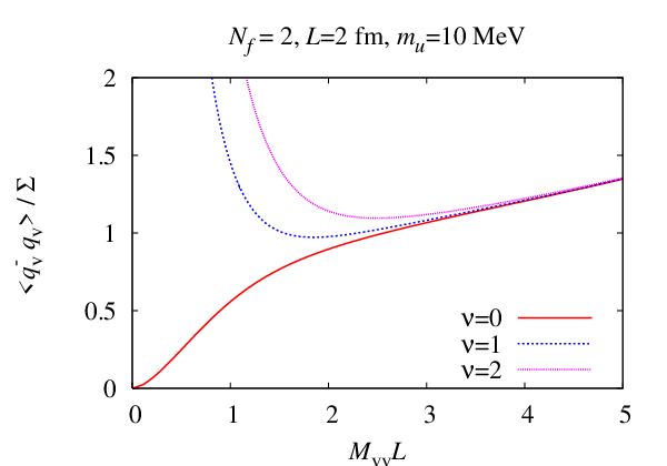
Substituting the explicit expressions above into Eq. (28) and (38), it is straightforward to compute numerically the chiral condensate and the spectral density of the Dirac operator. Using the numerical values listed in the beginning of this section, we plot the chiral condensate and the spectral density in Fig. 2 for the case of mu=md=m_{u}=m_{d}= 10 MeV, L=T/2=2L=T/2=2 fm, ν=0\nu=0 and here taking just as an example H2r​(0.77​GeV)=0.1×10⁻³H^{r}_{2}(0.77{\rm GeV})=0.1\times 10^{-3}. One sees that the resulting thick line smoothly connects the one in the ϵ\epsilon-regime (solid) with the one in the pp-regime (dotted)66 6 Because we do not have pp-regime predictions available at fixed topological charge ν\nu, we always compare with pp-regime expressions where topological sectors have been summed over. Of course, pp-regime predictions at fixed topology will differ slightly from these, but the difference becomes insignificant at large volumes.. It is clear that the effect of one-loop corrections to the spectral density of the Dirac operator in the pp-expansion is relatively small when Nf=2N_{f}=2, in agreement with the prediction Eq. (48) of Smilga and Stern [11].

It is useful to see what happens when we vary some parameters. In the larger volume (L=T/2=3L=T/2=3 fm) shown in Fig. 3 the agreement between the three different expansions becomes visibly better around M​L∼ML\sim2-3. The sea quark mass dependence is shown in Fig. 4 where we show the plots for different sea quark masses at 2 MeV (solid), 10 MeV (dotted), and 30 MeV (small dotted). The black filled circle in the left part shows the physical points where mv=mu=mdm_{v}=m_{u}=m_{d}. In Fig. 5 the ν\nu-dependence is presented at a fixed value of mu=10m_{u}=10 MeV and L=T/2=L=T/2= 2fm. The topology dependence disappears around Mv​v​L=3M_{vv}L=3-4. The condensate of the physical theory with mv=mu=mdm_{v}=m_{u}=m_{d} is plotted on the left part of Fig. 6 after summing of topology (See Appendix A for the details). Of course, the condensate in the massive case is inherently ambiguous due to the presence of the coupling H2H_{2}. On the other hand, the spectral density is free from this ambiguity. On the right part of Fig. 6 we plot the density after summing over topology at fixed mu=md=10m_{u}=m_{d}=10 MeV. As has been observed before [24], the striking oscillations that are seen at sectors of fixed topological charge become smeared out upon summing over topology. In the massless limit the oscillations will reappear and the density approaches that of the ν=0\nu=0 sector.

Refer to captionRefer to caption
Figure 2: The chiral condensate (top) and Dirac spectral density (bottom) for the case with mu=md=10m_{u}=m_{d}=10 MeV, L=T/2=2L=T/2=2 fm. The result of this paper is given by the thick line which smoothly connects the one in the ϵ\epsilon-regime (solid) with the on of pp-regime (dotted). Parameters have been chosen as Σ1/3=250\Sigma^{1/3}=250 MeV, F=90F=90 MeV, L6r​(μs​u​b=0.77​GeV)=0.05×10⁻³L^{r}_{6}(\mu_{sub}=0.77{\rm GeV})=0.05\times 10^{-3}, L8r​(μs​u​b=0.77​GeV)=0.5×10⁻³L^{r}_{8}(\mu_{sub}=0.77{\rm GeV})=0.5\times 10^{-3} and H2r​(μs​u​b=0.77​GeV)=0.1×10⁻³H^{r}_{2}(\mu_{sub}=0.77{\rm GeV})=0.1\times 10^{-3}.
Refer to captionRefer to caption
Figure 3: The same plots as in Fig. 2, the condensate (left) and the spectral density (right) but with the larger volume size L=T/2=3L=T/2=3 fm. The convergence of three expansions around Mv​v​L∼2M_{vv}L\sim 2-3 or λ​Σ​V∼\lambda\Sigma V\sim 10 becomes better.
Refer to captionRefer to caption
Figure 4: The condensate (left) and the spectral density (right) at fixed topology ν=0\nu=0 for different sea quark masses at 2 MeV (solid), 10 MeV (dotted), 30 MeV (small dotted) are given. We again set L=T/2=L=T/2= 2fm. The black filled circle in the left panel shows the physical points where mv=mu=mdm_{v}=m_{u}=m_{d}.
Refer to captionRefer to caption
Figure 5: The topology ν\nu dependence of the condensate (left) and the spectral density (right) at a fixed value of mu=10m_{u}=10 MeV and L=T/2=L=T/2= 2fm and H2r​(0.77​GeV)=0.1×10⁻³H^{r}_{2}(0.77{\rm GeV})=0.1\times 10^{-3}. The topology dependence becomes negligible around Mv​v​L=3M_{vv}L=3-4.
Refer to captionRefer to caption
Figure 6: The (full theory) condensate (left) where mv=mu=mdm_{v}=m_{u}=m_{d} and the spectral density (right) at fixed mu=md=10m_{u}=m_{d}=10 MeV, are given at θ=0\theta=0. Due to the ambiguity of H2rH_{2}^{r}, the condensate is not a well-defined quantity when MπM_{\pi} or Mv​v≠0M_{vv}\neq 0, while the spectral density is free from this ambiguity.

6.2 Nf=2+1N_{f}=2+1

Next, we consider the Nf=2+1N_{f}=2+1 theory where the strange quark mass is different from the up and down quark masses. Then G¯​(x,M2,M2)\bar{G}(x,M^{2},M^{2}) becomes much more complicated, and we refer to the explicit expressions given in Eqs. (D) and (43).

One obtains

Zv0\displaystyle Z^{0}_{v} =\displaystyle= 1−1F2[Mu​d216​π2lnMu​d22​μs​u​b2+2g¯1(Mu​d2/2)+Ms​s232​π2lnMs​s22​μs​u​b2+g¯1(Ms​s2/2)\displaystyle 1-\frac{1}{F^{2}}\left[\frac{M_{ud}^{2}}{16\pi^{2}}\ln\frac{M_{ud}^{2}}{2\mu_{sub}^{2}}+2\bar{g}_{1}\left(M_{ud}^{2}/2\right)+\frac{M_{ss}^{2}}{32\pi^{2}}\ln\frac{M_{ss}^{2}}{2\mu_{sub}^{2}}+\bar{g}_{1}\left(M_{ss}^{2}/2\right)\right. (74)
−13{−2​(Mu​d2−Ms​s2)2(Mu​d2+2​Ms​s2)2(Mu​d2+2​Ms​s23×16​π2lnMu​d2+2​Ms​s23​μs​u​b2+g¯1(Mu​d2+2​Ms​s23))\displaystyle\left.-\frac{1}{3}\left\{-\frac{2(M_{ud}^{2}-M_{ss}^{2})^{2}}{(M_{ud}^{2}+2M_{ss}^{2})^{2}}\left(\frac{M_{ud}^{2}+2M_{ss}^{2}}{3\times 16\pi^{2}}\ln\frac{M_{ud}^{2}+2M_{ss}^{2}}{3\mu_{sub}^{2}}+\bar{g}_{1}\left(\frac{M_{ud}^{2}+2M_{ss}^{2}}{3}\right)\right)\right.\right.
+(1+2​(Mu​d2−Ms​s2)2(Mu​d2+2​Ms​s2)2)(−β1V)−3​Mu​d2​Ms​s2Mu​d2+2​Ms​s2(−116​π2lnV1/2μs​u​b2−β2)}\displaystyle\left.\left.+\left(1+\frac{2(M_{ud}^{2}-M_{ss}^{2})^{2}}{(M_{ud}^{2}+2M_{ss}^{2})^{2}}\right)\left(-\frac{\beta_{1}}{\sqrt{V}}\right)-\frac{3M_{ud}^{2}M_{ss}^{2}}{M_{ud}^{2}+2M_{ss}^{2}}\left(-\frac{1}{16\pi^{2}}\ln V^{1/2}\mu_{sub}^{2}-\beta_{2}\right)\right\}\right.
−16L6r(μs​u​b)(2Mu​d2+Ms​s2)],\displaystyle\left.-16L^{r}_{6}(\mu_{sub})(2M_{ud}^{2}+M_{ss}^{2})\right],

and

δ​Zv​(mv)\displaystyle\delta Z_{v}(m_{v}) =\displaystyle= −1F2[Mu​d216​π2(1+mvmu)ln(1+mvmu)+Mu​d216​π2mvmulnMu​d22​μs​u​b2\displaystyle-\frac{1}{F^{2}}\left[\frac{M_{ud}^{2}}{16\pi^{2}}\left(1+\frac{m_{v}}{m_{u}}\right)\ln\left(1+\frac{m_{v}}{m_{u}}\right)+\frac{M_{ud}^{2}}{16\pi^{2}}\frac{m_{v}}{m_{u}}\ln\frac{M_{ud}^{2}}{2\mu_{sub}^{2}}\right. (75)
+2​g¯1​(Mu​d22​(1+mvmu))−2​g¯1​(Mu​d22)+Ms​s232​π2​(1+mvms)​ln⁡(1+mvms)\displaystyle\left.+2\bar{g}_{1}\left(\frac{M_{ud}^{2}}{2}\left(1+\frac{m_{v}}{m_{u}}\right)\right)-2\bar{g}_{1}\left(\frac{M_{ud}^{2}}{2}\right)+\frac{M_{ss}^{2}}{32\pi^{2}}\left(1+\frac{m_{v}}{m_{s}}\right)\ln\left(1+\frac{m_{v}}{m_{s}}\right)\right.
+Ms​s232​π2​mvms​ln⁡Ms​s22​μs​u​b2+g¯1​(Ms​s22​(1+mvms))−g¯1​(Ms​s22)\displaystyle\left.+\frac{M_{ss}^{2}}{32\pi^{2}}\frac{m_{v}}{m_{s}}\ln\frac{M_{ss}^{2}}{2\mu_{sub}^{2}}+\bar{g}_{1}\left(\frac{M_{ss}^{2}}{2}\left(1+\frac{m_{v}}{m_{s}}\right)\right)-\bar{g}_{1}\left(\frac{M_{ss}^{2}}{2}\right)\right.
−13{−2​(Mu​d2−Ms​s2)2(3​Mv​v2−Mu​d2−2​Ms​s2)2(Mu​d2+2​Ms​s23×16​π2lnMu​d2+2​Ms​s23​μs​u​b2+g¯1(Mu​d2+2​Ms​s23))\displaystyle\left.\hskip-36.135pt-\frac{1}{3}\left\{-\frac{2(M_{ud}^{2}-M_{ss}^{2})^{2}}{(3M_{vv}^{2}-M_{ud}^{2}-2M_{ss}^{2})^{2}}\left(\frac{M_{ud}^{2}+2M_{ss}^{2}}{3\times 16\pi^{2}}\ln\frac{M_{ud}^{2}+2M_{ss}^{2}}{3\mu_{sub}^{2}}+\bar{g}_{1}\left(\frac{M_{ud}^{2}+2M_{ss}^{2}}{3}\right)\right)\right.\right.
+(1+2​(Mu​d2−Ms​s2)2(3​Mv​v2−Mu​d2−2​Ms​s2)2)​(Mv​v216​π2​ln⁡Mv​v2μs​u​b2+g¯1​(Mv​v2))\displaystyle\left.\left.+\left(1+\frac{2(M_{ud}^{2}-M_{ss}^{2})^{2}}{(3M_{vv}^{2}-M_{ud}^{2}-2M_{ss}^{2})^{2}}\right)\left(\frac{M_{vv}^{2}}{16\pi^{2}}\ln\frac{M_{vv}^{2}}{\mu_{sub}^{2}}+\bar{g}_{1}(M_{vv}^{2})\right)\right.\right.
+3​(Mv​v2−Mu​d2)​(Mv​v2−Ms​s2)3​Mv​v2−Mu​d2−2​Ms​s2​(116​π2​(ln⁡Mv​v2μs​u​b2+1)+∂M2g¯1​(Mv​v2))\displaystyle\left.\left.+\frac{3(M_{vv}^{2}-M_{ud}^{2})(M_{vv}^{2}-M_{ss}^{2})}{3M_{vv}^{2}-M_{ud}^{2}-2M_{ss}^{2}}\left(\frac{1}{16\pi^{2}}(\ln\frac{M_{vv}^{2}}{\mu_{sub}^{2}}+1)+\partial_{M^{2}}\bar{g}_{1}(M_{vv}^{2})\right)\right.\right.
+2​(Mu​d2−Ms​s2)2(Mu​d2+2​Ms​s2)2​(Mu​d2+2​Ms​s23×16​π2​ln⁡Mu​d2+2​Ms​s23​μs​u​b2+g¯1​(Mu​d2+2​Ms​s23))\displaystyle\left.\left.+\frac{2(M_{ud}^{2}-M_{ss}^{2})^{2}}{(M_{ud}^{2}+2M_{ss}^{2})^{2}}\left(\frac{M_{ud}^{2}+2M_{ss}^{2}}{3\times 16\pi^{2}}\ln\frac{M_{ud}^{2}+2M_{ss}^{2}}{3\mu_{sub}^{2}}+\bar{g}_{1}\left(\frac{M_{ud}^{2}+2M_{ss}^{2}}{3}\right)\right)\right.\right.
−(1+2​(Mu​d2−Ms​s2)2(Mu​d2+2​Ms​s2)2)(−β1V)+3​Mu​d2​Ms​s2Mu​d2+2​Ms​s2(−116​π2lnV1/2μs​u​b2−β2)}\displaystyle\left.\left.\hskip-36.135pt-\left(1+\frac{2(M_{ud}^{2}-M_{ss}^{2})^{2}}{(M_{ud}^{2}+2M_{ss}^{2})^{2}}\right)\left(-\frac{\beta_{1}}{\sqrt{V}}\right)+\frac{3M_{ud}^{2}M_{ss}^{2}}{M_{ud}^{2}+2M_{ss}^{2}}\left(-\frac{1}{16\pi^{2}}\ln V^{1/2}\mu_{sub}^{2}-\beta_{2}\right)\right\}\right.
−4(2L8r(μs​u​b)+H2r(μs​u​b))Mv​v2],\displaystyle\left.-4(2L_{8}^{r}(\mu_{sub})+H_{2}^{r}(\mu_{sub}))M_{vv}^{2}\right],

where its real part for the imaginary valence mass is taken as in the same way shown in the previous subsection. Here Mu​d2=(mu+md)​Σ/F2,Ms​s2=2​ms​Σ/F2,Mv​v2=2​mv​Σ/F2M_{ud}^{2}=(m_{u}+m_{d})\Sigma/F^{2},M_{ss}^{2}=2m_{s}\Sigma/F^{2},M_{vv}^{2}=2m_{v}\Sigma/F^{2}.

The non-perturbative zero-mode integrals are given by

Σ^νPQ​(μv,{μu,μs})\displaystyle\hat{\Sigma}^{\rm PQ}_{\nu}(\mu_{v},\{\mu_{u},\mu_{s}\}) =\displaystyle= −1(μu2−μv2)2​(μs2−μv2)\displaystyle-\frac{1}{(\mu_{u}^{2}-\mu_{v}^{2})^{2}(\mu_{s}^{2}-\mu_{v}^{2})}
×det(∂μvKν​(μv)Iν​(μv)Iν​(μu)μu−1​Iν−1​(μu)Iν​(μs)−∂μv(μvKν+1(μv))μv​Iν+1​(μv)μu​Iν+1​(μu)Iν​(μu)μs​Iν+1​(μs)∂μv(μv2​Kν+2​(μv))μv2​Iν+2​(μv)μu2​Iν+2​(μu)μu​Iν+1​(μu)μs2​Iν+2​(μs)−∂μv(μv3Kν+3(μv))μv3​Iν+3​(μv)μu3​Iν+3​(μu)μu2​Iν+2​(μu)μs3​Iν+3​(μs)∂μv(μv4​Kν+4​(μv))μv4​Iν+4​(μv)μu4​Iν+4​(μu)μu3​Iν+3​(μu)μs4​Iν+4​(μs))det(Iν​(μu)μu−1​Iν−1​(μu)Iν​(μs)μu​Iν+1​(μu)Iν​(μu)μs​Iν+1​(μs)μu2​Iν+2​(μu)μu​Iν+1​(μu)μs2​Iν+2​(μs)).\displaystyle\hskip-72.26999pt\times\frac{\det\left(\begin{array}[]{ccccc}\partial_{\mu_{v}}K_{\nu}(\mu_{v})&I_{\nu}(\mu_{v})&I_{\nu}(\mu_{u})&\mu_{u}^{-1}I_{\nu-1}(\mu_{u})&I_{\nu}(\mu_{s})\\ -\partial_{\mu_{v}}(\mu_{v}K_{\nu+1}(\mu_{v}))&\mu_{v}I_{\nu+1}(\mu_{v})&\mu_{u}I_{\nu+1}(\mu_{u})&I_{\nu}(\mu_{u})&\mu_{s}I_{\nu+1}(\mu_{s})\\ \partial_{\mu_{v}}(\mu_{v}^{2}K_{\nu+2}(\mu_{v}))&\mu_{v}^{2}I_{\nu+2}(\mu_{v})&\mu_{u}^{2}I_{\nu+2}(\mu_{u})&\mu_{u}I_{\nu+1}(\mu_{u})&\mu_{s}^{2}I_{\nu+2}(\mu_{s})\\ -\partial_{\mu_{v}}(\mu_{v}^{3}K_{\nu+3}(\mu_{v}))&\mu_{v}^{3}I_{\nu+3}(\mu_{v})&\mu_{u}^{3}I_{\nu+3}(\mu_{u})&\mu_{u}^{2}I_{\nu+2}(\mu_{u})&\mu_{s}^{3}I_{\nu+3}(\mu_{s})\\ \partial_{\mu_{v}}(\mu_{v}^{4}K_{\nu+4}(\mu_{v}))&\mu_{v}^{4}I_{\nu+4}(\mu_{v})&\mu_{u}^{4}I_{\nu+4}(\mu_{u})&\mu_{u}^{3}I_{\nu+3}(\mu_{u})&\mu_{s}^{4}I_{\nu+4}(\mu_{s})\end{array}\right)}{\det\left(\begin{array}[]{ccc}I_{\nu}(\mu_{u})&\mu_{u}^{-1}I_{\nu-1}(\mu_{u})&I_{\nu}(\mu_{s})\\ \mu_{u}I_{\nu+1}(\mu_{u})&I_{\nu}(\mu_{u})&\mu_{s}I_{\nu+1}(\mu_{s})\\ \mu_{u}^{2}I_{\nu+2}(\mu_{u})&\mu_{u}I_{\nu+1}(\mu_{u})&\mu_{s}^{2}I_{\nu+2}(\mu_{s})\\ \end{array}\right)}.

where μu=mu,d​Σ​V\mu_{u}=m_{u,d}\Sigma V and μs=ms​Σ​V\mu_{s}=m_{s}\Sigma V and one can take the imaginary value of μv=i​ζ\mu_{v}=i\zeta to obtain ρ^νm​i​c​(ζ,{μu,μs})\hat{\rho}^{mic}_{\nu}(\zeta,\{\mu_{u},\mu_{s}\}) in the same way as the 2-flavor case.

Substituting again the numerical values in the beginning of this section, we plot the chiral condensate and the spectral density in Fig. 7 for the case with mu=md=m_{u}=m_{d}= 10 MeV, ms=110m_{s}=110 MeV, L=T/2=2L=T/2=2 fm, ν=0\nu=0 and H2r​(0.77​GeV)=0.1×10⁻³H^{r}_{2}(0.77{\rm GeV})=0.1\times 10^{-3}. Due to the large contribution from the chiral logarithm of strange quarks, both of the (normalized) condensate and spectral density shows a quite larger deviation from 1, which is the universal chiral limit when V→∞V\to\infty with any number of flavors.

Refer to captionRefer to caption
Figure 7: The condensate (top) and the Dirac spectral density (bottom) with Nf=2+1N_{f}=2+1 theory are given (solid curve). For the comparison, Nf=2N_{f}=2 plot is also presented (dotted). As the valence mass or the eigenvalue increases, both of them show larger deviation from 1 than the case with Nf=2N_{f}=2.

7 Conclusions

We have computed the quark condensate and the spectral density of the Dirac operator by means of the chiral Lagrangian in a finite volume. We have used a new perturbative method which keeps all the terms which appear in the conventional expansion in the pp-regime but which treats zero-mode integral non-perturbatively in the same manner as in the ϵ\epsilon-regime. The resulting perturbative series connects smoothly previous results in the pp-regime with those of the ϵ\epsilon-regime. Having analytical formulas available in the intermediate region may be of obvious value for lattice QCD simulations.

It would be interesting to investigate the present proposal for finite-volume chiral perturbation theory in greater detail. One should obviously consider using such a method to compute other finite-volume observables in chiral perturbation theory, such as two-point correlation functions.

Acknowledgments.
We thank Fabio Bernardoni, Shoji Hashimoto, Pilar Hernandez, Martin Lüscher and Kim Splittorff for discussions. The work of PHD was partly supported by the EU network ENRAGE MRTN-CT-2004-005616. The work of HF was supported by the Japanese Society for the Promotion of Science.

Appendix A Non-perturbative zero-mode integrals

In this appendix, we briefly review how to perform the non-perturbative zero-mode integrals. We are interested in the most general partially quenched calculations for both practical purposes of comparisons to lattice data and for computing spectral correlation functions of the Dirac operator. Of course, results for the NfN_{f}-theory without separate valence quarks are trivially included in this.

For the evaluation of the zero-mode integrals it is convenient to use the graded formalism where partial quenching is achieved by adding additional bosonic and fermionic species. The zero-mode integral corresponding to the graded version of Eq. (14) with nn bosons and mm fermions is known in closed analytical form for an arbitrary mass matrix [21],

𝒵n,mν​({μi})=det[μij−1𝒥ν+j−1(μi)]i,j=1,⋯n+m∏j>i=1n(μj2−μi2)​∏j>i=n+1n+m(μj2−μi2),\mathcal{Z}^{\nu}_{n,m}(\{\mu_{i}\})=\frac{\det[\mu_{i}^{j-1}\mathcal{J}_{\nu+j-1}(\mu_{i})]_{i,j=1,\cdots n+m}}{\prod_{j>i=1}^{n}(\mu_{j}^{2}-\mu_{i}^{2})\prod_{j>i=n+1}^{n+m}(\mu_{j}^{2}-\mu_{i}^{2})}, (1)

where μi=mi​Σ​V\mu_{i}=m_{i}\Sigma V. Here 𝒥\mathcal{J}’s are defined as 𝒥ν+j−1​(μi)≡(−1)j−1​Kν+j−1​(μi)\mathcal{J}_{\nu+j-1}(\mu_{i})\equiv(-1)^{j-1}K_{\nu+j-1}(\mu_{i}) for i=1,⋯ni=1,\cdots n and 𝒥ν+j−1​(μi)≡Iν+j−1​(μi)\mathcal{J}_{\nu+j-1}(\mu_{i})\equiv I_{\nu+j-1}(\mu_{i}) for i=n+1,⋯n+mi=n+1,\cdots n+m, where IνI_{\nu} and KνK_{\nu} are the modified Bessel functions. In this paper, we need the case with (n,m)=(1,Nf+1)(n,m)=(1,N_{f}+1):

𝒵1,1+Nfν​(μb|μv,{μs​e​a})\displaystyle\mathcal{Z}^{\nu}_{1,1+N_{f}}(\mu_{b}|\mu_{v},\{\mu_{sea}\}) =\displaystyle= 1∏i=1Nf(μi2−μv2)​∏j>kNf(μj2−μk2)\displaystyle\frac{1}{\prod_{i=1}^{N_{f}}(\mu_{i}^{2}-\mu_{v}^{2})\prod_{j>k}^{N_{f}}(\mu_{j}^{2}-\mu_{k}^{2})}
×det(Kν​(μb)Iν​(μv)Iν​(μ1)Iν​(μ2)⋯−μb​Kν+1​(μb)μv​Iν+1​(μv)μ1​Iν+1​(μ1)μ2​Iν+1​(μ2)⋯μb2​Kν+2​(μb)μv2​Iν+2​(μv)μ12​Iν+2​(μ1)μ22​Iν+2​(μ2)⋯⋯⋯⋯⋯⋯).\displaystyle\hskip-72.26999pt\times\det\left(\begin{array}[]{ccccc}K_{\nu}(\mu_{b})&I_{\nu}(\mu_{v})&I_{\nu}(\mu_{1})&I_{\nu}(\mu_{2})&\cdots\\ -\mu_{b}K_{\nu+1}(\mu_{b})&\mu_{v}I_{\nu+1}(\mu_{v})&\mu_{1}I_{\nu+1}(\mu_{1})&\mu_{2}I_{\nu+1}(\mu_{2})&\cdots\\ \mu_{b}^{2}K_{\nu+2}(\mu_{b})&\mu_{v}^{2}I_{\nu+2}(\mu_{v})&\mu_{1}^{2}I_{\nu+2}(\mu_{1})&\mu^{2}_{2}I_{\nu+2}(\mu_{2})&\cdots\\ \cdots&\cdots&\cdots&\cdots&\cdots\end{array}\right).

Here μb=mb​Σ​V\mu_{b}=m_{b}\Sigma V, μv=mv​Σ​V\mu_{v}=m_{v}\Sigma V and μi=mi​Σ​V\mu_{i}=m_{i}\Sigma V, where mbm_{b}, mvm_{v} and mim_{i} denote the masses of the valence bosons, the valence quarks, and the physical sea quarks respectively. In the arguments, the set of sea flavors are denoted by {μs​e​a}={m1​Σ​V,m2​Σ​V,⋯}\{\mu_{sea}\}=\{m_{1}\Sigma V,m_{2}\Sigma V,\cdots\}.

When some of the quark masses are degenerate, one simply uses l’Hopital’s rule. For example, for μ1=μ2\mu_{1}=\mu_{2} one has

𝒵1,1+Nfν​(μb|μv,{μs​e​a})|μ1=μ2\displaystyle\mathcal{Z}^{\nu}_{1,1+N_{f}}(\mu_{b}|\mu_{v},\{\mu_{sea}\})|_{\mu_{1}=\mu_{2}} =\displaystyle= 12​∏i=1Nf(μi2−μv2)​∏j>k,j≥3Nf(μj2−μk2)\displaystyle\frac{1}{2\prod_{i=1}^{N_{f}}(\mu_{i}^{2}-\mu_{v}^{2})\prod_{j>k,j\geq 3}^{N_{f}}(\mu_{j}^{2}-\mu_{k}^{2})}
×det(Kν​(μb)Iν​(μv)Iν​(μ1)μ1−1​Iν−1​(μ1)⋯−μb​Kν+1​(μb)μv​Iν+1​(μv)μ1​Iν+1​(μ1)Iν​(μ1)⋯μb2​Kν+2​(μb)μv2​Iν+2​(μv)μ12​Iν+2​(μ1)μ1​Iν+1​(μ1)⋯⋯⋯⋯⋯⋯).\displaystyle\hskip-108.405pt\times\det\left(\begin{array}[]{ccccc}K_{\nu}(\mu_{b})&I_{\nu}(\mu_{v})&I_{\nu}(\mu_{1})&\mu_{1}^{-1}I_{\nu-1}(\mu_{1})&\cdots\\ -\mu_{b}K_{\nu+1}(\mu_{b})&\mu_{v}I_{\nu+1}(\mu_{v})&\mu_{1}I_{\nu+1}(\mu_{1})&I_{\nu}(\mu_{1})&\cdots\\ \mu_{b}^{2}K_{\nu+2}(\mu_{b})&\mu_{v}^{2}I_{\nu+2}(\mu_{v})&\mu_{1}^{2}I_{\nu+2}(\mu_{1})&\mu_{1}I_{\nu+1}(\mu_{1})&\cdots\\ \cdots&\cdots&\cdots&\cdots&\cdots\end{array}\right).

Partially quenched observables are computed by differentiating Eq. (A) with respect to suitable sources and subsequently taking the limit μb→μv\mu_{b}\to\mu_{v}. For example, the zero-mode integral of Eq. (15) is

12⟨Uv​v+Uv​v†⟩U=Σ^νPQ(μv,{μs​e​a})≡−limμb→μv∂∂μbln𝒵1,1+Nfν(μb|μv,{μs​e​a}).\displaystyle\frac{1}{2}\langle U_{vv}+U^{\dagger}_{vv}\rangle_{U}=\hat{\Sigma}^{\rm PQ}_{\nu}(\mu_{v},\{\mu_{sea}\})\equiv-\lim_{\mu_{b}\to\mu_{v}}\frac{\partial}{\partial\mu_{b}}\ln\mathcal{Z}^{\nu}_{1,1+N_{f}}(\mu_{b}|\mu_{v},\{\mu_{sea}\}). (12)

To obtain the result in a θ=0\theta=0 (or even θ≠0\theta\neq 0) QCD vacuum, one could numerically sum over topology with the weight given by the partition function above;

Σ^θPQ​(μv,{μs​e​a})\displaystyle\hat{\Sigma}_{\theta}^{\rm PQ}(\mu_{v},\{\mu_{sea}\}) =\displaystyle= ∑νei​θ​ν​Σ^νPQ​(μv,{μs​e​a})​𝒵0,Nfν∑νei​θ​ν​𝒵0,Nfν,\displaystyle\frac{\sum_{\nu}e^{i\theta\nu}\hat{\Sigma}_{\nu}^{\rm PQ}(\mu_{v},\{\mu_{sea}\})\mathcal{Z}^{\nu}_{0,N_{f}}}{\sum_{\nu}e^{i\theta\nu}\mathcal{Z}^{\nu}_{0,N_{f}}}, (13)

or use the analytic expressions known for the Nf=2,3N_{f}=2,3 cases [25].

Appendix B Doing the zero-mode integrals first: a U⁡(1)U(1) toy model

The perturbative scheme presented in this paper relies on the operator

Σ2​F2​[ℳ†​(U−1)​ξ2+ξ2​(U†−1)​ℳ],\frac{\Sigma}{2F^{2}}[\mathcal{M}^{\dagger}(U-1)\xi^{2}+\xi^{2}(U^{\dagger}-1)\mathcal{M}],

being small, and more precisely of 𝒪⁡(p5){\cal O}(p^{5}) or smaller, for any value of the mass mm as this mass is taken to zero at finite volume. The difficulty in giving a precise counting to this term lies of course in it being a combination of mass mm, field ξ⁡(x)\xi(x) (both of which can be assigned clear countings) and the zero mode field UU. It is therefore interesting that an alternative scheme exists, which gives identical results, but which assigns a definite magnitude to this term. This is achieved by first doing the zero mode integral exactly, and only subsequently performing the perturbative evaluations of the non-zero mode integrals77 7 We are grateful to M. Lüscher for suggesting this alternative method.. In the general S​U​(Nf+N)SU(N_{f}+N) case this becomes rather cumbersome in practice, but it has the advantage that all terms are explicitly ordered according to the expansion parameter 1/L1/L. Here we illustrate it for the case of a simple U⁡(1)U(1) toy model at the topological sector with ν=0\nu=0, where the zero-mode integrals are trivially performed.

We thus consider the U⁡(1)U(1) ‘‘chiral Lagrangian’’88 8 Of course, in the real Nf=1N_{f}=1 theory chiral symmetry is broken explicitly by the anomaly, and this Lagrangian is therefore not relevant for describing the the Nf=1N_{f}=1 theory. We use it only as a simple toy model to illustrate in a very transparent way the effect of first integrating over the zero mode.

ℒ=F24∂μU(x)∂μU†(x)−Σ2[m†ei​θU(x)+h.c.]+⋯,{\cal L}~=~\frac{F^{2}}{4}\partial_{\mu}U(x)\partial_{\mu}U^{\dagger}(x)-\frac{\Sigma}{2}[m^{\dagger}e^{i\theta}U(x)+{\rm h.c.}]+\cdots, (1)

where U⁡(x)∈U⁡(1)U(x)\in U(1). We separate into zero modes and non-zero modes,

U⁡(x)=U​ei​2​ξ​(x)/F=ei​2​ξ0/F​ei​2​ξ​(x)/F,U(x)~=~Ue^{i\sqrt{2}\xi(x)/F}~=~e^{i\sqrt{2}\xi_{0}/F}e^{i\sqrt{2}\xi(x)/F}, (2)

and do the analogue of fixing topology to ν=0\nu=0 by integrating over θ\theta. Expanding perturbatively in the non-zero modes ξ⁡(x)\xi(x), we get

ℒ=−Σ​m​cos⁡(2​ξ0/F)​(1−ξ​(x)2/F2)+12​(∂μξ⁡(x))2+⋯,\displaystyle{\cal L}=-\Sigma m\cos(\sqrt{2}\xi_{0}/F)\left(1-\xi(x)^{2}/F^{2}\right)+\frac{1}{2}(\partial_{\mu}\xi(x))^{2}+\cdots, (3)

We now perform the zero-mode integration over ξ0\xi_{0} exactly with respect to the term shown to get the partition function

𝒵=∫[dξ(x)]I0(mΣV(1−1V​F2∫d4xξ(x)2))e−12∫d4x(∂μξ)2+⋯,\displaystyle{\cal Z}=\int[d\xi(x)]I_{0}\left(m\Sigma V\left(1-\frac{1}{VF^{2}}\int d^{4}x\xi(x)^{2}\right)\right)e^{-\frac{1}{2}\int d^{4}x(\partial_{\mu}\xi)^{2}}+\cdots, (4)

up to overall irrelevant factors.

Expanding the Bessel function using I0′​(x)=I1​(x)I_{0}^{\prime}(x)=I_{1}(x), and exponentiating the expanded term leads to the effective partition function

𝒵=I0(mΣV)∫[dξ(x)]e−∫d4x[12(∂μξ)2+12m~π2ξ(x)2]+⋯,\displaystyle{\cal Z}=I_{0}(m\Sigma V)\int[d\xi(x)]e^{-\int d^{4}x[\frac{1}{2}(\partial_{\mu}\xi)^{2}+\frac{1}{2}\tilde{m}_{\pi}^{2}\xi(x)^{2}]}+\cdots, (5)

where an effective volume-dependent pion mass is defined by

m~π2≡2​m​ΣF2​I1​(m​Σ​V)I0​(m​Σ​V),\tilde{m}_{\pi}^{2}~\equiv~\frac{2m\Sigma}{F^{2}}~\frac{I_{1}(m\Sigma V)}{I_{0}(m\Sigma V)}, (6)

we note that, as expected, this effective pion mass approaches the standard tree-level pion mass expression in the limit where m​Σ​V→∞m\Sigma V\to\infty:

m~π2→2​m​Σ/F2=mπ2as​m​Σ​V→∞,\tilde{m}_{\pi}^{2}~\to~2m\Sigma/F^{2}=m_{\pi}^{2}~~~~~~~~{\rm as}~~m\Sigma V\to\infty, (7)

while in the opposite limit we find

m~π2∼2​m​ΣF2​12​m​Σ​V=mπ4​F2​V4as​m​Σ​V→0,\tilde{m}_{\pi}^{2}~\sim~\frac{2m\Sigma}{F^{2}}~\frac{1}{2}m\Sigma V=m_{\pi}^{4}~\frac{F^{2}V}{4}~~~~~~~~{\rm as}~~m\Sigma V\to 0, (8)

Clearly, in the usual pp-regime expansion this provides us with the standard massive propagator term, while in the chiral limit taken at finite volume VV, there is no infrared problem due to the momentum sums being taken over non-zero modes only. When m​Σ​Vm\Sigma V becomes of order unity we recover the usual ϵ\epsilon-regime expressions.

But here we are interested in seeing how our expansion looks if we add and subtract the standard mass term, as is done in the main part of this paper. We therefore do a trivial rewriting,

ℒ\displaystyle{\cal L} =\displaystyle= 12​(∂μξ⁡(x))2+12​m~π2​ξ​(x)2\displaystyle\frac{1}{2}(\partial_{\mu}\xi(x))^{2}+\frac{1}{2}\tilde{m}_{\pi}^{2}\xi(x)^{2} (9)
=\displaystyle= 12​(∂μξ⁡(x))2+12​mπ2​ξ​(x)2+12​δ​mπ2​ξ​(x)2,\displaystyle\frac{1}{2}(\partial_{\mu}\xi(x))^{2}+\frac{1}{2}m_{\pi}^{2}\xi(x)^{2}+\frac{1}{2}\delta m_{\pi}^{2}\xi(x)^{2}, (10)

where

δ​mπ2≡m~π2−mπ2,\delta m_{\pi}^{2}~\equiv~\tilde{m}_{\pi}^{2}-m_{\pi}^{2}, (11)

Can we treat 12​δ​mπ2​ξ​(x)2\frac{1}{2}\delta m_{\pi}^{2}\xi(x)^{2} as a perturbation? Near the usual pp-regime where m​Σ​V→∞m\Sigma V\to\infty we can use the asymptotic expansion of Bessel functions,

In​(x)∼ex2​π​x​(1−4​n2−18​x+⋯),I_{n}(x)\sim\frac{e^{x}}{\sqrt{2\pi x}}\left(1-\frac{4n^{2}-1}{8x}+\cdots\right), (12)

to see that

δ​mπ2=−1F2​V+⋯,\delta m_{\pi}^{2}=-\frac{1}{F^{2}V}+\cdots, (13)

This is of 𝒪⁡(p4){\cal O}(p^{4}) as expected in this U⁡(1)U(1) theory. When instead m​Σ​Vm\Sigma V is of order unity, we get

δ​mπ2∼−mπ2,\delta m_{\pi}^{2}\sim-m_{\pi}^{2}, (14)

which is also of 𝒪⁡(p4){\cal O}(p^{4}). The point here is that we know the full analytical expression

δ​mπ2=2​m​ΣF2​[I1​(m​Σ​V)I0​(m​Σ​V)−1],\delta m_{\pi}^{2}~=~\frac{2m\Sigma}{F^{2}}\left[\frac{I_{1}(m\Sigma V)}{I_{0}(m\Sigma V)}-1\right], (15)

for all values of mm and VV, and it is easy to check that this function is of 𝒪⁡(p4){\cal O}(p^{4}) everywhere. The term δ​mπ2​ξ​(x)2\delta m_{\pi}^{2}\xi(x)^{2} is thus explicitly found to be of NLO and we can treat it perturbatively.

Of course, as already discussed in Section 5, away from the conventional pp-regime expansion, separating out δ​mπ2​ξ​(x)2\delta m_{\pi}^{2}\xi(x)^{2} and treating it perturbatively amounts to a re-ordering and partial resummation of terms in this expansion. This is because the propagator is taken to be the conventional massive one even when mπ2m_{\pi}^{2} is no longer of 𝒪⁡(p2){\cal O}(p^{2}), but smaller. The difference between a calculation based on this propagator and one where the propagator has been expanded in mπ2m_{\pi}^{2} up to the needed order is always of yet higher order, and thus only illustrates the inherent uncertainty in any fixed-order perturbative expansion.

Appendix C Numerical evaluation of Δ¯​(0,M2)\bar{\Delta}(0,M^{2}) and ∂M2Δ¯​(0,M2)\partial_{M^{2}}\bar{\Delta}(0,M^{2})

The definition of g¯1​(M2)\bar{g}_{1}(M^{2}) in Eq. (20) and g¯2(M2)=−∂M2g¯1(M2)\bar{g}_{2}(M^{2})=-\partial_{M^{2}}\bar{g}_{1}(M^{2}), requires an infinite sum over the 4-vector aμ=nμ​Lμa_{\mu}=n_{\mu}L_{\mu} where Li=L⁡(i=1,2,3)L_{i}=L\;(i=1,2,3) and L4=TL_{4}=T. In this appendix, we will suggest how to evaluate numerically g¯1​(M2)\bar{g}_{1}(M^{2}) and g¯2​(M2)\bar{g}_{2}(M^{2}).

For M​L>1ML>1, the expansion [6],

g¯1​(M2)=∑a≠0∫d4​q(2​π)4​e−i​q​aq2+M2−1M2​V=∑a≠0M24​π2​|a|​K1​(M2​|a|)−1M2​V,\displaystyle\bar{g}_{1}(M^{2})=\sum_{a\neq 0}\int\frac{d^{4}q}{(2\pi)^{4}}\frac{e^{-iqa}}{q^{2}+M^{2}}-\frac{1}{M^{2}V}=\sum_{a\neq 0}\frac{\sqrt{M^{2}}}{4\pi^{2}|a|}K_{1}(\sqrt{M^{2}}|a|)-\frac{1}{M^{2}V}, (16)

in terms of modified Bessel functions is useful, while for M​L<1ML<1, the polynomial expression

g¯1​(M2)=−M216​π2​ln⁡(M2​V1/2)−∑n=1∞βn(n−1)!​M2​(n−1)​V(n−2)/2,\displaystyle\bar{g}_{1}(M^{2})=-\frac{M^{2}}{16\pi^{2}}\ln(M^{2}V^{1/2})-\sum^{\infty}_{n=1}\frac{\beta_{n}}{(n-1)!}M^{2(n-1)}V^{(n-2)/2}, (17)

using the shape coefficients βn\beta_{n}’s [4] is appropriate. Here

βn\displaystyle\beta_{n} ≡\displaystyle\equiv (−14​π)n​(αn+2n⁡(n−2))​(n≠2),β2≡α2−ln⁡4​π+γ−3/216​π2,\displaystyle\left(\frac{-1}{4\pi}\right)^{n}\left(\alpha_{n}+\frac{2}{n(n-2)}\right)\;\;\;(n\neq 2),\;\;\;\;\;\beta_{2}\equiv\frac{\alpha_{2}-\ln 4\pi+\gamma-3/2}{16\pi^{2}}, (18)
αn\displaystyle\alpha_{n} ≡\displaystyle\equiv ∫01dt{tn−3(S(L2V1/2​t)3S(T2V1/2​t)−1)\displaystyle\int_{0}^{1}dt\left\{t^{n-3}\left(S\left(\frac{L^{2}}{V^{1/2}t}\right)^{3}S\left(\frac{T^{2}}{V^{1/2}t}\right)-1\right)\right. (19)
+t−n−1(S(V1/2L2​t)3S(V1/2T2​t)−1)},\displaystyle\left.\hskip 72.26999pt+t^{-n-1}\left(S\left(\frac{V^{1/2}}{L^{2}t}\right)^{3}S\left(\frac{V^{1/2}}{T^{2}t}\right)-1\right)\right\},
S⁡(x)\displaystyle S(x) ≡\displaystyle\equiv ∑k=−∞∞exp⁡(−π​k2​x),\displaystyle\sum^{\infty}_{k=-\infty}\exp(-\pi k^{2}x), (20)

where γ∼0.577215665\gamma\sim 0.577215665 is Euler’s constant and the summation in S⁡(x)S(x) is typically well approximated by a truncation to |k|≤20|k|\leq 20.

Since the modified Bessel function Kν​(x)K_{\nu}(x) is well-defined for the complex value of xx, the both expressions above can be easily extended for the complex arguments using (m+mv2)1/2|mv=i​λ=(m2+λ2)1/4​ei​arctan⁡(λ/m)/2(m+\sqrt{m_{v}^{2}})^{1/2}|_{m_{v}=i\lambda}=(m^{2}+\lambda^{2})^{1/4}e^{i\arctan(\lambda/m)/2}, and the prescription given in Eq. (32).

As shown in Fig. 8, ignoring the contribution from |nμ|>20|n_{\mu}|>20 in the summation in Eq. (16), and n>5n>5 in the summation in Eq. (17), both formulas agree in a rather long interval around M​L=1ML=1. We also find an excellent agreement between these two expansions for both Re​g¯1​(M2){\rm Re}\bar{g}_{1}(M^{2}) and Re​g¯2​(M2){\rm Re}\bar{g}_{2}(M^{2}) at imaginary values of M2M^{2}, using the same truncation. It is in any case trivial to increase the accuracy by including more terms.

To summarize, we have used

g¯1​(M2)={g¯1p​(M2)≡∑a≠0|ni|≤20M24​π2​|a|​K1​(M2​|a|)−1M2​V(|M|​L>1)g¯1ϵ​(M2)≡−M216​π2​ln⁡(M2​V1/2)−∑n=15βn(n−1)!​M2​(n−1)​V(n−2)/2(|M|​L≤1),\displaystyle\bar{g}_{1}(M^{2})=\left\{\begin{array}[]{lc}\bar{g}^{p}_{1}(M^{2})\equiv\sum_{a\neq 0}^{|n_{i}|\leq 20}\frac{\sqrt{M^{2}}}{4\pi^{2}|a|}K_{1}(\sqrt{M^{2}}|a|)-\frac{1}{M^{2}V}&(|M|L>1)\\ \\ \bar{g}^{\epsilon}_{1}(M^{2})\equiv-\frac{M^{2}}{16\pi^{2}}\ln(M^{2}V^{1/2})-\sum^{5}_{n=1}\frac{\beta_{n}}{(n-1)!}M^{2(n-1)}V^{(n-2)/2}&(|M|L\leq 1)\end{array}\right.,

and similarly for their derivatives g¯2\bar{g}_{2}. We plot R​e​g¯1​(M02+i​M2){Re}\bar{g}_{1}(M^{2}_{0}+iM^{2}) and R​e​g¯2​(M02+i​M2){Re}\bar{g}_{2}(M^{2}_{0}+iM^{2}) for various choices of fixed M0M_{0} in Fig. 9.

Specifying the renormalization scale μs​u​b=0.77\mu_{sub}=0.77 GeV of the low energy constants LiL_{i}’s, and the above prescription for g¯1\bar{g}_{1} and g¯2\bar{g}_{2},

Δ¯​(0,M2)\displaystyle\bar{\Delta}(0,M^{2}) =\displaystyle= M216​π2​ln⁡M2μs​u​b2+g¯1​(M2),\displaystyle\frac{M^{2}}{16\pi^{2}}\ln\frac{M^{2}}{\mu_{sub}^{2}}+\bar{g}_{1}(M^{2}), (26)
∂M2Δ¯​(0,M2)\displaystyle\partial_{M^{2}}\bar{\Delta}(0,M^{2}) =\displaystyle= 116​π2​(ln⁡M2μs​u​b2+1)−g¯2​(M2),\displaystyle\frac{1}{16\pi^{2}}\left(\ln\frac{M^{2}}{\mu_{sub}^{2}}+1\right)-\bar{g}_{2}(M^{2}), (27)

can then be evaluated numerically. We note that in the small mass region the logarithmic contribution ln⁡M2\ln M^{2} is canceled by a similar one in g¯i\bar{g}_{i} and that both Δ¯​(0,M2)\bar{\Delta}(0,M^{2}) and ∂M2Δ¯​(0,M2)\partial_{M^{2}}\bar{\Delta}(0,M^{2}) have no IR divergences in the limit M2→0M^{2}\to 0.

Refer to captionRefer to caption
Figure 8: The plot of g¯1​(M2)​V1/2\bar{g}_{1}(M^{2})V^{1/2} (left part) and g¯2​(M2)\bar{g}_{2}(M^{2}) (right part) for T=2​LT=2L. The truncated sums in Eq. (C) for g¯1,2p​(M2)\bar{g}^{p}_{1,2}(M^{2}) (solid line) and g¯1,2ϵ​(M2)\bar{g}^{\epsilon}_{1,2}(M^{2}) (dotted) agree well around M​L∼1ML\sim 1. Note that g¯1​(M2)​V1/2\bar{g}_{1}(M^{2})V^{1/2} converges to −β1=−0.08360-\beta_{1}=-0.08360 in the chiral limit. Note also that |g¯1​(M2)||\bar{g}_{1}(M^{2})| attains its maximum at M=0M=0.
Refer to captionRefer to caption
Figure 9: Plot of Re​g¯1​(M02+i​M2)​V1/2{\rm Re}\bar{g}_{1}(M^{2}_{0}+iM^{2})V^{1/2} (left part) and Re​g¯2​(M02+i​M2){\rm Re}\bar{g}_{2}(M^{2}_{0}+iM^{2}) (right part) for T=2​LT=2L. for three fixed values of M0​L=0M_{0}L=0 (solid), 0.05 (dotted) and 0.1 (small dotted).

Appendix D Useful properties of G¯​(x,M2,M2)\bar{G}(x,M^{2},M^{2})

We also need the 1-loop correction from off-diagonals part of ξ\xi, G¯​(0,M2,M2)\bar{G}(0,M^{2},M^{2}). It can, in principle, be expressed in terms of Δ¯​(0,M2)\bar{\Delta}(0,M^{2}). In this appendix, we discuss the UV divergence of G¯​(0,M2,M2)\bar{G}(0,M^{2},M^{2}) and rewrite it using Δ¯​(0,M2)\bar{\Delta}(0,M^{2}) and ∂M2Δ¯​(0,M2)\partial_{M^{2}}\bar{\Delta}(0,M^{2}). Explicit examples for the degenerate case and non-degenerate Nf=2+1N_{f}=2+1 flavor theory will be given.

First let us consider the UV-divergent part of Δ¯​(0,M2)\bar{\Delta}(0,M^{2}),

Δ¯​(0,M2)\displaystyle\bar{\Delta}(0,M^{2}) =\displaystyle= 1V​∑p≠01p2+M2\displaystyle\frac{1}{V}\sum_{p\neq 0}\frac{1}{p^{2}+M^{2}} (28)
=\displaystyle= 1V​∑p≠0(1p2−M2p4)+𝒪⁡(M4).\displaystyle\frac{1}{V}\sum_{p\neq 0}\left(\frac{1}{p^{2}}-\frac{M^{2}}{p^{4}}\right)+{\cal O}(M^{4}).

Here the first term is quadratically divergent, the second term produces a logarithmic divergence, and the remaining 𝒪⁡(M4){\cal O}(M^{4}) terms are UV finite. As is well-known. the quadratic divergence is absent when we employ dimensional regularization.

By expanding in the mass, the UV-divergent part of G¯​(0,M2,M2)\bar{G}(0,M^{2},M^{2}) can be written

G¯​(0,M2,M2)\displaystyle\bar{G}(0,M^{2},M^{2}) =\displaystyle= 1V​∑p≠01(p2+M2)2​(∑fNf1p2+Mf​f2)\displaystyle\frac{1}{V}\sum_{p\neq 0}\frac{1}{(p^{2}+M^{2})^{2}\left(\sum_{f}^{N_{f}}\frac{1}{p^{2}+M^{2}_{ff}}\right)} (29)
=\displaystyle= 1Nf​V​∑p≠0(1p2−2​M2p4+1Nf​∑fNfMf​f2p4+𝒪⁡(M4))\displaystyle\frac{1}{N_{f}V}\sum_{p\neq 0}\left(\frac{1}{p^{2}}-\frac{2M^{2}}{p^{4}}+\frac{1}{N_{f}}\sum^{N_{f}}_{f}\frac{M^{2}_{ff}}{p^{4}}+{\cal O}(M^{4})\right)
=\displaystyle= 2Nf​Δ¯​(0,M2)−1Nf2​∑fNfΔ¯​(0,Mf​f2)+𝒪⁡(M4)\displaystyle\frac{2}{N_{f}}\bar{\Delta}(0,M^{2})-\frac{1}{N_{f}^{2}}\sum^{N_{f}}_{f}\bar{\Delta}(0,M^{2}_{ff})+{\cal O}(M^{4})
=\displaystyle= (2Nf​M2−1Nf2​∑fNfMf​f2)​c116​π2+⋯,\displaystyle\left(\frac{2}{N_{f}}M^{2}-\frac{1}{N_{f}^{2}}\sum^{N_{f}}_{f}M^{2}_{ff}\right)\frac{c_{1}}{16\pi^{2}}+\cdots,

where the logarithmic divergence of the last line is canceled by a renormalization of LiL_{i}’s as seen in Section 3.

Although Eq. (29) shows that G¯​(0,M2,M2)\bar{G}(0,M^{2},M^{2}) inherits the UV properties of Δ¯​(0,M2)\bar{\Delta}(0,M^{2}), the expansion is not useful when we want to see the finite part of G¯​(0,M2,M2)\bar{G}(0,M^{2},M^{2}), since the omitted 𝒪⁡(M4){\cal O}(M^{4}) terms are the at the same order as the former two terms. In order to obtain a convenient rewriting, let us define a function

f⁡(t)≡1Nf​∑iknit−Mi​i2,\displaystyle f(t)\equiv\frac{1}{N_{f}}\sum^{k}_{i}\frac{n_{i}}{t-M^{2}_{ii}}, (30)

where kk denotes the number of different quark masses and ni≥1n_{i}\geq 1 is the degeneracy of the ii-th mass satisfying ∑ikni=Nf\sum^{k}_{i}n_{i}=N_{f}. Here we have ordered the masses Mi​i2<Mi+1​i+12M^{2}_{ii}<M^{2}_{i+1\;i+1} for any ii. Noting f⁡(t)f(t) is a monotonically decreasing function,

dd​tf(t)=−1Nf∑ikni(t−Mi​i2)2<0,\displaystyle\frac{d}{dt}f(t)=-\frac{1}{N_{f}}\sum^{k}_{i}\frac{n_{i}}{(t-M^{2}_{ii})^{2}}<0, (31)

and

limϵ→0f⁡(Mi​i2+ϵ)\displaystyle\lim_{\epsilon\to 0}f(M_{ii}^{2}+\epsilon) =\displaystyle= ∞,limϵ→0f⁡(Mi+1​i+12−ϵ)=−∞,\displaystyle\infty,\;\;\;\lim_{\epsilon\to 0}f(M_{i+1\;i+1}^{2}-\epsilon)=-\infty, (32)
f⁡(t)\displaystyle f(t) ≠\displaystyle\neq 0,for​t<M112,Mk​k2<t,\displaystyle 0,\;\;\;\mbox{for}\;\;\;t<M^{2}_{11},M^{2}_{kk}<t, (33)

one can show that an equation f⁡(t)=0f(t)=0 has k−1k-1 different solutions (we denote them by t=M¯i​i2t=\bar{M}^{2}_{ii}), each of them satisfying

Mi​i2<M¯i​i2<Mi+1​i+12,(1≤i≤k−1).\displaystyle M^{2}_{ii}<\bar{M}^{2}_{ii}<M^{2}_{i+1\;i+1},\;\;\;(1\leq i\leq k-1). (34)

We illustrate this in the plot Fig. 10.

Hence,

−f⁡(−p2)=∏ik−1(p2+M¯i​i2)∏jk(p2+Mj​j2),\displaystyle-f(-p^{2})=\frac{\prod_{i}^{k-1}(p^{2}+\bar{M}^{2}_{ii})}{\prod_{j}^{k}(p^{2}+M^{2}_{jj})}, (35)

and G¯​(0,M2,M2)\bar{G}(0,M^{2},M^{2}) can thus alternatively be expressed as

G¯​(0,M2,M2)\displaystyle\bar{G}(0,M^{2},M^{2}) =\displaystyle= 1Nf​V​∑p≠0∏jk(p2+Mj​j2)(p2+M2)2​∏ik−1(p2+M¯i​i2)\displaystyle\frac{1}{N_{f}V}\sum_{p\neq 0}\frac{\prod_{j}^{k}(p^{2}+M^{2}_{jj})}{(p^{2}+M^{2})^{2}\prod_{i}^{k-1}(p^{2}+\bar{M}^{2}_{ii})} (36)
=\displaystyle= 1Nf​[∑ik−1Ai​Δ¯​(0,M¯i​i2)+B​Δ¯​(0,M2)+C​∂M2Δ¯​(0,M2)],\displaystyle\frac{1}{N_{f}}\left[\sum^{k-1}_{i}A_{i}\bar{\Delta}(0,\bar{M}^{2}_{ii})+B\bar{\Delta}(0,M^{2})+C\;\partial_{M^{2}}\bar{\Delta}(0,M^{2})\right],

where the coefficients AiA_{i}’s, BB and CC are given by the residue of

f2​(t)=∏jk(−t+Mj​j2)(−t+M2)2​∏ik−1(−t+M¯i​i2),\displaystyle f_{2}(t)=\frac{\prod_{j}^{k}(-t+M^{2}_{jj})}{(-t+M^{2})^{2}\prod_{i}^{k-1}(-t+\bar{M}^{2}_{ii})}, (37)

(or −(−t+M2)​f2​(t)-(-t+M^{2})f_{2}(t) for CC), at each pole. Note that C=0C=0 when M2M^{2} is equal to any of the physical masses.

Noting that both Δ¯​(0,M2)\bar{\Delta}(0,M^{2}) and ∂M2Δ¯​(0,M2)\partial_{M^{2}}\bar{\Delta}(0,M^{2}) are infra-red finite in the limit M2→0M^{2}\to 0,

Δ¯​(0,M2)|M2→0\displaystyle\bar{\Delta}(0,M^{2})|_{M^{2}\to 0} =\displaystyle= −β1V,\displaystyle-\frac{\beta_{1}}{\sqrt{V}}, (38)
∂M2Δ¯​(0,M2)|M2→0\displaystyle\partial_{M^{2}}\bar{\Delta}(0,M^{2})|_{M^{2}\to 0} =\displaystyle= −116​π2​ln⁡V1/2−β2+c116​π2,\displaystyle-\frac{1}{16\pi^{2}}\ln V^{1/2}-\beta_{2}+\frac{c_{1}}{16\pi^{2}}, (39)

the chiral limit of G¯​(0,M2,M2)\bar{G}(0,M^{2},M^{2}) is given by

G¯​(0,0,0)\displaystyle\bar{G}(0,0,0) =\displaystyle= 1Nf[∑ik−1Ai|M2=0Δ¯(0,M¯i​i2)−B|M2=0β1V\displaystyle\frac{1}{N_{f}}\left[\sum^{k-1}_{i}A_{i}|_{M^{2}=0}\bar{\Delta}(0,\bar{M}^{2}_{ii})-B|_{M^{2}=0}\frac{\beta_{1}}{\sqrt{V}}\right. (40)
−C|M2=0(116​π2lnV1/2+β2−c116​π2)],\displaystyle\hskip 72.26999pt\left.-C|_{M^{2}=0}\left(\frac{1}{16\pi^{2}}\ln V^{1/2}+\beta_{2}-\frac{c_{1}}{16\pi^{2}}\right)\right],

where UV divergence c1c_{1} is absorbed into the renormalization of L6L_{6}.

Here we give some useful examples. For the fully degenerate case, i.e.i.e., equal masses Mi​i2=Ms​e​a2M^{2}_{ii}=M^{2}_{sea} for all ii, the above expression for G¯\bar{G} is greatly simplified,

G¯​(0,M2,M2)\displaystyle\bar{G}(0,M^{2},M^{2}) =\displaystyle= 1Nf​[Δ¯​(0,M2)+(M2−Ms​e​a2)​∂M2Δ¯​(0,M2)],\displaystyle\frac{1}{N_{f}}\left[\bar{\Delta}(0,M^{2})+(M^{2}-M_{sea}^{2})\partial_{M^{2}}\bar{\Delta}(0,M^{2})\right], (41)

in agreement with the result presented in ref. [12].

For an Nf=2+1N_{f}=2+1 flavor theory, the equation f⁡(t)=0f(t)=0 is easily solved and one obtains

G¯​(0,M2,M2)\displaystyle\bar{G}(0,M^{2},M^{2}) =\displaystyle= 13​[A​Δ¯​(0,Mu​d2+2​Ms​s23)+B​Δ¯​(0,M2)+C​∂M2Δ¯​(0,M2)],\displaystyle\frac{1}{3}\left[A\bar{\Delta}\left(0,\frac{M^{2}_{ud}+2M^{2}_{ss}}{3}\right)+B\bar{\Delta}(0,M^{2})+C\;\partial_{M^{2}}\bar{\Delta}(0,M^{2})\right],

where Mu​d2=2​mu​Σ/F2=2​md​Σ/F2M^{2}_{ud}=2m_{u}\Sigma/F^{2}=2m_{d}\Sigma/F^{2}, Ms​s2=2​ms​Σ/F2M^{2}_{ss}=2m_{s}\Sigma/F^{2} and the coefficients are given by

A\displaystyle A =\displaystyle= −2​(Mu​d2−Ms​s2)2(3​M2−Mu​d2−2​Ms​s2)2,B=1+2​(Mu​d2−Ms​s2)2(3​M2−Mu​d2−2​Ms​s2)2,\displaystyle-\frac{2(M^{2}_{ud}-M^{2}_{ss})^{2}}{(3M^{2}-M^{2}_{ud}-2M^{2}_{ss})^{2}},\;\;\;B=1+\frac{2(M_{ud}^{2}-M_{ss}^{2})^{2}}{(3M^{2}-M^{2}_{ud}-2M^{2}_{ss})^{2}},
C\displaystyle C =\displaystyle= 3​(M2−Mu​d2)​(M2−Ms​s2)3​M2−Mu​d2−2​Ms​s2.\displaystyle\frac{3(M^{2}-M^{2}_{ud})(M^{2}-M^{2}_{ss})}{3M^{2}-M^{2}_{ud}-2M^{2}_{ss}}. (43)
Refer to caption
Figure 10: Example of f⁡(t)f(t) in Eq. (30), where we have Nf=6N_{f}=6, k=5k=5, ni=1​(i≠2)n_{i}=1(i\neq 2), n2=2n_{2}=2, and {Mi​i2}={0.1,0.3,0.5,0.75,0.9}\{M^{2}_{ii}\}=\{0.1,0.3,0.5,0.75,0.9\}. One can see f⁡(t)=0f(t)=0 has k−1=4k-1=4 solutions between the poles (plotted by the crosses).

References

  • [1] J. Gasser and H. Leutwyler, Phys. Lett. B 188, 477 (1987).
  • [2] H. Neuberger, Phys. Rev. Lett. 60 (1988) 889.
  • [3] F. C. Hansen, Nucl. Phys. B 345, 685 (1990); F. C. Hansen and H. Leutwyler, Nucl. Phys. B 350, 201 (1991).
  • [4] P. Hasenfratz and H. Leutwyler, Nucl. Phys. B 343, 241 (1990).
  • [5] H. Leutwyler and A. Smilga, Phys. Rev. D 46, 5607 (1992).
  • [6] C. Bernard [MILC Collaboration], Phys. Rev. D 65, 054031 (2002) [arXiv:hep-lat/0111051]. G. Colangelo, S. Durr and C. Haefeli, Nucl. Phys. B 721, 136 (2005) [arXiv:hep-lat/0503014].
  • [7] A. Shindler, arXiv:0812.2251 [hep-lat]; O. Bar, S. Necco and S. Schaefer, arXiv:0812.2403 [hep-lat].
  • [8] E. V. Shuryak and J. J. M. Verbaarschot, Nucl. Phys. A 560, 306 (1993) [arXiv:hep-th/9212088]; J. J. M. Verbaarschot and I. Zahed, Phys. Rev. Lett. 70 (1993) 3852 [arXiv:hep-th/9303012]; G. Akemann, P. H. Damgaard, U. Magnea and S. Nishigaki, Nucl. Phys. B 487 (1997) 721 [arXiv:hep-th/9609174].
  • [9] P. H. Damgaard, J. C. Osborn, D. Toublan and J. J. M. Verbaarschot, Nucl. Phys. B 547 (1999) 305 [arXiv:hep-th/9811212]; G. Akemann and P. H. Damgaard, Phys. Lett. B 583 (2004) 199 [arXiv:hep-th/0311171]; F. Basile and G. Akemann, JHEP 0712 (2007) 043 [arXiv:0710.0376 [hep-th]].
  • [10] J. C. Osborn and J. J. M. Verbaarschot, Nucl. Phys. B 525 (1998) 738 [arXiv:hep-ph/9803419].
  • [11] A. V. Smilga and J. Stern, Phys. Lett. B 318, 531 (1993).
  • [12] J. C. Osborn, D. Toublan and J. J. M. Verbaarschot, Nucl. Phys. B 540, 317 (1999) [arXiv:hep-th/9806110].
  • [13] P. H. Damgaard and S. M. Nishigaki, Nucl. Phys. B 518 (1998) 495 [arXiv:hep-th/9711023]; P. H. Damgaard, Phys. Lett. B 424 (1998) 322 [arXiv:hep-th/9711110]; G. Akemann and P. H. Damgaard, Nucl. Phys. B 528 (1998) 411 [arXiv:hep-th/9801133].
  • [14] H. Fukaya et al. [JLQCD Collaboration], Phys. Rev. Lett. 98 (2007) 172001 [arXiv:hep-lat/0702003]; H. Fukaya et al., Phys. Rev. D 76 (2007) 054503 [arXiv:0705.3322 [hep-lat]].
  • [15] F. Bernardoni and P. Hernandez, JHEP 0710, 033 (2007) [arXiv:0707.3887 [hep-lat]].
  • [16] F. Bernardoni, P. H. Damgaard, H. Fukaya and P. Hernandez, JHEP 0810 (2008) 008 [arXiv:0808.1986 [hep-lat]].
  • [17] P. H. Damgaard and H. Fukaya, Nucl. Phys. B 793, 160 (2008) [arXiv:0707.3740 [hep-lat]].
  • [18] J. Bijnens and K. Ghorbani, Phys. Lett. B 636, 51 (2006) [arXiv:hep-lat/0602019].
  • [19] P. H. Damgaard and K. Splittorff, Phys. Rev. D 62, 054509 (2000) [arXiv:hep-lat/0003017].
  • [20] P. H. Damgaard, M. C. Diamantini, P. Hernandez and K. Jansen, Nucl. Phys. B 629 (2002) 445 [arXiv:hep-lat/0112016].
  • [21] K. Splittorff and J. J. M. Verbaarschot, Phys. Rev. Lett. 90, 041601 (2003) [arXiv:cond-mat/0209594]; Y. V. Fyodorov and G. Akemann, JETP Lett. 77 (2003) 438 [Pisma Zh. Eksp. Teor. Fiz. 77 (2003) 513] [arXiv:cond-mat/0210647]; K. Splittorff and J. J. M. Verbaarschot, Nucl. Phys. B 683 (2004) 467 [arXiv:hep-th/0310271].
  • [22] J. Gasser and H. Leutwyler, Annals Phys. 158 (1984) 142.
  • [23] P. H. Damgaard, Phys. Lett. B 476 (2000) 465 [arXiv:hep-lat/0001002]; P. H. Damgaard and K. Splittorff, Nucl. Phys. B 572 (2000) 478 [arXiv:hep-th/9912146].
  • [24] P. H. Damgaard, Nucl. Phys. B 556 (1999) 327 [arXiv:hep-th/9903096].
  • [25] J. Lenaghan and T. Wilke, Nucl. Phys. B 624, 253 (2002) [arXiv:hep-th/0108166].