Conformal two-boundary loop model on the annulus
Abstract
We study the two-boundary extension of a loop model—corresponding to the dense phase of the O() model, or to the state Potts model—in the critical regime . This model is defined on an annulus of aspect ratio . Loops touching the left, right, or both rims of the annulus are distinguished by arbitrary (real) weights which moreover depend on whether they wrap the periodic direction. Any value of these weights corresponds to a conformally invariant boundary condition. We obtain the exact seven-parameter partition function in the continuum limit, as a function of , by a combination of algebraic and field theoretical arguments. As a specific application we derive some new crossing formulae for percolation clusters.
1 Introduction
The study of conformal boundary conditions (CBC) and boundary operators is one of the most fruitful aspects of the vast problem of solving two dimensional field theories and string theories. There are many reasons for this. In the equivalent 1+1 dimensional systems, CBC describe possible fixed points in quantum impurity problems, such as the multichannel Kondo problem [1], while boundary operators decide the stability of these fixed points as well as RG flows. In string theory, CBC describe possible branes, while RG flows in this language decide issues of (open string) tachyon decay [2]. In statistical mechanics, boundaries are roughly where couplings to the outside take place—for instance couplings to electrodes in quantum Hall effect type problems and their Chalker-Coddington type lattice formulations [3, 4].
From a more formal point of view, conformal field theories (CFTs) with boundaries are easier to tackle than their bulk counterparts when complicated features such as indecomposability or non-unitarity are present. Most of the recent progress in our understanding of logarithmic CFTs for instance has come from the consideration of their boundary analogues [5, 6, 7].
Taking a slightly different point of view, one of the basic objects in our understanding of CFTs has been the loop model, which led, in particular, to the development of deep links with the powerful SLE approach [8]. It is therefore no surprise that the issue of CBC for loop models should be a major problem. This issue has however been slow to evolve, in part for technical reasons: the Coulomb gas formalism, which is so successful in the bulk case, is very difficult to carry out in the presence of boundaries, for not entirely clear reasons [9, 4]. It took progress on the algebraic side—through the study of boundary algebras and spin models with general boundary fields—for the simplest families of CBC to even be identified properly. The works [10, 11] finally showed that CBC were obtained in the dense loop model by simply giving to loops touching the boundary a fugacity different from the one in the bulk. Associated conformal weights and spectra of conformal descendents were identified, and deep connections with the blob algebra [12, 13] (also called the One-Boundary Temperley-Lieb algebra) made. Subsequently, beautiful calculations in 2D gravity [14, 15] recovered the results of [10, 11]. This will all be summarized in later sections.
Our purpose in this paper is to continue the study of [10, 11] and discuss situations with several boundaries and boundary conditions. In the case of calculations on an annulus for instance, this means giving different weights to loops touching the left, the right or both boundaries. We will end up in these cases with generating functions depending on seven parameters, and of course numerous potential applications to counting problems.
Technically, the geometrical situation on the annulus has to do with understanding representations of Two-Boundary Temperley-Lieb algebras. We will devote a fair amount of time to this issue, which is essential in obtaining some of our results and conjectures. For early work and results in this direction see [16, 17].
The problem on the annulus is also deeply related with determining the spectra of XXZ hamiltonians with the most general boundary fields: this has been a very active question in the Bethe ansatz community lately [18]. We will in particular provide a complete answer for the spectrum of these hamiltonians in the scaling limit.
More formally, the key question behind the calculations we will present is the determination of fusion rules (and thus spectra of boundary conditions changing operators) in loop models. There are deep aspects to this, some of which will be discussed here but mostly in subsequent work.
The paper is organized as follows. At the end of this introduction, we provide a summary of our results. Section 2 contains crucial algebraic preliminaries, where we define and study in particular the Two-Boundary Temperley-Lieb algebra. Section 3 contains Coulomb gas calculations where, thanks to a realization of the boundary algebras involving injection of charge on the boundaries, we are able to calculate a subset of all the critical exponents of interest. This is deeply related with the version of the problem involving XXZ chains with boundary fields that we also discuss briefly. Section 4 is the main section. Combining exact knowledge about hidden degeneracies (that come in part from the algebraic analysis in Section 2—see also [19]), Coulomb gas arguments, and an educated guess on the structure of boundary states, we are able to propose a formula for the most general, seven parameters dependent partition function. Section 5 contains various combinatorial applications, and a review of the few cases previsouly known, which our formulas all recover. In Section 6 we present a new combinatorial application, in the form of certain refined crossing formulae for critical percolation. Finally, Section 7 gives our conclusions
Summary of the results:
In this article we study a dense loop model on the annulus. Because of the boundaries and the non-trivial topology of the annulus, there are several types of loops, depending both on its homotopy (contractible or not) and which boundaries (none, only left, only right, or both) it touches. We distinguish all these kinds of loops by giving them different Boltzmann weights. For convenience we always ask the number of non-contractible lines to be even. This restriction will appear more clearly by defining the model on a lattice in the following section.
a.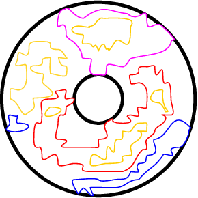 b.
b.
This model is endowed with conformal invariance, so we expect its partition function to be invariant under any conformal mapping. In particular we can study the model on a periodic strip of size ( in the periodic direction), related to the annulus by
| (1) |
The geometry is characterized by the modular parameter
| (2) |
where . As a consequence of conformal invariance, the partition function must depend on the Boltzmann weights of the loops and on the modular parameter only. It is a well-known result that the central charge of the dense loop gas is
| (3) |
where is related to the Boltzmann weight of the bulk loops through
| (4) |
Note that is not restricted to be an integer. Let us also recall the Kac formula
| (5) |
| Contractible | Type | Weight | Parametrization |
|---|---|---|---|
| Yes | Bulk | ||
| Yes | Boundary | , | |
| Yes | Boundary | , | |
| Yes | Both Boundaries | ||
| No | Bulk | ||
| No | Boundary | ||
| No | Boundary |
Now we are ready to present the main result of this article. In full generality, the partition function of the boundary loop model is given by
| (6) | |||||
where the seven parameters appearing are fixed by the seven different loop weights. The relations between all these parameters are given in Table 1. Note that is our notation for .
2 Some algebraic preliminaries
Let us begin by introducing a few algebraic concepts that we will need throughout our discussion. Our model is the densely packed loop model on the tilted square lattice. A very convenient way to think about it is to view it as a face model (see Fig. 2). Each face can be of two different kinds, corresponding to a horizontal or a vertical splitting of the loops.

Each closed loop is given a Boltzmann weight . The loops touching the boundaries are distinguished from the bulk ones in our model, and they are given different Boltzmann weights , or if they touch the first boundary, the second one, or both of them. The total weight of a particular configuration is then where the ’s are the numbers of loops of each kind. We shall later refine these weights to include information about the homotopy class (contractible or not) of each loop.
2.1 The Temperley-Lieb algebra
To begin with, we just drop the distinction of the boundary loops. Then partition function of such a loop model can be reformulated in terms of local operators satisfying some commutation relations that will correctly count the closed loops. The trick is done by the celebrated Temperley-Lieb algebra [20], defined as follows. The Temperley-Lieb algebra defined on strands consists of all the words written with the generators (), subject to the relations
| (7a) | |||||
| (7b) | |||||
| (7c) | |||||
The point of this definition originates in its graphic representation. Represent as an operator acting on strands
then ()–() read respectively
and
Each configuration of loops on a lattice of width can be written as a particular word of the algebra (for example the configuration in Fig. 2, dropping the blobs coming from the boundaries, would be written ). In fact all the configurations can be generated by taking powers of the transfer matrix of the model, which reads
| (8) |
2.2 Boundary conditions and blob operators
In the model we have just introduced, the loops touching the left or right boundaries of the lattice are not different from the other ones. We will refer to this particularly simple case as “free” boundary conditions. In this paper we deal with much more general boundary conditions. They consist in giving a different Boltzmann weight (resp. ) to the loops which have touched at least once the boundary (resp. ). This is encoded in the transfer matrix by the addition of so-called “blob” operators and to the algebra . Their graphical representation consists of a black (resp. white) blob which marks the first (resp. last) strand. acts as
and as
They satisfy the defining relations
| (9a) | |||||
| (9b) | |||||
| (9c) | |||||
and
| (10a) | |||||
| (10b) | |||||
| (10c) | |||||
In what follows, we will assume that is always even. In that case it is possible to have closed loops touching both boundaries. In order to count each of these loops with a weight , we impose the relation
| (11) |
which can be drawn as
The generators , and , subject to the relations (7), (9)–(10) and the quotient (11), thus form the Two-Boundary Temperley-Lieb algebra on strands, denoted . A simpler case to which we shall sometimes refer is the One-Boundary Temperley-Lieb algebra , generated only by the ’s and . The transfer matrix of the two-boundary loop model is then a generalization of Eq. (8)
| (12) |
It generates all the boundary loop configurations on a strip (see Fig. 2) and gives the correct weights to the closed loops in the bulk, and , or to the ones touching the boundaries.
2.3 Generic irreducible representations of 2BTL
Irreducible representations of the Temperley-Lieb algebra are well known, and are closely related to those of the quantum group . When is not a root of unity11 1 Of course here is not the modular parameter defined by (2)., the representation theory of is essentially the same as the one of . In that case, the corresponding irreducible representations of the Temperley-Lieb algebra are said to be generic. The generic representations have a simple graphical interpretation, as the Temperley-Lieb algebra itself. The different modules (representation spaces) are given by configurations of half-loops and strings. For example, consider the Temperley-Lieb algebra on strands , for which there are only three generic modules.
The vertical lines are the strings, and the action of on two strings on the sites , is defined to be zero.
Now if we work with the Two-Boundary Temperley-Lieb algebra (or with ), the generic representation theory is quite similar and has been studied in [12, 11, 16]. The modules consist of the all states formed with half-loops and strings, but the half-loops can be marked with black or white blobs. Note that every black blob is necessarily on the left of every white blob. One can show [11, 16, 19] that the dimension of for is . For example, the module is of dimension for :
This result will play an important role in the sequel, when we will have to deal with Coulomb gas arguments.
Now consider the modules with strings. Half-loops between strings cannot be blobbed, since they are always separated from the boundary by at least one string, so or cannot act on them. The leftmost (resp. rightmost) string can carry a black (resp. white) blob. They can also be orthogonal to the blob, in the sense that they are not eigenstates of the projector , but of the orthogonal projector (“unblob”) . Let us thus mark with a black (resp. white) square the action of (resp. ). Then there is not only one module with strings, but four, depending on the blob status (blobbed or unblobbed) of the leftmost and rightmost strings. For the modules with two strings are
Obviously these modules are related to each other by the blobbed/unblobbed transformations
| (13) |
and this symmetry between the projectors and and their orthogonals and will indeed play some role in our analysis of the loop model.
2.4 Markov trace on 2BTL and the boundary loop model on the annulus
Let us begin by dropping the blobs and the particular boundary weights, and start with the free/free partition function. Then the transfer matrix is given by (8) in terms of the Temperley-Lieb generators ’s. There is an algebraic tool closely linked with the study of the Temperley-Lieb algebra, namely the Markov trace, which is useful for our problem. We give only a naive definition of that tool here. The Markov trace of an element of the Temperley-Lieb algebra is the number which is obtained by identifying the top and the bottom of the diagramatic representation of , upon counting each closed loop with a weight . For example, consider on strands:
Although this object clearly depends on the number of strands , we do not mention it explicitly. Given this naive definition, the Markov trace is associated with the Temperley-Lieb algebra itself, and does not require to know anything about its representations. Note that the Markov trace is not a trace in the common sense: it is not a sum over a basis of states of the diagonal action of . However, there is a well-known relation between the Markov trace and the usual traces over the different generic modules of the Temperley-Lieb algebra. Using , we have
| (14) |
This relation calls for a few remarks. First, we use the convention that is empty if or if . In particular, the sum is finite, and the terms depend on . Then, note that is a polynomial in the variable : , , , etc. They are actually Chebyshev polynomials of the second kind, .
We consider now a modification of the Markov trace, which will be useful for our loop model. We can decide that we draw all the Temperley-Lieb diagrams in instead of and that when we compute the Markov trace, we give a weight only to the contractible loops, and another weight to the non-contractible ones. Again it is convenient to consider an example:
The modified Markov trace has quite the same structure as the previous one. In particular, it can be decomposed on the usual traces over the generic modules exactly in the same way.
| (15) |
This time the coefficient of each trace is a polynomial in , and it is a remarkable fact that it does not depend on at all.
It turns out that we can define the Markov trace (or the modified Markov trace) in the same way for the Two-Boundary Temperley-Lieb algebra , counting the blobbed loops with the appropriate weight , or (or , for non-contractible loops in the case of the modified Markov trace). Recall that contractible loops touching both boundaries appear only if we work with an even number of strands , so the number of strings must always be even, and we write . Again, this object admits a decomposition on the usual traces over the different generic modules
| (16) |
where the are some polynomials in , and (or , , only if we are dealing with the modified Markov trace). The computation of the coefficients can be achieved by various methods, see [11] for a combinatorial proof or [19] for a more algebraic approach. The results are as follows. Let and be such that
| (17) |
and
| (18) |
then
| (19a) | |||||
| (19b) | |||||
| (19c) | |||||
| (19d) | |||||
These equations are related by the blobbed/unblobbed transformation (13). To see this, note that the weight of a non-contractible loop marked with a black square (recall the black square stands for the action of ) is simply . The transformation (13) has thus the effect of changing into , or into . These are indeed the transformations needed to pass from to , or , or .
The physical interest of the Markov trace, or of the modified Markov trace, is that it counts automatically with the correct weight all the loops of a Temperley-Lieb element when the top and the bottom of the diagram are identified. This is exactly what we need to write down the partition function of our loop model. The transfer matrix on strands is an element of the algebra , see (12). We want to work on an annulus of size , so taking periodic boundary conditions in the direction, the partition function of our loop model is just the modified Markov trace of a power of the transfer matrix.
| (20) |
Eq. (16) gives the natural decomposition over the different modules
| (21) |
This relation holds for every and . In particular, it must remain true in the limit with fixed. Then if we introduce the (properly renormalized) characters
| (22) |
the conformal partition function will have the following structure
| (23) |
Hence, the computation of the conformal partition function has been reduced to the determination of the characters .
3 Coulomb gas for the sector without strings
In the previous section we explained why the partition function should have an algebraic structure coming from the Two-Boundary Temperley-Lieb algebra that we have just presented, and hence can be decomposed on different sectors corresponding to the generic irreducible representations of . Hence we are allowed to deal with each sector independently. This section is devoted to the computation by Coulomb gas arguments of the character , defined in the previous section as the trace over the module of . First we detail how to obtain the parametrizations given in Table 1 in the Coulomb gas framework. These parametrizations have also a deeper algebraic origin associated with the Temperley-Lieb algebra [12, 11, 16, 19], but the detailed discussion of this aspect will be deferred to [19].
3.1 A reminder: Coulomb gas on an infinite cylinder
We now want to map our boundary loop model on a height model for which it is simpler to compute some quantities such as correlation functions or partition functions. We recall some classical arguments here. For the loop model on an infinite cylinder, the mapping is well-known. This must correspond to the limit (recall is the periodic direction). First begin by giving each loop an orientation, then interpret the oriented loops as level lines for a height field defined on the cylinder. The height varies by when upon crossing an oriented line. Each loop is counted with a weight , depending on its orientation. The sum over the two orientations then gives the correct initial weight to the original loop. Then it is generally argued that this model renormalizes to a free gaussian model with action
| (24) |
This is however not sufficient to count correctly the loops which wrap around the cylinder. To do this, one has to add two charges at the ends of the cylinder. This modifies the scaling dimension of the vertex operator to
| (25) |
The value of can then be fixed by the following argument. We started from a model in which the height difference when passing through a loop is , so the operator should be marginal. This recquires or , so
| (26) |
The choice of the sign can actually lead to two different phases of the loop model, dense or dilute. We are working with a dense loop model, so we have to choose the solution . To finish, let us determine the central charge of this conformal field theory. The addition of charges at the ends of the cylinder has changed the behaviour of the partition function on the very long cylinder () by a factor . This is sufficient to identify the central charge, since we expect in that limit, instead of without the addition of charges. Then we have
| (27) |
Defining such that , this is nothing but the well-known formula (3).
3.2 Boundaries in the height model
Now we turn to the finite geometry of the annulus, and deal with the boundaries. Begin again by giving an orientation to each loop. The bulk loops are counted with a weight if they are clockwise oriented, and in the other case. The Temperley-Lieb generators ’s hence can be defined as acting on the orientations as shown in Fig. 3. It is not difficult to check that the satisfy the relations (7) also in the oriented loop language.

We must find out how the blob operator acts on the loop orientation. There are four different faces (triangles) with half oriented loops which can be combined to create (see Fig. 4). Two of them conserve the orientation of the loop, which means that there is one arrow coming from the left side of the triangle, and one arrow entering it. The two others do not conserve it: both arrows point in the same direction. It is clear that the two faces which do not conserve the orientation cannot contribute to the weight of a loop touching only this boundary, because the orientation will be conserved everywhere else, so when we close the loop this contribution just vanishes. Now assume that the blob just adds some arbitrary phase factor to a closed loop. Then requiring (), the loop gets a weight instead of . The correct normalization is fixed by (). There remains one free parameter: the phase of the coefficients of the faces which do not conserve the orientation. We end up with the expression of the blob given in Fig. 4, where is our free parameter.

The same can be done for the second blob , so we actually have two free parameters coming from the boundary faces which do not conserve the orientation. Our problem has a global phase invariance, so one of them can be fixed, to give the expression of shown in Fig. 4. All the different loop weights can then be computed in terms of the parameters , and . The weights and are given by the sum over both orientations
| (28) |
and
| (29) |
The weight of a loop touching both boundaries is a sum over four possible configurations of the orientations (see Fig. 5), giving the parametrization
| (30) |
as claimed in the introduction (see Table 1).

3.3 Spectrum in the sector without strings
In the sector without strings, we can compute the conformal character using Coulomb gas arguments. The previous prescription for the operators and gives us a height model with the action (24), with Neumann boundary conditions . Because of the boundary vertices which introduce some magnetic charge in the system, we see that there can be a difference of height if we turn once around the annulus:
Clearly, is the number of boundary vertices which inject charge in the system minus the number of those which take charge from it (see Fig. 4). Such a configuration must be counted with a weight .

In addition, we must treat the non-contractible loops. Note that a non-contractible loop which touch the boundary is no longer a loop in our prescription for the Coulomb gas, because it is broken in several half-loops on the boundary. However, the non-contractible loops which remain in the bulk must be counted correctly (see Fig. 7). Remember that we do not want to compute the full partition function here, but only the character corresponding to the representation of without string . Consider the following instructive example: we want to compute the trace over the module of the following element of
Only states in contribute to this trace
It should be clear why there are exactly states contributing to the trace. The top of the diagram corresponding to our element puts strong constraints on these states. More precisely, it gives all the information about the part which is disconnected from the bottom of the diagram [21]. Then if there are lines (not blobbed, as in our example) going from the bottom to the top of the diagram, the states that contribute to the trace are exactly those we can form with half-loops, wathever their blob status is. In other words, the number of these states is the dimension of the module on strands, that is . A more complete study of this is given in [11]. This conclusion is sufficient for our discussion: each non-contractible loop in the bulk contributes with a weight to the character .
This has an important consequence for our Coulomb gas construction : since each non-contractible loop that we cross when we go from one boundary to another is weighted by , we do not have to put some additional electric charge to correct their weight (unlike the case of the infinite cylinder that we discussed above).

Then, so far, we are able to count correctly the lines going from one boundary to another, and the non-contractible loops in the bulk. The next question is of course: what do we do with the vertices which conserve the charge, which should be given weights proportional to , , etc.? Our guess here is that they do not contribute to the universal part of the character, so does not depend at all on and . The reason for this is that the part involving (resp. ) in (resp. ) is diagonal, so it can be viewed equivalently as a field living on the boundary. We expect any such boundary field to flow towards a fixed boundary condition under RG, which should not depend on (or ). We have checked that conjecture numerically, by transfer-matrix diagonalization and extraction of the finite-size corrections. On the infinite strip of width , the leading exponent is related to finite-size corrections to the free energy per area unit through the well-known relation
| (31) |
We have computed for sizes up to , then extracted the leading exponent using (31) up to order . Although we do not reach a very satisfying precision, our numerical results are compatible with the conjecture that does only depend on (see Fig. 8).
a. b.
b.
Now we are ready to compute the character itself. Let us decompose as
where and . The integration over gives the usual . Then we are left with the contribution of the height difference , counted with a weight as explained above
where . Now we want the expression of some Virasoro character, so we have to work with , not . We perform the Fourier transform using the Poisson formula . The sum becomes
| (32) | |||||
Normalizing the final expression such that the contribution of the identity operator () without its descendents is just , we end up with
| (33) |
Note that, although this character depends only on , it is not true that it does not depend on the loop weights and , because all these parameters are linked by (30). Thus the character is a function of , , and as expected. Note also that, because of the parametrization (30), we expect that is invariant under
| (34) |
and
| (35) |
which is indeed the case for (33), because of the symmetries of Kac’s formula (5).
3.4 Relation with the open XXZ spin chain22 2 This digression can be skipped at the first lecture.
The fact that the representation of is exactly of size and the oriented loop framework we developed above both suggest that there is some link with the celebrated spin XXZ chain, with appropriate boundary conditions. We would like to develop a bit this subject in the following section. In fact, the equivalence between the representation presented above and the so-called spin chain representation of was proved in [16].
It is well-known that the Temperley-Lieb generators can be interpreted as a local Hamiltonian density, that is we can construct a simple Hamiltonian (here with the blob operators)
| (36) |
where and are two (so far unknown) constants.
with
| (37) |
If we parametrize
| (38) |
then our Hamiltonian is, up to an irrelevant additive constant
| (39) | |||||
Note that this is a Hamiltonian for the XXZ chain with non-diagonal boundary terms. This kind of Hamiltonian has been studied in great detail over the recent years [22, 18, 23]. Note also that this Hamiltonian is not hermitian, which was already the case for closed boundaries with an symmetry [24].
Our derivation of the character (33) applies directly to the Hamiltonian (39), so we make the following conjecture about the spectrum of this spin chain. The universal part of the spectrum of does not depend on and when these are positive real numbers. This has been discussed in some detail in [10] in the case of one boundary, and we expect this to be true also in the present case. Then the spectrum should depend neither on the parameters , , nor on and . The only relevant parameter is the difference , which is related to the weights of the loops touching both boundaries in the loop model via (37) and (30). The spectrum of the XXZ Hamiltonian (39) is then given by
| (40) |
where is the "Fermi velocity".
4 The two-boundary partition function
4.1 One-boundary case
In [10], it has been conjectured that the partition function on the annulus with one free boundary condition and one blob is
| (41) |
where we recognize again some polynomials in and . This partition function hence has the structure we have detailed in the previous section, but on the One-Boundary Temperley-Lieb algebra . So far, we have failed to provide some Coulomb gas arguments to derive the exponents . Strong numerical evidence has been given in [10] for general , and exact results have been obtained from Bethe ansatz when is an integer [17]. Many of these results have been rederived since by Kostov using 2d quantum gravity techniques [14, 15]. Note the consistency with our computation of from the previous section : the leading exponent we expect from (33) is . The one-boundary case should be recovered from and , that is and . We see that is indeed the leading exponent appearing in (41). A more precise analysis of the relation between the character for two boundaries and the character in (41) also exists, although it recquires more representation theory for the algebra . We will report on this in [19].
4.2 Boundary states and the partition function
Now we turn to the computation which is the core of this paper, and we determine completely the partition function of our two-boundary loop model in the most general case. The main idea of this computation follows the work of Cardy on minimal theories [25]. We start from the one-boundary partition function , and compute its modular transform. The result is then interpreted as a scalar product between an initial boundary state and the final state , with an evolution operator inserted (see Fig. 9). Then we argue that this result together with the knowledge of the sector without strings is sufficient to guess the partition function of the form . We conclude by computing the modular transform back, and get the general partition function in the form (23).
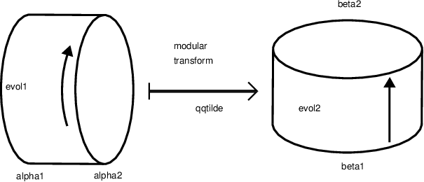
Modular transform of the one-boundary partition function:
What with loops touching both boundaries?
Something special must happen in the sector without strings, because of the loops touching both boundaries. The one-boundary partition function may be seen as a very special case of the two-boundary one, when and . Thus, in the one-boundary partition function, the character given by (33) is present, with the special value . However, for a generic value of , the exponents have no such special value. On the other hand, we expect all the exponents in the string sectors to be completely independent of , since they cannot depend on the weight of loops touching both boundaries. Hence, in this respect, the sector without strings decouples from all the other sectors. In particular, the formalism shown in Fig. 9 should apply if we simply cancel the contribution coming from the sector without strings. At the end of the computation, because of the form of the partition function (23), it will be sufficient to add with giving the correct weight to the loops touching both boundaries, see (30). We have then
| (43) | |||||
Boundary states:
Recall that the free boundary condition on the boundary actually corresponds to . What we want to do now is to identify the terms of
| (44) |
where the sum runs over all the primary exponents appearing in (43), and the states satisfy . We have to distinguish the two sets of exponents appearing in (43).
- •
- •
: This time Eq. (43) seems to give simply
a result which is independent of . This actually would lead to absurd conclusions. Indeed, we work in the string sectors, which all give non-contractible loops, so we expect all the terms to be affected somehow by the weights , and . The only terms which are completely independent of these weights appear in the sector without string, and we have cancelled this contribution. This contradiction comes from the fact that is even in , so when we take the sum over all the exponents, only the even part of remains. Inspired by the form of the coefficients we have already encountered, we can try the simple but non-trivial inclusion of the following odd term in
leading to the generalization
(46)
Modular transform:
Although the (partly guessed) relations (45) and (46) seem quite complicated, they lead to quite a nice formula when we go back to the “open string channel” (see Fig. 9). To see this, we need once again to perform a modular transform. The two sums appearing in (44) are now
| (47) |
and
| (48) | |||||
We can compute the modular transform of each part independently, and add the contributions in the end. Let us begin with . The product can be decomposed as
is then of the form
and is a sum over . Let us write and . We use the Poisson formula to compute the modular transform of . Note that we also use as usual. The sum appearing in the computation is
Putting all things together, we get
| (49) |
Now consider the case of . The computation is quite similar. First we have to decompose the sinus product. Let , then
Then we use Poisson’s formula to get in the end
and after some relabelling of the indices, we have
| (50) | |||||
The two-boundary partition function:
Adding the terms (49) and (50), we find that the total contribution of all the string sectors is
| (51) |
If we now take into account the sector without strings and add its conformal character , we obtain the partition function (6) of our loop model, as claimed in the introduction of this paper. This partition function has the form (23) as expected. We are now able to identify all the conformal characters corresponding to the different sectors.
| (52a) | |||||
| (52b) | |||||
| (52c) | |||||
| (52d) | |||||
Note that these characters are all related by the blobbed/unblobbed transformation (13).
5 Comparison with known results
5.1 Critical percolation on the annulus
As a first simple application of our result, we can turn to the critical percolation problem on an annulus. Critical percolation corresponds to , and in that case the partition function (6) is simply
| (53) |
To see this, it is sufficient to note that our partition function reduces to the one-boundary partition function (41) when and . The one-boundary case itself reduces to the free/free case when . Then for , it is easy to see that using Euler’s pentagonal identity. Now if we want to compute, for example, the probability that there is at least one contractible percolation cluster going from one boundary to the other, we have to vary the weight of loops touching both boundaries . Indeed, each percolation cluster is encircled by exactly one loop, and each cluster touches a boundary if and only if its surrounding loop touches it. Since we know that does only appear through in the conformal character , we have
| (54) |
and then
| (55) | |||||
which agrees with [26].
5.2 Relation with -state Potts models
It is a well-known result that the -state Potts model can be reformulated as a dense loop gas with the loop fugacity . Let us recall here how this can be achieved. The Potts model can be defined on the square lattice, with a spin living on each site. Only the neighbouring sites interact, and the partition function is the sum over all the Potts spin configurations
| (56) |
and this is rewritten as
| (57) |
with . Then the most important step is to interpret (57) as a random-cluster (Fortuin-Kasteleyn) partition function. For a given Potts configuration, the FK clusters live inside the Potts clusters.
| (58) |
Taking the trace over the Potts configurations gives the Potts partition function in its Fortuin-Kasteleyn representation
| (59) |
In the FK representation, the mapping to the loop model is obvious: one has to draw all the loops which encircle the FK clusters or the clusters on the dual lattice (see Fig. 10). Now let be the number of loops, the number of clusters and the number of dual clusters. Clearly, . Moreover, Euler’s formula gives . Then, up to an unimportant global factor, (59) becomes
| (60) |
It is well-known that the Potts model is critical when it is satisfies the self-duality relation . In that case, (60) is exactly the partition function of a loop gas with fugacity .

It is not difficult to generalize the previous discussion to the boundary case. Let us assume that the Potts spins living on the boundaries are restricted to some subsets and . Let
| (61) |
then taking again the trace over Potts configurations we get the following relation instead of (59)
| (62) |
where is the number of bulk clusters, and , , are the number of FK clusters touching the boundary , , or both of them. Introducing the number of loops of the same type , , , it is clear that , and since each boundary cluster is encircled by exactly one boundary loop. For the bulk loops, this is different because each one can encircle either a FK cluster or a dual cluster, so we still have . Now Euler’s relation gives . Up to a global factor, (62) becomes
| (63) |
Again, we can impose the self-duality relation and then the identification of the loop weights is straightforward:
| (64) |
At this point we have given the correct weight to all contractible loops. In this article we are interested in a loop model on an annulus, so we have to take care about the non-contractible loops. This turns out to be non-trivial, and rather crucial if we want to recover some known partition functions of the Potts model on the annulus. The subtlety comes from the non-contractible FK clusters which touch both boundaries, which must be restricted to the set . However, in the loop model these configurations are those with exactly two non-contractible loop, each one touching one boundary. Such configurations are counted with a weight . To solve this problem, we must identify the term coming with the coefficient in the loop partition function (6), and give it the correct weight to get the Potts partition function.
Let be this term in the loop partition function. To identify this term, it is necessary to analyse carefully the polynomials (19). These can actually be written in terms of the Chebyshev polynomials of the second kind , as [11]
| (65) |
with similar expressions for the other polynomials , obtained by using the blobbed/unblobbed transformation (13), which maps on and/or on . With those relations the identification of is straightforward, noting that the constant coefficient of the polynomial is .
| (66) |
Thus we have found the precise relation between our loop partition function and the Potts one
| (67) |
where all the loop weights are given by (64) for the contractible loops, and , , for non-contractible ones. Of course we could have improved slightly the mapping by distinguishing Potts clusters according to homotopy. However, this will not be necessary to recover the known results about the Potts model.
5.2.1 Ising model
We would like to use (67) to recover some results about the Ising model on an annulus, which appeared in [25, 9]. Assume for example that the Ising spins are fixed to on the first boundary and to on the second one. This corresponds in our formalism to , and . Then all the parameters (see Table 1 for the parametrizations) of the loop model are fixed: we have , , . Eq. (6) then gives
| (68) | |||||
and adding the term (66) as in (67), we get the Ising partition function
| (69) | |||||
Consider the second term between the brackets, which comes with a factor . Consider this term twice, and once make the reindexation , , and the second time , . The first term thus obtained cancels almost all the terms in the first sum between brackets, and the second one almost all those of the third sum. Collecting what remains after these cancellations, we have
| (70) | |||||
Now we write and then
| (71) | |||||
Recall the Kac formula (5) to see that , so all the terms combine to form the sums
| (72) |
Again use the Kac formula and (recalling that ) to see that and then
| (73) |
Here we recognize the Rocha-Caridi formula, and we conclude that
| (74) |
as expected from [25]. We could have done the same calculation for the spins fixed to on both boundaries. The computation is exactly as the previous one, except that so this time. This would have led to
| (75) |
which is again a result of Cardy [25]. The other boundary conditions, such as for example, reduce to a computation with the one-boundary partition function, which has been studied in [10]. Again all the results agree with those of [25].
5.2.2 Three-states Potts model
When the Potts spins have three colours A,B,C. For example, we can compute the partition function with all spins fixed to A or B with equal probability on the first boundary, and to B or C on the second one. We have then , , so the parameters (see Table 1) of the loop model are , , . The computation is exactly as in the Ising case. Eq. (67) gives
| (76) | |||||
Once again we see that the double sums actually collapse to give
| (77) | |||||
Using the Rocha-Caridi formula, we finally obtain
| (78) |
which agrees with [25]. All the results from this reference concerning the Potts model can be deduced from our loop partition function (6), with the relation (67).
6 Refined crossing formulae for percolation on the annulus
It should be obvious that the seven-parameter partition function (6) harbours many more geometrical applications than the known ones presented in the preceding section. As an illustration we present here just one simple example.
Consider the continuum limit of critical percolation on an annulus of aspect ratio , and recall that . Let be the probability that no cluster wraps the periodic direction, and let be the probability that there are precisely wrapping clusters which are moreover constrained by the values of the indices . When (resp. ) the leftmost cluster is constrained to touching (resp. to not touching) the left rim; similarly constrains the behaviour of the rightmost cluster.
Since we have obviously
| (79) |
and since by symmetry, this suffices determine all . Note also that by an easy duality argument we have for .
We find the following explicit results for , here given to order :
| (80) |
and . The evaluation of the complete series for aspect ratio leads to the following numerical values:
| 0 | 0.6364540018880 | |||
|---|---|---|---|---|
| 1 | 0.3615910259567 | 0.2770671481561 | 0.0413139498152 | 0.0018959781702 |
| 2 | 0.0019548143402 | 0.0018959781702 | 0.0000293394720 | 0.0000001572261 |
| 3 | 0.0000001578149 | 0.0000001572261 | 0.0000000002943 | 0.0000000000002 |
These values could presumably be verified by numerical simulations in a square geometry.
7 Conclusion
In this article we have studied a densely packed loop model on the annulus, with general loop weights that distinguish the two boundaries and the homotopy class of the loops. The main result is the exact seven-parameter continuum limit partition function (6). We have verified that a range of special cases of this expression agree with existing results in the literature, and used it to derive new refined crossing probabilities in critical percolation.
The directions for future work are quite numerous [19]. Let us discuss briefly a few of them:
- •
Distinguishing both rims of the annulus by non-trivial boundary conditions is related with properties of boundary condition changing operators. Resulting fusion rules are encoded in the result (6). An intriguing—and to our knowledge novel—feature is that the fusion here depends on a parameter which is unrelated to those characterizing the two individual operators.
- •
Specializing the two-boundary model to simpler cases gives rise to a rich hierarchy of restrictions. For instance, the two-boundary model with and becomes the one-boundary model, and with this in turn becomes the standard (“zero-boundary”) Temperley-Lieb model. Moreover, in each case there are “magical” values of the weights, typically corresponding to one of the -type parameters taking an integer value. Each of these restrictions corresponds to the disappearence of some of the states in the transfer matrix, the vanishing of certain eigenvalue amplitudes, and the reorganization of the Hilbert space into new modules. There is a rich algebraic meaning of this truncation hierarchy.
- •
The present work pertains to the dense phase of the O() model. In the dilute case the possibilities are richer: in addition to the boundary-specific -type weights, one can weigh differently the boundary monomers depending on the type of loop to which they belong. This gives rise to several surface transitions. Some of those will be insensitive to the values of the -type parameters, others will correspond to the usual swapping of indices (i.e., in the Kac formula), and yet others lead to genuinely new behaviour.
Acknowledgements
We thank J. Cardy, I. Kostov, R. Nepomechie and B. Nienhuis for helpful comments and for correspondence. This work was supported by the European Community Network ENRAGE (grant MRTN-CT-2004-005616), by the Agence Nationale de la Recherche (grant ANR-06-BLAN-0124-03), and by the ESF Network INSTANS.
References
- [1] I. Affleck, Lectures given at the 2008 Les Houches summer school Exact methods in low-dimensional statistical physics and quantum computing, cond-mat/08093474.
- [2] V. Schomerus, Lectures on branes in curved backgrounds, hep-th/0209241.
- [3] I. Gruzberg, A.W.W. Ludwig & N. Read, Phys. Rev. Lett. 82, 4524, 1999.
- [4] J. Cardy, Phys. Rev. Lett. 84 (2000) 3507
- [5] P.A. Pearce, J. Rasmussen & J.-B. Zuber, J. Stat. Mech. 0611, P017, 2006.
- [6] N. Read & H. Saleur, Nucl. Phys. B 777, 316, 2007; Nucl. Phys. B 777, 263, 2007.
- [7] B.L. Feigin., A.M. Gaiutdinov, A.M. Semikhatov and I.Yu. Tipunin, Nucl. Phys. B 757, 303, 2006.
- [8] J. Cardy, Lectures given at the 2008 Les Houches summer school, Exact methods in low-dimensional statistical physics and quantum computing, hep-th/08073472.
- [9] H. Saleur & M. Bauer, Nucl. Phys. B 320, 591, 1989.
- [10] J.L. Jacobsen & H. Saleur, Nucl. Phys. B 788, 137, 2008.
- [11] J.L. Jacobsen & H. Saleur, J. Stat. Mech. P01021, 2008.
- [12] P. Martin & H. Saleur, Lett. Math. Phys 30, 189, 1994.
- [13] P.P. Martin and H. Saleur, Comm. Math. Phys. 158 (1993) 155.
- [14] I. Kostov, J. Stat. Mech. 0802, P003, 2007.
- [15] J.-E. Bourgine & K. Hosomichi, arXiv:hep-th/08113252.
- [16] J. de Gier & A. Nichols, arXiv:math/0703338.
- [17] A. Nichols, V. Rittenberg & J. de Gier, J. Stat. Mech. 0503, P003, 2005; A. Nichols, J. Stat. Mech. 0601, P003, 2006; A. Nichols, J. Stat. Mech. 0602, L004, 2006.
- [18] R.I. Nepomechie, Jour. Phys. A 37, 433, 2004; R.I. Nepomechie & F. Ravanini, Jour. Phys. A 36, 11391, 2003.
- [19] J. Dubail, J.L. Jacobsen & H. Saleur, in preparation.
- [20] H.N.V. Temperley & E.H. Lieb, Proc. Roy. Soc. London A 322, 251, 1971.
- [21] J.-F. Richard & J.L. Jacobsen, Nucl. Phys. B 750, 250, 2006.
- [22] J. de Gier & P. Pyatov, J. Stat. Mech. 0403, P002, 2004.
- [23] C. Ahn & R.I. Nepomechie, Nucl. Phys; B 676, 637, 2004.
- [24] V. Pasquier & H. Saleur, Nucl. Phys. B 330, 523, 1990.
- [25] J. Cardy, Nucl. Phys. B 324, 581, 1989.
- [26] J. Cardy, J. Phys. A 35, L565, 2002.