Skyrmion in spinor condensates and its stability in trap potentials
Abstract
A necessary condition for the existence of a skyrmion in two-component Bose-Einstein condensates with symmetry was recently provided by two of the authors [Phys. Rev. Lett. 97, 080403 (2006)], by mapping the problem to a classical particle in a potential subject to time-dependent dissipation. Here we further elaborate this approach. For two classes of models, we demonstrate the existence of the critical dissipation strength above which the skyrmion solution does not exist. Furthermore, we discuss the local stability of the skyrmion solution by considering the second-order variation. A sufficient condition for the local stability is given in terms of the ground-state energy of a one-dimensional quantum-mechanical Hamiltonian. This condition requires a minimum number of bosons, for a certain class of the trap potential. In the optimal case, the minimum number of bosons can be as small .
I Introduction
Topological defects often play a fundamental role in our understanding of phases of matter and the transitions between them. The best understood examples are probably vortices and vortex-loops in superfluids and magnets in two and three dimensions, which are responsible for the very existence of the high-temperature phase, and completely determine the universality class of the phase transition [1]. The next in order of complexity are the topological defects in the -symmetric Heisenberg model, which allows skyrmions in two dimensions [2] and hedgehogs-like configurations (a point defect around which spins point outward) in three dimensions [3]. While the former only renormalize the coupling constant, the role of the latter is less clear [4]. All of the above, however, represent configurations topologically distinct from vacuum, which provides them with local stability.
In this paper, we study the stability of the topologically non-trivial skyrmion configuration in theories with symmetry. Such a symmetry arises in complex condensates with an internal spin--like quantum number [5], for example. Realizations of such spinor condensates are found in models of inflatory cosmology [6], Bose-Einstein condensation of 87Rb [7], and bosonic ferromagnetism [5, 8], and in effective theories of high-temperature superconductivity [9, 10] and of deconfined criticality [11]. The Higgs sector of the Weinberg-Salam model of electroweak interactions represents another closely related example, with a spinor condensate coupled to gauge fields. In our problem in three dimensions, there exists a topologically non-trivial mapping to the order-parameter space, thanks to the fact that the third homotopy group of is the group of integers. However, the topology alone turns out to be insufficient to guarantee local stability of the skyrmion. This may be understood already in terms of the classic Derick theorem [12]. Recently, a more general proof that the skyrmion cannot be a stationary point of the action for the spinor Bose-Einstein condensate (BEC) in free space was given by two of the present authors [13], based on the analogy between the Euler-Lagrange equations and the classical mechanics of a particle in a time-dependent dissipative environment [14]. The advantage of this alternative point of view at the old problem is that it provides one with a simple way of constructing the external potentials which would indeed lead to skyrmion as the solution of the Euler-Lagrange equations. In Ref. [13], three such special potentials were presented. In this paper, we further develop this approach.
First we analyze the construction of the solution based on the ansatz proposed in Ref. [13]. There, a time-dependent dissipation which is odd in time was introduced, to allow an odd solution. However, we find that the symmetry argument does not always work, and there is a critical dissipation strength above which the odd solution no longer exists even for an odd dissipation. Next, we study the stability of the skyrmion in a generalized class of the potentials introduced in [13] with respect to small variations. We map the problem to an effective quantum-mechanical eigenvalue problem and determine the region of local stability in the parameter space. A particularly interesting result of our analysis is that the stable skyrmion requires a minimal number of particles in the trap, estimated here to be in the optimal case.
The paper is organized as follows. In Sec. II, we present basic formulation of the problem. A classical equation of motion with time-dependent dissipation determines the skyrmion solution. On the other hand, a quantum mechanical eigenvalue problem determines the local stability of the solution. In Sec. III, we discuss the construction of the skyrmion solution based on the odd-function ansatz. We determine the critical dissipation strength, which separates the region with and without a skyrmion solution. In Sec. IV, we present the numerical solution of the equation of motion for a few cases. The existence of the critical dissipation strength, as well as related theoretical predictions, is confirmed numerically. Furthermore, the local stability of the obtained solution is also analyzed by solving the quantum-mechanical eigenvalue problem. The minimal number of bosons required to satisfy the sufficient condition for the local stability is numerically obtained as a function of parameter. Section V is devoted to summary of the paper.
II General discussion on the skyrmion solution
II.1 Basic equations
We begin by reviewing the derivation of the skyrmion solution for the two-component (spinor) BEC in an external potential, formulated previously in Ref. [13]. The derivation is based on the Euler-Lagrange equations, and leads to the necessary condition for the existence of the skyrmion solution. We will then proceed to examine the stability of the skyrmion by taking into account the second-order variation.
Let us consider the two-component bosons in three-dimensional continuum space in the external confinement potential . The system can be described by the following effective action via the path integral formalism [1]:
| (1) |
where is a two-component bosonic field with the mass , which satisfies the periodic boundary condition , where . The bosons interact with each other by the repulsive contact interaction . is the chemical potential. In addition to the usual symmetry corresponding to the conservation of the number of the bosons, the system is invariant with respect to the global transformation of the boson field , where is an matrix. As usual, the trap potential has been included in the definition of the action or the corresponding Hamiltonian.
Next, we introduce the dimensionless parameters and fields by rescaling:
| (2) | ||||
| (3) | ||||
| (4) |
where is the constant length scale. Effective action (1) may be written now in terms of the dimensionless parameters as
| (5) |
Let us focus on classical field configurations independent of the imaginary time. It will prove convenient to represent the -independent field by an amplitude and a two-component complex spinor configuration : . The spinor is normalized as . In terms of and , we can rewrite the effective action for the -independent field configuration ,
| (6) |
where we have used the relation deduced from the normalization condition for the spinor . The stationary state also needs to satisfy the boundary condition
| (7) |
It guarantees the stability of the solution with respect to small rotations of the spinor at the infinitely remote boundary of the system.
Let us take the variation in action (6) around the classical field using the following expressions for the amplitude and the spinor configuration:
| (8a) | ||||
| (8b) | ||||
where and are the variations around for the density profile and the spinor configuration, respectively. and are the amplitude and the spinor of some stationary field configuration. In particular, will assume a form corresponding to the skyrmion solution, which is to be defined shortly. Substituting into the action, action (6) can be written as
| (9) |
where is the Lagrangian density related to the th order of the variation and . The Lagrangian densities up to the second-order variation are then expressed as
| (10a) | ||||
| (10b) | ||||
| (10c) | ||||
II.2 Mapping to a problem in classical mechanics
Setting for any and leads to the Euler-Lagrange equations giving the extremum of the action:
| (11) | ||||
| (12) |
The latter equation follows by recalling that , so that .
For simplicity, we further assume that the external potential is spherically symmetric, , where . Then, in terms of the spinor configuration, we can adopt the most general ansatz with the same spherical symmetry [3],
| (13) | ||||
| (14) |
where . At the infinitely remote boundary, we impose , where is any integer. If we additionally adopt the boundary condition , and changes from to as changes from to infinity, ansatz (14) means that the spinor configurations wraps the three-dimensional sphere times, and thus corresponds to the skyrmion solution. Hereafter, we restrict the discussion to the simplest case of .
Let us then consider Euler-Lagrange equations (11) and (12) for skyrmion (13) and (14). Substituting Eqs. (13) and (14) into Euler-Lagrange equations (11) and (12), we obtain the following differential equations:
| (15) | ||||
| (16) |
To analyze these differential equations, it is very convenient to change the variable from to . Then, as , . Rewriting Eq. (16) in terms of , we obtain
| (17) |
where . This equation can be regarded as describing classical motion of a particle in an external potential with dissipation. and , respectively, correspond to the potential energy and the “time”-dependent dissipation, given by
| (18) | ||||
| (19) |
where . In terms of skyrmion solution, boundary conditions for may be written as at the origin of the three-dimensional space, and , at the infinitely remote boundary. These boundary conditions in terms of translate into
| (20) |
Integrating equation of motion (17) with respect to , and imposing the set of boundary conditions (20), one obtains the following necessary condition for the existence of the skyrmion solution:
| (21) |
The condition implies that the total integrated dissipation in the problem vanishes [15]. It is now clear that a skyrmion solution exists only when the density profile takes a special form, so that the solution satisfies condition (21).
II.3 Stability of the skyrmion and a quantum-mechanical eigenvalue problem
The integral condition provides only the necessary condition for the existence of the skyrmion solution, but does not guarantee its stability. Here, we analyze the second-order variation, to obtain a further condition for the stable skyrmion solutions.
Let us assume that an appropriate external potential is given so that the Euler-Lagrange equations allow a skyrmion solution and . For the obtained skyrmion solution to be stable against local variations, the second-order variation in Lagrangian (10c) has to be positive. Obviously, the second term in Eq. (10c) is always positive. The positivity of the first term in Eq. (10c) for arbitrary and is thus a sufficient condition for the local stability of the skyrmion. The first term being a quadratic form of , its positivity for an arbitrary is equivalent to positive definiteness of the linear operator
| (22) |
where
| (23) |
Positive definiteness of means that all the eigenvalues of are positive. In fact, may be interpreted as the quantum-mechanical Hamiltonian for a single particle in the external potential . The (sufficient) condition for the stability then corresponds to the ground-state energy of the Hamiltonian being positive.
The external potential depends on both the spinor part and the density profile of the skyrmion, as set by the Euler-Lagrange equations. According to Eq. (11), is also spherically symmetric.
We should mention that even if the ground-state energy of Hamiltonian (22) is negative, it is possible that second-order variation (10c) is still positive, if the positive second term is large enough. We, however, will be unable to say more about this issue, and our discussion will be limited to the sufficient condition for the skyrmion stability formulated above.
III Construction of skyrmion solutions for trapped BECs
III.1 Odd-function ansatz
Let us discuss a few concrete examples of skyrmion solutions. In a usual formulation, we seek a solution for a given trap potential . However, as discussed in Ref. [13], a generic trap potential does not allow a skyrmion solution. Thus, we solve the problem backward: first we determine the dissipation so that equation of motion (17) has a solution which represents a skyrmion. The assumed dissipation determines the density profile of bosons. Finally, the trap potential is determined so that it reproduces the chosen .
For convenience, here we introduce the new variable
| (24) |
Equation of motion (17) is then rewritten as
| (25) |
Boundary conditions (20) read, in terms of ,
| (26) | ||||
| (27) |
We observe that the boundary conditions at would be automatically met if obeys boundary conditions (26) at and is an odd function:
| (28) |
This is sufficient to satisfy the original conditions (26) and (27), but not necessary. However, here we focus on finding the solutions which are odd in , because it is easier than solving the general problem.
Equation (25) is invariant under
| (29) |
if is also odd in . Thus we choose an odd so that we can find an odd solution . Although this is a somewhat restrictive choice, it is a useful ansatz in construction of skyrmion solutions.
However, it turns out that some choice of odd actually does not allow an odd solution which satisfies the boundary conditions at . Roughly speaking, if the dissipation is too strong, the particle which starts at with a vanishing speed at can not reach at . We will examine two forms of odd as examples:
| (30) | ||||
| (31) |
where is a positive parameter. As we will demonstrate, for each case there is a critical parameter ; an appropriate odd solution exists only if .
The existence of an odd solution can be discussed in the following manner. First we impose boundary conditions (26) only at . Of course, they do not completely fix a solution but allow a family of different solutions. This is evident by recalling that the trivial solution satisfies Eq. (26).
Then we attempt to find, among the solutions, the one which satisfies . This would be the desired odd solution. The particle falls off the hill and approaches the potential minimum . If the particle is still rolling down the hill () when , the particle is only accelerated by the negative friction for and it must eventually reach at some positive . Namely, for any dissipation strength, there is a solution which satisfies at a positive . On the other hand, while , the velocity should always be positive. Thus the smallest solution of changes continuously. Therefore, if there is another solution which satisfies at a negative , there must be an odd solution with thanks to the intermediate value theorem.
III.2 Constant- regime
In either case of Eq. (30) or (31), we observe that, for ,
| (32) |
This simply represents the constant-dissipation coefficient. The equation of motion
| (33) |
in this regime is independent of time. Thus, for any solution , the translated solution is also a solution for any . Let us discuss the solutions of this equation. This will turn out to be useful in determining the critical parameter for the original equation of motion (25).
As we will see later, when , the particle comes very close to the minimum () while still in the constant- regime (). For small , we may use the linearized equation of motion
| (34) |
instead of the full nonlinear equation (33). Its solution can be easily obtained as
| (35) |
where
| (36) | ||||
| (37) |
One can choose an arbitrary large positive , thanks to the translation invariance in time. On the other hand, taking a large negative (for a fixed ) makes large, and may invalidate linear approximation (34).
When , are a complex conjugate pair and the solution represents a damped harmonic oscillation. In this case, there is obviously a solution which reaches within Eq. (33). Namely, there is a solution which satisfies at a negative . As we discussed in Sec. III.1, the intermediate value theorem assures that there is an odd solution with in this case. This means that .
Thus, in the following, we focus on . Then, the first term is the leading one in the . The second term vanishes more quickly, but the subleading contribution determines the critical exponent as we will show later.
In fact, in discussing the subleading contribution, we must also consider the nonlinear effects which were ignored in Eq. (34). We introduce the scaling of by the replacement . We are interested in the limit in which the original is small, namely . The equation of motion now reads
| (38) |
Considering the limit and retaining only the leading nonlinear term, we obtain
| (39) |
We consider a series expansion of the solution in terms of , which can be regarded as a perturbative expansion of nonlinear effects.
The lowest order is given by the solution of linearized equation (34). The next order is of , and is given by a solution of
| (40) |
This is an inhomogeneous linear differential equation on for a given , which can be solved by a standard method. Taking the as general solution (35) of the linear equation, we find the special solution
| (41) |
where only the leading term is given. The general solution also contains solutions of the corresponding homogeneous equation. However, they have the same form as and can be ignored in the following.
Combining with the solution of the linearized version [Eq. (35)], the leading and next-leading terms in the limit can be written as
| (42) |
where
| (43) |
Namely, when , the next-leading term comes from the nonlinear effect instead of the term proportional to .
Recalling that the particle approaches from , . The constant is determined by the solution of nonlinear equation of motion (33) with the constant dissipation and boundary conditions (26). The solution gives the effective initial conditions for the linearized equation.
Numerically solving Eq. (33) with Eq. (26), we find that, the ratio increases monotonically, as shown in Fig. 1, when . This observation implies that in linear regime (42).

In fact, when the nonlinear effect gives the next-leading term, it follows from Eq. (41) that
| (44) |
When the subleading contribution within the linear equation gives the next-leading term, we do not have a proof but seems certain from numerical results.
III.3 Critical parameters in the step-function case
Let us consider the step-function case of Eq. (30). Here, the solution of Eq. (33) discussed in Sec. III.2 gives the “initial condition” at for the equation without the dissipation. If the particle is very close to the minimum () at , the successive motion is just a harmonic oscillation with the angular frequency of . We will show later that for , indeed holds at .
The phase of the oscillation is given as
| (45) |
When , the particle just manages to reach at . For that, we need to give the optimal initial condition at , namely, with the maximum possible value. As discussed in Sec. III.2, for Eq. (33) monotonically increases. Thus the optimal initial condition [maximum possible ] is realized by letting the particle spend infinite time around before , namely, by taking . In this limit, the first term in Eq. (42) dominates and the initial condition at is given by
| (46) |
We emphasize that depends only on the ratio between the “initial” velocity and “initial” coordinate on , which converges to a finite value in the limit . The time required to reach the minimum () in the harmonic oscillation is
| (47) |
The critical dissipation coefficient in this problem is thus given by
| (48) |
so that the particle arrives at at . Therefore we find
| (49) |
In the limit , , and thus both and vanish. This implies that the velocity of the particle when it reaches the potential minimum, , also vanishes. Let us discuss its critical behavior, namely, how depends on when .
For , if we take the particle reaches the minimum before because . By letting the particle spend less time around by taking a smaller , we can change the initial condition at so that is smaller than the optimal value (46). Therefore, for , there is a solution which reaches the minimum at . Combining
| (50) |
with Eq. (42), for small we find
| (51) |
This implies that
| (52) |
As a consequence,
| (53) |
which leads to
| (54) |
In the present case, for , , namely, . Thus we obtain
| (55) |
For , even under the optimal condition , the particle cannot reach at . In this case, the odd solution does not exist.
III.4 Critical parameters in the tanh case
Now let us consider case (31). The mathematics is somewhat more complicated but the physics is quite similar to the previous one.
As in the previous problem, for , we can assume that the particle comes very close to the minimum at negative time. The linearized equation of motion, with the full time dependence of the dissipation, reads
| (56) |
This equation has the general solution
| (57) |
where are constants, and and are associated Legendre functions.
Let us first discuss the asymptotic behavior of the above solution in the limit . In this limit, equation of motion (56) reduces to Eq. (34), and thus the solution should be equivalent to Eq. (35). In fact, using
| (58) |
and the asymptotic expansion of the associated Legendre functions, we have confirmed that Eq. (57) coincides with Eq. (35) in the limit .
Now, the similar discussion as in Sec. III.3 applies here. Namely, the numerical solution implies that increases monotonically. Thus, the optimal condition for reaching is realized when the particle spends infinite time around before . This can be done by replacing with and taking . In this limit, the asymptotic behavior of the solution in the regime is dominated by .
In the following, we demonstrate that
| (59) |
To show that, let us set . The two independent solutions reduce to
| (60) | ||||
| (61) |
in the limit . This implies that, under the optimal condition, the solution consists only of the term.
On the other hand, for , the Taylor expansion around reads
| (62) | ||||
| (63) |
Namely, the solution consisting only of the term just crosses on . By perturbing the solutions around , it can be shown that the solution with exists for . This means that is indeed the critical value .
III.5 Requirement of a finite number of bosons
We consider the situation where all the bosons are confined in the finite space by external trap potential . If it is to be realized in experiments, the total number of the bosons should be finite. This gives an additional requirement independent of the stability.
In terms of the density profile , the condition of the finite number of bosons is easily given as
| (65) |
For the choice of the dissipation [Eq. (31)], the density profile can be obtained via Eq. (19) as
| (66) |
where is a positive constant which appears from the integration of Eq. (19). The density profile in the case was discussed in Ref. [13]. in the integral of Eq. (65) asymptotically behaves as for large . Accordingly, for the total number of the trapped bosons diverges, violating condition (65). Hereafter, we focus on the finite-bosons case, .
IV Numerical solution for a skyrmion
IV.1 Solution of the equation of motion
Equation of motion (17) determines for a given choice of . While we have determined critical parameters in Sec.III, unfortunately, the full solution cannot be obtained analytically. Thus, here we solve Eq. (17) numerically. The numerical solution can be also used to check the analytical predictions on the critical parameters discussed in Sec. III.
To reiterate, we seek a solution which satisfies the boundary conditions at [Eq. (20)]. For an odd , which is the case we discuss in this paper, such a solution satisfies Eq. (28). To find the odd solution for an odd , it is enough to require
| (67) |
together with either of the boundary conditions at or in Eq. (20).
Based on this observation, we adopt the so-called “shooting method” in the numerical scheme, which is explained in Appendix A. In Fig. 2, we show the numerical result for the case of Eq. (31).

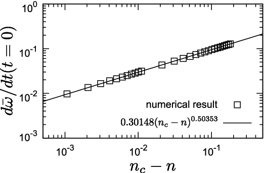
Here, we observe that the velocity at vanishes as the dissipation parameter approaches . This is indeed consistent with the analytic prediction on the critical parameter and on the critical behavior. To see this more clearly, in Fig. 3, we show the numerical result on as a function of . The result is in good agreement with the analytic predictions. We also have made a similar comparison for step-function dissipation (30) in Fig. 4, and found agreement with analytic predictions (49) and (55) as well.

IV.2 Stability of the skyrmion and minimal number of bosons
We have shown that the skyrmion as a solution of the Euler-Lagrange equation exists for , and obtained the solution numerically. The spinor configuration is given by the solution of a classical mechanics problem. The density profile can then be obtained.
The next step is to examine the stability of the obtained skyrmion. Note that there is a free parameter appearing in density profile (66). Substituting the obtained and into Euler-Lagrange equation (16), the trap potential realizing the skyrmion is obtained. Then, we find that depends on and as a function of . This information on , , and determines the effective potential (23), shown in Fig. 5.


In order to obtain the stable skyrmion, larger than the critical value is needed. Indeed, calculating the ground-state energy of quantum-mechanical Hamiltonian (22) by use of the numerical diagonalization method, it is found that as increases, the critical value diverges as approaches , as shown in Fig.6.

Finally, let us investigate the total number of the trapped bosons for some values of and . Due to Eq. (66) for the density profile, the number of bosons monotonically increases as a function of : it is proportional to . For a given , the number of the trapped bosons is minimal at . The dependence of the number of the bosons in is then shown in Fig. 7. We find the minimum at , with the value of . It is comparable to the typical numbers in the experiments.

V Summary
In this paper, we have discussed the skyrmion configurations of the two-component spinor BECs confined by a trap potential. The necessary condition for the existence of the skyrmion has been formulated earlier by two of the authors [13]. The Euler-Lagrange equation, which must be satisfied by the skyrmion, turned out to give an equation of motion for a fictitious classical particle subject to time-dependent dissipation. A skyrmion solution satisfying appropriate boundary conditions exists only for specially chosen trap potentials. Some of those trap potentials were constructed by considering dissipation which is an odd function of time. It was expected to allow a solution of the equation of motion, which is odd in time.
In this paper, we have developed this approach further. We have mainly considered two classes of solutions, obtained by taking the dissipation as proportional to the step function of time [Eq. (30)], and to hyperbolic tangent of time [Eq. (31)]. We have found that, even though these choices of dissipation are odd in time, they do not allow a skyrmion solution if the dissipation is too strong. We have obtained the critical parameter exactly, and also determined a critical behavior in the velocity at the potential minimum. These predictions are verified by numerical solution.
Furthermore, we discussed the stability of the skyrmion, taking into account the second-order variational theory. In our formulation the problem of the stability of the skyrmion is mapped onto that of the sign of the lowest eigenvalue of a certain quantum-mechanical Hamiltonian determined by the skyrmion solution.
For the model, the density profile and the trap potential reproducing the skyrmion have several parameters , and , and we determined the region in the parameter space that leads to a stable skyrmion. For a given , needs to be larger than a certain value for the skyrmion to be stable (see Fig.6).
We have found that there exists a minimal number of bosons of allowing a stable skyrmion solution. For illustration, the trap potential required to reproduce the skyrmion with this minimal number of particles is shown in Fig. 8.
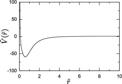
In order to connect our results to real experiments, it would be important to see the asymptotic form of the trap potential stabilizing the skyrmion. It can be analytically derived from asymptotic analysis of differential equations (15) and (16). In the generic case that the odd asymptotically reaching , respectively, as , as seen in Appendix B, the form of the trap potential can be obtained as Eqs. (72) and (73), respectively, for and . One can easily find that these equations are consistent with the result of the analytically solvable cases discussed in Ref. [13]: for and for . For , the leading terms in Eqs. (72) and (73) are both proportional to . Interestingly, the power of the leading terms is independent of . In particular, in the case shown in Fig. 8, the analytically obtained asymptotic form for , , is in good agreement with the numerical result. On the other hand, in the case of the large- side, because of the very large prefactor , the subleading term remains effective. Thus, taking into account the leading term as well as the subleading term , the analytical result for matches the numerical one very well.
There are many open problems which would deserve further study. In this paper we only discussed skyrmions in equilibrium. Dynamical aspects, such as relaxation to the skyrmion solution, are also important. The dynamical aspects would be even more crucial in possible physical realizations of our proposal. As we have shown, the potential has to be fine-tuned to allow a stable skyrmion solution. In reality, it is impossible to construct a potential with infinite precision and thus there would be some error in the potential. This would make skyrmions absent, as a stable solution in equilibrium. However, we expect that, if the actual potential is close enough to the exact one with a skyrmion solution, the skyrmion would exist as a quasi-stable state with a certain lifetime. In order to discuss the feasibility of observation of a skyrmion, we would need to estimate the lifetime of the skyrmion in the actual potential. We hope progress will be made on these problems, and also on other directions related to our study.
Acknowledgements.
This work was supported in part by 21st Century COE programs at Tokyo Institute of Technology “Nanometer-Scale Quantum Physics” and at Hokkaido University “Topological Science and Technology”, and Grant-in-Aid for Exploratory Research No. 20654030, from MEXT, Japan. A.T. was supported by JSPS. I.F.H. was supported by the NSERC of Canada.Appendix A Shooting method
In general, iterating the discretized time step based on the boundary condition, the equation of motion can be numerically solved. Based on this observation, we adopt the so-called shooting method in the numerical scheme as follows:
- 1.
Choose the initial velocity arbitrarily.
- 2.
Given the initial velocity and the initial position , solve equation of motion (17) toward .
- 3.
If the particle goes beyond the peak of the potential at , the initial velocity was too large.
- 4.
If the particle comes back without reaching the peak of the potential at , the initial velocity was too small.
In a true solution, the particle should approach asymptotically the peak of the potential as . However, the asymptotic behavior in is quite sensitive to the initial velocity, and the numerical solution departs from the peak of the potential in either way, depending on the tiny difference of order of machine precision, in the initial velocity. The sensitivity is due to the instability of the particle at the potential peak, further enhanced by the negative dissipation coefficient. On the other hand, because of this sensitivity, we can easily obtain the correct initial velocity in a high precision.
In practice, the shooting method can be implemented as an efficient iteration using the bisection method as follows:
- 1.
Find the two values of the initial velocity , so that is “too small” and is “too large.”
- 2.
On th iteration, the correct initial velocity should be within the range . Thus, numerically solve the equation of motion with the midpoint initial velocity .
- 3.
If the midpoint is too small as the initial velocity, set , , If is too large, set instead , . Go to step 2 as the th iteration.
In this way, the error in the initial velocity decreases proportionally to in the th iteration.
Appendix B Asymptotic form of trap potentials
In order to drive the asymptotic form of trap potentials, we rewrite equation of motion (17) for and . Then, in this odd-dissipation case can be approximated as for and for . In addition, as shown by the numerical results, the solution would stand near and . From these assumptions, equation of motion (17) is linearized as
| (68) |
for , and
| (69) |
for . The solutions satisfying the boundary conditions, and , can be easily obtained, respectively, as
| (70) |
where . and are unknown constants. On the other hand, from the boundary conditions for and the definition of the dissipation , the asymptotic forms of the density profile for and are easily obtained as
| (71) |
Taking asymptotic forms (70) and (71) from the representation to representation by , and substituting them into one of equations of motion (15), the trap potential can be derived. As a result, for and are investigated as
| (72) |
for , and
| (73) |
for . and are unknown constants and are the prefactors of the density profile, respectively, for and . In particular, in the case of discussed in this paper, they turn out to be appearing in Eq. (66): . The leading term is decided by the value of . However, in Fig. 8, because of the very large prefactor , the subleading term still remains effective in shown region of .
References
- [1] I. Herbut, A Modern Approach to Critical Phenomena (Cambridge University Press, Cambridge, 2007).
- [2] A. A. Belavin and A. M. Polyakov, JETP Lett. 22, 245 (1975).
- [3] N. Manton and P. Sutcliffe, Topological Solitons (Cambridge University Press, Cambridge, England, 2004).
- [4] M. H. Lau and C. Dasgupta, Phys. Rev. B 39, 7212 (1989); M. Kamal and G. Murthy, Phys. Rev. Lett. 71, 1911 (1993); N. D. Antunes, L. M. A. Bettencourt, and M. Kunz, Phys. Rev. E 65, 066117 (2002); O. I. Motrunich and A. Vishwanath, Phys. Rev. B 70, 075104 (2004).
- [5] E. Eisenberg and E. H. Lieb, Phys. Rev. Lett. 89, 220403 (2002).
- [6] A. Vilenkin and A. P. S. Shellard, Cosmic Strings and Other Topological Defects (Cambridge University Press, 1994).
- [7] For a recent review, see K. Kasamatsu, M. Tsubota, and M. Ueda, Int. J. Mod. Phys. B 19, 1835 (2005).
- [8] Y. Saiga and M. Oshikawa, Phys. Rev. Lett. 96, 036406 (2006).
- [9] I. F. Herbut, Phys. Rev. Lett. 94, 237001 (2005); 88, 047006 (2002); Phys. Rev. B 66, 094504 (2002).
- [10] M. Franz, Z. Tešanović, and O. Vafek, Phys. Rev. B 66, 054535 (2002); Z. Tešanović, Phys. Rev. Lett. 93, 217004 (2004); Nature Phys. 4, 408 (2008).
- [11] T. Senthil and M. P. A. Fisher, Phys. Rev. B 74, 064405 (2006).
- [12] G. H. Derrick, J. Math. Phys. 5, 1252 (1964).
- [13] I. F. Herbut and M. Oshikawa, Phys. Rev. Lett. 97, 080403 (2006).
- [14] See also L. Lichtensteiger and R. Durrer, Phys. Rev. D 59, 125007 (1999).
- [15] L. D. Landau and E. M. Lifshitz, Mechanics (Pergamon, Oxford, 1976), Chap. 5.