The von Neumann entropy of networks

The quantum entropy (or, equivalently, von Neumann entropy) was defined by von Neumann around 1927 for proving the irreversibility of quantum measurement processes [28]. Precisely, the quantum entropy is an extension of the Gibbs entropy to the quantum realm and it may be viewed as the average information the experimenter obtains in the repeated observations of many copies of an identically prepared mixed state. It has a fundamental role for studying correlated systems and for defining entanglement measures [29, 30]. In the present work we elaborate on the notion of quantum entropy applied to networks. Since the quantum entropy is defined for quantum states, the first required ingredient is therefore a method to map graphs/networks into states (while the converse is not necessary in our purpose). The literature comprises different ways to associate graphs to certain states or dynamics. Notably, graph-states and spin networks, just to mention two major ones: graph-states are certain quantum error correcting codes, important for characterizing the computational resources in measurement based quantum computation [6, 19]; spin networks are arrangements of interacting quantum mechanical particles, nowadays of great significance for the development of nanotechnologies [3, 4, 21]. We take a straightforward approach, and take into analysis an entropic quantity for graphs on the basis of a faithful mapping between discrete Laplacians and quantum states, firstly introduced by Braunstein et al. [5] (see also [20]). In synthesis, we see the spectrum of an appropriately normalized Laplacian as a distribution and we compute its Shannon entropy [8] (which measures the amount of uncertainty of a random variable, or the amount of information obtained when its value is revealed). Such a quantity finds a natural place among those global spectral parameters of graphs (i.e., involving the entire spectrum and not just a specific eigenvalue) studied in connection to natural and social networks. For example, the Estrada index, a measure of centrality [15], also used to quantify the degree of folding of long-chain molecules [12, 13, 24]; or the graph energy, that in Hückel theory corresponds to the sum of the energies of all the electrons in a molecule [10, 18]. (See the book chapter [7], for a general review on complexity measures for graphs.) We give evidence that the quantum entropy is a measure of regularity for graphs, i.e., regular graphs have in general higher entropy when the number of edges is fixed. Moreover, entropy seems to depend on the number of connected components, long paths, and nontrivial symmetries. Chosen the number of edges, entropy is smaller for graphs with large cliques and short paths, i.e., graphs in which the vertices form an highly connected cluster. The remainder of the paper is organized as follows. In Section II we introduce the required definitions and focus on some basic properties. By adding edges one by one to the empty graph, we try to construct graphs with minimum and maximum entropy. In Section III we explore the influence of the graph structure on the entropy. We consider different classes of graphs: regular graphs, random graphs, and the star as an extremal case of scale-free graph (i.e., graphs for which the degree distribution follows a power law). The asymptotic behavior for large number of vertices shows that regular graphs tend to have maximum entropy. We study numerically how the entropy increases when adding edges with different prescriptions. Once fixed the number of edges, the entropy is minimized by graphs with large cliques. Section IV contains remarks and open problems.

The state of a quantum mechanical system with a Hilbert space of finite dimension $n$ is described by a density matrix. Each density matrix $\rho$ is a positive semidefinite matrix with Tr$(\rho)=1$. As we have already mentioned in the introduction, there are many ways to associate graphs to specific density matrices or Hamiltonian evolution (e.g., graph states, bosonic systems, etc.). Here we consider a matrix representation based on the combinatorial Laplacian. Let $G=(V,E)$ be a simple undirected graph with set of vertices $V(G)=\{1,2,...,n\}$ and set of edges $E(G)\subseteq V(G)\times V(G)-\{\{v,v\}:v\in V(G)\}$. The adjacency matrix of $G$ is denoted by $A(G)$ and defined by $[A(G)]_{u,v}=1$ if $\{u,v\}\in E(G)$ and $[A(G)]_{u,v}=0$, otherwise. The degree of a vertex $v\in V(G)$, denoted by $d(v)$, is the number of edges adjacent to $v$. A graph $G$ is $d$-regular if $d(v)=d$ for all $v\in V(G)$. Let $d_{G}$ be the degree-sum of the graph, i.e. $d_{G}=\sum_{v\in V(G)}d(v)$. The average degree of $G$ is defined by $\bar{d}_{G}:=\tilde{n}^{-1}\sum_{v\in V(G)}d(v)$, where $\tilde{n}$ is the number of non-isolated vertices, that is vertices $v$ such that $\{u,v\}\in E(G)$ for some $u\in V(G)$. The degree matrix of $G$ is an $n\times n$ matrix, denoted by $\Delta(G)$, having $uv$-th entry defined as follows: $\left[\Delta(G)\right]_{u,v}=d(v)$ if $u=v$ and $\left[\Delta(G)\right]_{u,v}=0$, otherwise. The combinatorial Laplacian matrix of a graph $G$ (for short, Laplacian) is the matrix $L(G)=\Delta(G)-A(G)$. The matrix $L(G)$ is a major tool for enumerating spanning trees (via the Matrix-Tree Theorem) and has numerous applications (see Kirchhoff [22], Biggs [2], and Grone et al. [16, 17]). As a consequence of the Geršgorin disc theorem, $L(G)$ is positive semidefinite. By these definitions, the Laplacian of a graph $G$ scaled by the degree-sum of $G$ is a density matrix: $\rho_{G}:=\frac{L(G)}{d_{G}}=\frac{L(G)}{\text{Tr}(\Delta(G))}$. It is then clear that $\rho_{G}=\frac{L(G)}{\tilde{n}\bar{d}_{G}}$. The entropy of a density matrix $\rho$ is defined as $S(\rho)=-$Tr$(\rho\log_{2}\rho)$. Now, given the notion of Laplacian, we say that $S(\rho_{G})$ is the quantum entropy (or, for short, entropy) of $G$. Let $\nu_{1}\geq\nu_{2}\geq\cdots\geq\nu_{n}=0$ and $\lambda_{1}\geq\lambda_{2}\geq\cdots\geq\lambda_{n}=0$ be the eigenvalues of $L(G)$ and $\rho_{G}$, respectively. These are related by a scaling factor, i.e. $\lambda_{i}=\frac{\nu_{i}}{d_{G}}=\frac{\nu_{i}}{\tilde{n}\bar{d}_{G}}$, for $i=1,...,n$. The entropy of $\rho_{G}$ can be also written as $S(G)=-\sum_{i=1}^{n}\lambda_{i}\log_{2}\lambda_{i}$, where $0\log_{2}0=0$, by convention. (See [27] for a survey on Laplacian spectra.) Since its rows sum up to $0$, then $0$ is the smallest eigenvalue of $\rho_{G}$. The number of connected components of $G$ is equal to the multiplicity of $0$ as an eigenvalue. The largest Laplacian eigenvalue is bounded by the number of non-isolated vertices, i.e., $\nu_{1}\leq\tilde{n}$ (see Duval et al. [11], Proposition 6.2); thus it follows immediately that $0\leq\lambda_{i}\leq\frac{1}{\bar{d}_{G}}$, for $i=1,...,n$. It is important to remark that since $0\leq\lambda_{i}\leq\frac{1}{\bar{d}_{G}}\leq 1$, for $i=1,...,n$, $S(\rho_{G})$ equals the Shannon entropy of the probability distribution $\{\lambda_{i}\}_{i=1}^{n}$. If a general density matrix $\rho$ has an eigenvalue $1$ then the other must be $0$ and $\rho=\rho^{2}$. In such a case, the density matrix is said to be pure; otherwise, mixed. For later convenience, we define the quantity $R(G):=\frac{1}{n}\sum_{i=1}^{n}\frac{\nu_{i}}{\bar{d}_{G}}\log_{2}\frac{\nu_{i}}{\bar{d}_{G}}$. The disjoint union of graphs $G$ and $H$ is the graph $G^{\prime}=G\uplus H$, whose connected components are $G$ and $H$. We denote by $K_{n}$ the complete graph on $n$ vertices. Let $\mathcal{G}_{n}$ be the set of all graphs on $n$ vertices. The next fact was proved by Braunstein et al. [5]:

For general density matrices, $S(\rho)=0$, if $\rho$ is a pure state; $S(\rho)=-\log_{2}\frac{1}{n}=\log_{2}n$ if $\rho=\frac{1}{n}I_{n}$, i.e., a completely random state. The analogue in $\mathcal{G}_{n}$ is $K_{n}$ given that the spectrum or $\rho_{K_{n}}$ is $\{\frac{1}{n-1}^{[n-1]},0^{[1]}\}$. The next result bounds the variation of the entropy under edge addition. Let $G^{\prime}=G+\{x,y\}$, where $V(G)=V(G^{\prime})$ and $E(G^{\prime})=E(G)\cup\{u,v\}$. An alternative proof could be given by invoking eigenvalues interlacing [10].

Starting from $K_{2}\biguplus_{j}K_{1}^{(j)}$ (the graph with zero entropy) we can think of a discrete-time process in which we add edges so that the entropy is extremal (resp. maximum or minimum) at every step. Let us denote by $G_{i}^{\max}$ and $G_{i}^{\min}$, $i\geq 1$, the graphs with maximum and minimum entropy at the $i$-th step, respectively. Figure 1 contains $S(G_{i}^{\max})$ and $S(G_{i}^{\min})$ (resp. solid and dashed line) as functions of the number of edges $i=1,2,...,15$, for graphs in $\mathcal{G}_{6}$. The initial graph is $G_{1}^{\max}=G_{1}^{\min}=K_{2}\biguplus_{j=3}^{6}K_{1}^{(j)}$; the final one is $G_{15}^{\max}=G_{15}^{\min}=K_{6}$. Each edge labeled by $j\leq i$ in the graph $K_{6}$ on the left (resp. right) hand side of Figure 2 is also an edge of $G_{i}^{\max}$ (resp. $G_{i}^{\min}$). This illustrates the steps for constructing every $G_{i}^{\max}$ and $G_{i}^{\min}$. It turns out that the vertices of $G_{i}^{\max}$ tend to have “almost equal” or equal degree. In fact $G_{i}^{\max}$ is a $i/3$-regular graph, for $i=3,6,9,12$. On the other hand, $G_{l(l-1)/2}^{\min}=K_{l}\biguplus_{j=1}^{6-l}K_{1}^{(j)}$, if $l=3,4,5$. The meaning is without ambiguity: entropy is minimized by those graphs with locally added edges, i.e. edges increasing the number of complete subgraphs (also called cliques). Even if we consider graphs with only six vertices, it is already evident that long paths, nontrivial symmetries and connected components give rise to a larger increase of the entropy. This property is confirmed by further numerical analysis in the next section.

Let $\mathcal{G}_{n,d}$ be the set of all $d$-regular graphs. For $G\in\mathcal{G}_{n,d}$, we have $\Delta(G)=dI_{n}$, and hence $\lambda_{i}=\frac{d-\mu_{i}}{\text{Tr}\left(\Delta(G)\right)}=\frac{d-\mu_{i}}{dn}$, for $i=1,2,...,n$, where $\mu_{i}$ denotes the $i$-th eigenvalue of $A(G)$.

It may useful to remark two points: (1) The simplest regular graph is the perfect matching $M_{n}:=\biguplus_{j=1}^{n/2}K_{2}^{(j)}$. The density matrix of $M_{n}$ is then $\rho_{M_{n}}=\frac{1}{n}\bigoplus\nolimits_{n/2\text{ times}}\left(\begin{array}[c]{rr}1&-1\\ -1&1\end{array}\right)$ and $S(M_{n})=-\frac{n}{2}\left(\frac{2}{n}\log_{2}\frac{2}{n}\right)=\log_{2}\frac{n}{2}$, because $\lambda_{1}^{[\frac{n}{2}]}=\frac{n}{2}$ and $\lambda_{2}^{[\frac{n}{2}]}=0$. Thus, $S(M_{n})=S(K_{n/2+1})$. For $M_{4}$ we have $S(M_{4})=S(K_{3})=1$. More generally, $S\left(M_{2^{k}}\right)=k-1$. (2) The entropy of $G\in\mathcal{G}_{n\rightarrow\infty}$ tends to the entropy of $K_{n}$ if all the quantities $\frac{\nu_{i}}{\bar{d}_{G}}$ remain finite, i.e., $\lim_{n\rightarrow\infty}\frac{R(G)}{\log_{2}n}=0$.

The complete bipartite graph $K_{p,q}$ has $V(K_{p,q})=A\cup B$, where $\left|A\right|=p$ and $\left|B\right|=q$, and each vertex in $A$ is adjacent to every vertex in $B$. The graph $K_{1,n-1}$ on $n$ vertices is said to be a star.

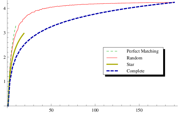
Similarly to what we have done in the previous section, we observe how the entropy of a graph $G\in\mathcal{G}_{n}$ increases as a function of $\left|E(G)\right|=e$. Starting from $K_{2}\biguplus_{j=1}^{n-2}K_{1}^{(j)}$, we consider four different ways of adding edges: (i) Random graphs with exactly $e$ edges. These are constructed by chosing $e$ pairs of vertices at random from the total number of pairs; (ii) The graph $M_{2e}\biguplus_{j=1}^{n-2e}K_{1}^{(j)}$; (iii) The graph $K_{1,(e+1)-1}\biguplus_{j=1}^{n-e-1}K_{1}^{(j)}$; (iv) The graph $K_{m}\biguplus_{j=1}^{n-m}K_{1}^{(j)}$, where $m=\left[\frac{1+\sqrt{1+8e}}{2}\right]$. Recall that adding isolated vertices to a graph does not change its entropy. Figure 3 shows the case $n=20$. It is evident that the entropy is larger for graphs with an high number of connected components. In this sense, $M_{n}$ has relatively high entropy. The smallest entropy is obtained for complete graphs.

Next is a list of remarks and open problems:

We conclude with two open problems: does the star $K_{1,n-1}$ have smallest entropy among all connected graphs on $n$ vertices? Is the entropy strictly monotonically increasing under edge addition?

References

- [1] G. Bianconi, The entropy of network ensembles. arXiv:0802.2888v2 [cond-mat.dis-nn]
- [2] N. Biggs, Algebraic Graph Theory, Cambridge, UK: Cambridge University Press, 1993.
- [3] B. B. Blinov, D. L. Moehring, L.-M. Duan, and C. Monroe, Nature 428, 153 (2004).
- [4] S. Bose, Contemporary Physics, Vol. 48 (1), pp. 13-30, 2007. arXiv:0802.1224v1 [cond-mat.other]
- [5] S. Braunstein, S. Ghosh, S. Severini, The laplacian of a graph as a density matrix: a basic combinatorial approach to separability of mixed states, Ann. of Combinatorics, 10, no 3 (2006), 291-317.
- [6] H.-J. Briegel and R. Raussendorf, Phys. Rev. Lett. 86, 910 (2001).
- [7] D. Bonchev and G. A. Buck, Quantitative Measures of Network Complexity. In: Complexity in Chemistry, Biology and Ecology, D. Bonchev and D. H. Rouvray, Eds., Springer, New York, 2005, p. 191-235.
- [8] T. Cover and J. Thomas, Elements of information theory, John Wiley, New York, 1991.
- [9] F. R. K. Chung, Spectral graph theory, CBMS Regional Conference Series in Mathematics, 92. Published for the Conference Board of the Mathematical Sciences, Washington, DC; by the American Mathematical Society, Providence, RI, 1997.
- [10] D. M. Cvetkovic, M. Doob, H. Sachs, Spectra of graph theory and applications, VEB Deutscher Berlin, Academic Press, New York, 1979.
- [11] A. M. Duval and V. Reiner, Shifted simplicial complexes are Laplacian integral, Trans. Amer. Math. Soc., 354(11):4313-4344, 2002.
- [12] E. Estrada, Characterization of the folding degree of proteins, Bioinformatics 18 (2002), pp. 697–704.
- [13] E. Estrada and J. A. Rodríguez-Velázquez, Subgraph centrality in complex networks, Phys. Rev. E 71 (2005), 1-9.
- [14] M. Fiedler, Algebraic connectivity of graphs, Czechoslovak Mathematics Journal, 23:298-305, 1973.
- [15] L. C. Freeman, A set of measures of centrality based on betweenness, Sociometry, 40, 35–41 (1977).
- [16] R. Grone, R. Merris, V. Sunder, The Laplacian spectrum of a graph, SIAM J. Matrix Anal. Appl. 11 (1990), 218–238.
- [17] R. Grone, R. Merris, The Laplacian spectrum of a graph, II. SIAM J. Discrete Math. 7 (1994), no. 2, 221–229.
- [18] I. Gutman, The energy of a graph, Ber. Math. Stat. Sekt. Forschungszentrum Graz., 103: 1-22 (1978).
- [19] M. Hein, J. Eisert, and H.J. Briegel. Multi-party entanglement in graph states, Phys. Rev. A 69, 062311 (2004).
- [20] R. Hildebrand, S. Mancini, S. Severini, Combinatorial laplacians and positivity under partial transpose, Math. Struct. in Comp. Science (2008), 18, 205–219.
- [21] D. Kielpinski, C. Monroe, and D. J. Wineland, Nature 417, 709 (2002).
- [22] F. Kirchhoff, Über die Auflösung der Gleichungen, auf welche man bei der Untersuchung der linearen Verteilung galvanischer Ströme gef¨uhrt wird. Ann. Phys. Chem. 72 (1847), 497—508.
- [23] J. Körner, Coding of an information source having ambiguous alphabet and entropy of graphs, In Proc. 6th Prague Conference on Information Theory (1973), pp. 411–425.
- [24] M. Lazić, On the Laplacian energy of a graph, Czechoslovak Math. J. 56(131) (2006), no. 4, 1207–1213.
- [25] H. H. Lieb, M. B. Ruskai, Proof of the strong subadditivity of quantum-mechanical entropy, J. Math. Phys. 14, 1938–1941 (1973).
- [26] L. Lovász, Random walks on graphs: a survey. Combinatorics, Paul Erdős is eighty, Vol. 2 (Keszthely, 1993), 353–397, Bolyai Soc. Math. Stud., 2, János Bolyai Math. Soc., Budapest, 1996.
- [27] B. Mohar, The Laplacian spectrum of graphs. Graph Theory, Combinatorics, and Applications, 2:871-898, 1991.
- [28] J. von Neumann, Mathematische Grundlagen der Quantenmechanik, Berlin, 1932; English translation by R. T. Beyer, Mathematical Foundations of Quantum Mechanics, Princeton, 1955.
- [29] M. A. Nielsen and I. L. Chuang, Quantum computation and quantum information, Cambridge University Press, Cambridge, 2000.
- [30] M. Ohya, D. Petz, Quantum entropy and its use. Texts and Monographs in Physics. Springer-Verlag, Berlin, 1993.
- [31] S. Riis, Graph Entropy, Network Coding and Guessing games. arXiv:0711.4175v1 [math.CO]
- [32] G. Simonyi, Graph entropy. In Combinatorial Optimization, L. L. W. Cook and P. Seymour, Eds., vol. 20 of DIMACS Series on Discrete Math and Computer Science. 1995, pp. 391–441.
- [33] A. Terras, Fourier analysis on finite groups and applications, London Mathematical Society Student Texts, 43. Cambridge University Press, Cambridge (1999).
- [34] V. Vedral, The role of relative entropy in quantum information theory, Reviews of Modern Physics, vol. 74, Issue 1, pp. 197-234.