Report: IFIC/08-61, FTUV-08-1212
Prospects of searching for (un)particles from Hidden Sectors
using rapidity correlations in multiparticle production at the LHC
Miguel-Angel Sanchis-Lozano 11 1 Email:Miguel.Angel.Sanchis@ific.uv.es
Instituto de Física
Corpuscular (IFIC) and Departamento de Física Teórica
Centro Mixto Universitat de València-CSIC,
Dr. Moliner 50, E-46100 Burjassot, Valencia (Spain)
Most signatures of new physics have been studied on the
transverse plane with respect to the beam direction
at the LHC where background is much reduced.
In this paper we propose
the analysis of inclusive longitudinal (pseudo)rapidity correlations
among final-state (charged) particles in order to search
for (un)particles belonging to a Hidden Sector
beyond the Standard Model, using a selected sample of p-p minimum bias events
(applying appropriate off-line cuts on events based on, e.g.,
minijets, high-multiplicity, event shape variables, high- leptons
and photons, etc) collected at the early running of the LHC.
To this aim,
we examine inclusive and semi-inclusive two-particle
correlation functions, forward-backward correlations, and
factorial moments of the multiplicity distribution,
without resorting to any particular model but
under very general (though simplifying) assumptions. Finally, motivated by
some analysis techniques employed in the search for Quark-Gluon-Plasma
in heavy-ion collisions, we
investigate the impact of such intermediate (un)particle stuff
on the (multi)fractality of parton cascades in p-p collisions,
by means of a Lévy stable law description and a
Ginzburg-Landau model of phase transitions. Results from our
preliminary study seem encouraging for possible dedicated
analyses at LHC and Tevatron experiments.
1 Introduction
Most signatures and signals of new phenomena are expected to be found in hard events at the LHC on the transverse plane with respect to the beam direction where new physics (NP) would show up while background is much reduced. Typical examples for direct discovery” are high- jets, large missing , large invariant mass of dileptons, diphotons or dijets, high-energy monochromatic photons, etc (see e.g. [1] and references therein). However, a proposal has been put forward recently [2] to search for new physics in anomalous underlying events, looking for soft diffuse signals in the tracking system and calorimetry of the LHC experiments. Earlier, possible signals of NP from global event properties (notably manifesting in the tail of the charged particle multiplicity distribution) were studied in [3].
In this paper we propose to the CERN LHC collaborations [4, 5] to consider further signatures of NP in multiparticle production, by carefully scrutinizing inclusive (longitudinal) rapidity correlations between (charged) particles emitted in inelastic proton-proton (p-p) interactions. We are particularly interested in (un)particles from a Hidden Sector (HS) beyond the Standard Model (SM) (sometimes more generally -and thought-provokingly- described as hidden worlds” [6]) contributing through a new state of matter to the hadronization chain yielding final-state SM particles. Our approach does not rely on any particular model, besides some general (but simplifying) assumptions on hadroproduction, and should be considered as a starting point for a much more complete study.
The study of inclusive densities of secondaries and correlations between them has indeed been providing for decades (in cosmic rays physics, fixed target and collider experiments) extremely useful information about the strong interaction dynamics in high-energy interactions. Notably, high-order correlations among emitted particles have been found in all types of hadron collisions, manifesting through multiplicity fluctuations when phase-space is split in small cells. The normalized moments of the multiplicity distributions then exhibit a power-law dependence (intermittency”), analogous to that observed in other (multi)fractal phenomena in Nature, like galaxy clustering [7]. Besides, particle correlations provide essential information on the properties of jets, with the advantage that the systematic error due to missing particles in the jet is not so relevant as in other observables as stressed in [8]. Actually, particle production inside QCD jets follows a self-similar multifractal pattern, as could be expected from a multiplicative branching process.
In this work we argue that an extra non-standard state of matter at the onset of the parton cascade might significantly change its multifractality character, advocating the use of estimators to determine the mono- or multi-fractal character of the hadroproduction process. A suggestive connection will be established between our prospects of looking for hidden (un)particles in p-p collisions, and the formation of quark-gluon plasma in heavy-ion collisions, where a Lévy stable law description and a Ginzburg-Landau model of phase transitions have been thoroughly applied to study the deconfinement phase transition [9].
The layout of the paper is as follows. In section 2 we present a survey on multibody production in inelastic p-p collisions, where widely used concepts and tools particularly important for our proposal are highlighted. Hidden sectors (Unparticle, Hidden Valley, and other scenarios like Technicolor, Quirks or even mini Black Holes) are very briefly addressed in section 3 regarding the phenomenology at hadron colliders. In section 4 we introduce our notation and basic formulas for the inclusive analysis. Cascades in hadronic collisions are considered in section 5 under the working hypotheses of two- and three-step scenarios, studying the effect on the correlation functions and moments of the multiplicity distribution. Section 6 is devoted to the study of Forward-Backward correlations. Intermittency and (multi)fractality are examined in section 7 working out an illustrative exercise” largely motivated by usual analyses of heavy-ion collisions. Finally, a summary and a short proposal for this kind of analysis at the LHC are given in section 8.
2 A short survey on multiparticle dynamics
Experimental results in multibody hadroproduction collected along decades have steadily supported the tendency of produced particles to merge into correlated groups [10]. This experimental evidence rapidly led to the view of a two-step process for high-energy hadron collisions: More or less well-defined hadronic objects should emerge during the first stage of the interaction, subsequently decaying into final-state particles through a complicated and, to a large extent, non-perturbative shower. In the following 22 2 This section can be skipped by the reader already familiar with the topic., we highlight basic points of multiparticle dynamics, not in a comprehensive way at all, but focusing on those aspects especially related to our suggestion.
2.1 Early models
The statistical approach to multiparticle production was first independently proposed by Fermi and Wilson in the fifties [11, 12]. In this model, the energy of the collision concentrates in a small interaction volume where various kinds of particles, mainly pions, are created. A statistical equilibrium was assumed to be reached in the gas” of such confined particles. The effect of strong interaction in the original Fermi model was restricted to establish some sort of statistical equilibrium. Limited progress of this picture was performed by Landau [13] in the hydrodynamical model for hadroproduction.
In the Fermi model, the strong interaction played only a marginal role, defining to some extent the radius of the initial volume. Strong interactions were taken more seriously into account by Hagedorn in the statistical bootstrap model [14] whereby resonance-like structures (fireballs) emerged: a fireball consisted of fireballs, in turn consisting of fireballs, and so on till the hadronization stage. The hadronic excitation spectrum was also later derived in the dual resonance model [15]. With the advent of the quark model of hadrons and Quantum Chromodynamics, it became clear that the fireball’s temperature was in fact a transition point to a new state of matter in heavy-ion collisions, a plasma of deconfined quarks and gluons [16]. On the other hand, a short-coming of the statistical model was the isotropy in the decays being at odds of the observed anisotropic angular distributions from cosmic ray collisions. To explain this discrepancy, a two-fireball model was put forward, where both fireballs could move according to an empirical velocity distribution to be determined from experimental fits.
Further developments arose in the sixties extending the original Yukawa’s idea on the exchange of pions among nucleons to further explain the strong interaction between hadrons in scattering processes. In accordance with the copious pionization and dominance of short-range correlations, the multiperipheral model [17] of hadron inelastic collisions assumed that virtual hadronic objects exchanged between colliding hadrons (pions, Regge trajectories, Pomerons…) could themselves radiate groups of correlated secondaries providing a theoretical motivation for clusters of particles [18]. Clustering of final-state particles has been indeed experimentally confirmed in many multi-particle processes but cannot be entirely identified with low-mass resonances (, ,…) (see e.g. [19, 20]).
It was quickly recognized, moreover, that the decays of two or more clusters in an event could easily overlap in (pseudo)rapidity 33 3 The longitudinal rapidity of a particle is defined as where and denotes respectively the energy and longitudinal momentum along the beam direction. Experimentally it becomes customary to measure a closely related variable, the pseudorapidity, defined as where denotes the particle momentum; rapidity and pseudorapidity coincide as far as , i.e. when the particle mass is negligible as compared to the transverse momentum. This is generally the case for most secondaries (mostly pions) in a high-energy inelastic collision. From an experimental point of view, the pseudorapidity can be obtained directly from the measurement of the polar angle of the emitted particle with respect to the beam direction: ., rendering the assignment of particles to one or another cluster an almost impossible task. Actually, the question arises whether such clusters are real hadronic objects or purely statistical artefacts to describe probability distributions for high-energy multiparticle collisions.
Recently, following the Feynman gas picture [12, 21], a semi-empirical formula based on the formation and decay of two cylinders” has been formulated to account for the (pseudo)rapidity distributions of charged particles in hadronic inelastic collisions [22]. At high enough energy, both projectile and target cylinders are expected to overlap only partially, developing a rapidity gap between both fragmentation regions. Linear relationships between the width of charged (pseudo)rapidity density distributions and are found, in good agreement with experimental data for p-p and nucleus-nucleus (A-A) collisions. Moreover, multiplicity distributions in proton and heavy-ion collisions can be included in a unified description where particles are emitted from clusters formed at the collision [23].
2.2 Inclusive analysis: limiting fragmentation and plateau rise
Investigations of multiparticle production basically rely upon experimental results on: total cross sections, multiplicity distributions, transverse momentum and single-particle inclusive rapidity distributions, two-, three-, or many-particle correlations, azimuthal correlations, etc. Because of the huge amount of particles produced in hadronic collisions at high energy, and the obvious experimental difficulty for complete detection, inclusive analyses of events prove indeed to be extremely useful.
As usual, by one-particle (two-particle) inclusive process we understand a reaction such that
| (1) |
where () denote(s) here one (two) charged particle(s) and is an unknown system of particles. At LHC energies most of the emitted charged particles will be pions.
Feynman in 1969 gave a description of hadronic interactions leading to the conclusion that as ( is the center-of-mass energy) the inclusive cross section, expressed in terms of and , where ()is the momentum parallel (transverse) to the incident direction of the outgoing particle in the center-of-mass system (c.m.s.) of the collision, becomes independent of the energy:
| (2) |
More or less at the same time, Yang and collaborators [24] from a rather different point of view suggested the hypothesis of limiting fragmentation whereby at high enough energies the inclusive cross section for the production of particle from a target (or projectile) should be independent of the incident energy and type of the other collision partner [25]. For away from , these two kinds of scaling are equivalent, while at Feynman scaling implies that the inclusive rapidity distribution develops a constant (i.e. -independent) plateau (see Fig.1).

When expressed in terms of the rapidity variable, limiting fragmentation requires the correlation length hypothesis which states that there is no correlation between particles whose rapidities differ by more than a certain correlation length 44 4 There is no compelling reason for a unique correlation length but we will use one symbol for simplicity. ; that is for . Moreover, there is no correlation with the colliding particles as long as their rapidities and differ from by a distance large compared to . Therefore, considering a single-particle spectrum, whose maximum length 55 5 The total length of the rapidity plot is sometimes defined by the rapidities of the colliding particles , sometimes as where is the pion mass. The latter choice means that and are not exactly at the ends of the rapidity plots. In practice, the difference is insubstantial. will be denoted by , three regions can be distinguished [17] in the c.m.s.: a) Target fragmentation region, where ; b) Central region, where and the aforementioned plateau rises; c) Projectile fragmentation region, where .
Obviously at hadron colliders there is a symmetrical situation regarding both target and projectile regions, potentially useful for determining systematic uncertainties in inclusive analyses. At LHC energies ; however, we will implicitly restrict our study throughout this paper to the central region . Notice that a distorsion (dip) is introduced in the central plateau whenever the pseudorapidity variable is used in lieu of the rapidity.
The early and naive expectation that the rapidity density (i.e. the height of the plateau) would be independent of , and that the plateau would merely widen as the energy is increased, leading to a logarithmic growth of multiplicity [12], is clearly not in accord with data. It rather turns out that the total (charged) multiplicity grows as [26] (see [27, 28] for a discussion on the dissipating/effective energy in the collision). This fact can be seen as a phenomenological consequence of three concurrent features: a) The increase as of the particle density at midrapidity, b) The almost trapezoidal shape (see Fig.1) of the (pseudo)rapidity distribution, and c) the growth of the width of the spectrum proportional to . Let us note that the predicted density in the central region at LHC energies lies between 6 and 8 charged particles per rapidity unit, depending on the MC generator and model [29, 30].
Experimental data indeed have shown that Feynman scaling does not hold for the low (central) region, but limiting fragmentation does. In fact, it turns out that limiting fragmentation extends to a much wider range of rapidities than originally thought, while the width of the central plateau grows much slower than initially anticipated. According to Ref.[31], these features can be understood from a two-step process in hadron collisions where the key-point is the flat distributions (in rapidity) of both radiating partons and clusters in the string decay.
Still the dynamical origin of the rise with energy of the central plateau is not known though different models can account for it. For example, it has been argued in [32] about two possible causes, namely: a) increasing overlap in rapidity space of the fragmenting valence-quark chains, b) contribution from additional chains. This interpretation is supported by the experimental observation that the plateau rise is mainly originated from the small- region. Finally, let us point out that is remarkably independent of for low multiplicities, while exhibits a considerable increase for high multiplicity events (see [33, 34] for a general review on hadron collisions with references therein).
2.3 Multiplicity distributions
Another important result to understand multibody dynamics is the shape of the (charged) multiplicity distribution, . In 1972 Koba, Nielson and Olesen [35] proposed that the function
| (3) |
should become asymptotically independent of , where is the average number of (charged) particles per event, and denote the cross section for production of charged particles and total inelastic cross section, respectively. In other words, according to the KNO hypothesis the multiplicity distribution for a given type of reaction depends only on the ratio of the number of particles to the average multiplicity. Note that exact KNO scaling implies that particle correlations in general, and the normalized moments of the multiplicity distribution in particular: , are independent of in contradiction with experimental observation [36, 34].
In fact KNO scaling was approximately observed up to ISR energies in p-p collisions. However, as the c.m.s. energy increases, the multiplicity distribution becomes broader, developing a shoulder” structure at high , hence breaking KNO scaling [37]. Such a shoulder is usually ascribed to the multi-source nature of the processes, either from additional ladders, multi-parton interactions, or the presence of two components in events: one related to the conventional soft interaction, the other to QCD minijets. It is relevant to point out here a generalization of KNO-scaling (log-KNO) [38] (based on Polyakov’s original idea [39]) which naturally arises for self-similar multiplicative cascades. Any possible breaking of log-KNO scaling at the LHC would be a hint of a different behaviour of the parton cascade, deserving attention in our proposal.
On the other hand, the negative binomial distribution (NBD) has been extensively used to describe empirically the multiplicity distributions in almost all inelastic, high energy processes. It is given by
| (4) |
where is an adjustable parameter describing the shape of the distribution [40]; the variance can be written as: . Thus, the NBD is broader than the Poisson distribution provided that is positive and finite (corresponding to positive correlations among particles), becoming Poissonian when . The Bose-Einstein distribution is a special case of NBD with . If is negative, the NBD becomes a positive binomial distribution, narrower than Poisson (corresponding to negative correlations).
Actually, the NBD does not provide a good description of particle correlations but a of convolution of different NBD’s are required to fit experimental data [41, 42]. Nonetheless, the wide occurrence of the NBD in different types of high-energy collisions, suggested the interpretation of such distribution law in terms of clans [43] (see [44] for a review). The clan concept generalizes the jet concept: all multiplicity correlations among particle are exhausted within each clan. The new proposed parameters are the average number of groups of particles with a common ancestor denoted here as , and the average number of particles per clan, . These parameters are related to the standard ones by: and , where can be interpreted as a determination of the aggregation of partons into clusters/clans. Recently [45], the parameter has been related to a phase transition at parton level implying a discontinuity in the average number of hadrons in high-energy hadronic collisions.
2.4 Hadron-hadron versus collisions
Multiparticle production in hadron interactions might look at first glance as completely different from initiated processes. In the latter case, one expects at tree level highly virtual timelike partons. On the contrary, one generally describes a hadron-initiated process as ladders of multiperipheral-type graphs between participating constituents with low space-like virtualities. Nevertheless, a more unified picture emerges when one considers that strings stretched between colour charges may fragment yielding final particles through an intermediate clusterization stage (see for example [47, 48]).
In fact, one striking feature of multiparticle production is simplicity and universality [26, 34, 49]. For example, nuclear effects” in h-A high-energy collisions are not really nuclear but generated by the QCD partonic medium to a large extent [50]. Indeed p-p, p-A and A-A collisions were studied in [27] providing a universal production mechanism based on dissipating energy participants” in a Landau hydrodynamical model [13]. Nevertheless, similarity between different types of high-energy collisions may be more qualitative than quantitative as stressed in [51].
Current models of high-energy hadron collisions combine both perturbative QCD whenever applicable (high scattering) and a phenomenological approach to describe soft physics. Frequently employed, local parton-hadron duality implies the proportionality of inclusive distributions, becoming asymptotically correct at ultrahigh energy, thus expectedly at the LHC. (Notice however possible problems at low [52].) Actually, the subdivision of inelastic hadronic collisions into soft and hard processes is rather artificial, with semi-hard processes as a clear argument. In fact it is difficult to find a model with the right mixture of both components. In general, soft production processes are so unavoidably complex that a sophisticated approach is definitely required [53, 54] implemented in Monte Carlo generators.
In the Dual Parton Model [32] soft and semi-hard particle production in p-p inelastic collisions are understood as a multiple Pomeron exchange between interacting partons giving rise to sea-quark multi-chains which in turn fragment into final-state hadrons. According to a widely accepted picture, colour-strings are stretched between participating partons, acting as sources of particles successively broken by the creation of pairs from the sea. The most common parton subcollisions are subsequently yielding two strings between the hadrons remnants. Initial state radiation can give extra gluons contributing to the activity of the event.
The Lund model [55] deals with string fragmentation and cascades based on linear QCD confinement of quarks as the starting point and colour field breaking-up. Several Monte Carlo generators (PYTHIA, FRITIOF, etc) implement this model with further assumptions for hadronization at the final stage. In PYTHIA [56], the perturbative approach expected to be valid at high- is extended down to the low- regime, where a cutoff is required. Decreasing implies increasing the number of parton-parton interactions, ultimately leading to unitarity violation. A picture based on multiparton interaction (let us recall KNO breakdown) has been proposed to solve this problem.
On the other hand, assuming that pairwise parton interactions take place independently of each other, the number of interactions (thereby the number of strings/clusters emerging from them) in an event should obey a Poissonian distribution. However, since hadrons are also extended objects, collisions may vary over a range of impact parameters from very central to rather peripheral ones, yielding extra correlations among secondaries. One net effect is a widening of the Poissonian distribution.
In sum, all the above-mentioned frameworks (see also [57, 58] for other approaches) cope with the complexity of hadron dynamics by invoking in essence a two-step scenario; the resulting multiplicity distribution is given by the convolution of the distribution for particle emission sources (strings, clusters/clans, fireballs or whatever) with the decay/fragmentation distribution of the sources. This is basically the approach followed in this work considering a prior stage in the cascade stemming from a HS, leading to a three-step scenario provided that the parton-parton collision is hard enough.
2.5 Quark-Gluon Plasma
In ultra-relativistic heavy-ion collisions, the energies of the colliding particles are converted into thermal energy. A hot state of matter, known as quark gluon plasma (QGP), should emerge if the energy density is large enough. As the plasma expands it cools down, undergoing a phase transition from deconfined QGP to confined hadrons. Strongly interacting dense matter has been created in A-A collisions at Brookhaven RHIC [59] and will be soon further studied at CERN ALICE experiment [5].
A traditional signal sensitive to deconfinement has been the expected suppression of production in nuclear reactions [60, 61], compared to the rates extrapolated from p-p data. More generally, different signatures for QGP can be roughly divided into two groups [62]:
- •
Modifications of specific properties of particles. RHIC has in fact provided evidence for the creation of a new state of thermalized matter exhibiting almost ideal hydrodynamical behaviour based, among others, on the following facts in addition to charmonium suppression: strong jet quenching (implying an important parton energy loss in the medium ), strong elliptic flow (a signal of early thermalization and a very low viscosity of the medium), direct photon emission…
- •
Consistency of bulk properties with QGP formation, e.g. entropy growth and behaviour of thermodynamic variables, correlations and fluctuations of the particle number [63, 64, 65, 66], etc. Note that the correlation lengths can be good indicators for a phase transition. Results from two-particle correlations observed at RHIC [67] have recently been extrapolated to the LHC energy regime with a special interest in jet studies [68].
Even though the postulated extra stage from a HS in the parton shower of p-p collisions is conceptually completely different from QGP, we will still find suggestive analogies between both in our study of dynamical fluctuations and correlations in particle emission. In fact, long-distance effects in (pseudo)rapidity could become a distinctive signature of a non-standard parton cascade, as later argued. Nevertheless, studies based on a description of inelastic hadronic interactions based on the Color Glass Condensate (CGC) [69] also predict long-distance correlations [70, 65]. It is thus crucial to discriminate between those different sources of long-distance correlation effects if NP effects were claimed to be observed in this way.
2.6 Glasma
Understanding thermalization of the medium in heavy-ion collisions yielding QGP is a still open problem in the field as stressed in [71]. According to the picture presented in [72], almost instantaneously after the collision an ensemble of flux tubes of rapidity-independent color electric and magnetic fields (the Glasma) is generated, decaying into quarks and gluons eventually evolving into QGP. Particles would be produced isotropically and with equal probability along the length of such Glasma tubes spanning over large distances in rapidity, of order , where denotes the momentum saturation of partons in the nucleon wavefunction. Notice that hadronization models inspired in string fragmentation (mentioned in section 2.4 regarding the Lund model) also provide LRC due to impact parameter fluctuations. However, one peculiar new feature of Glasma is related to fields localized in the transverse scale over distances smaller than the nucleon size.
Experimentally, STAR has found LRC in heavy-ion collisions at RHIC [73], especially at large centrality (implying a larger number of participants), likely larger than can be expected from impact parameter fluctuations. Plotting the correlation strength versus the particles azimuthal angle, a structure elongated in rapidity and collimated in angle appears which can be interpreted in the Glasma framework [74]. Let us remark that these features of the ridge events are not seen in proton-proton or deuteron-gold interactions and seem to be unique to nucleus-nucleus collisions.
2.7 Minimum bias, underlying events and jets at the LHC
It is well known that high energy hadronic interactions are dominated by the production of a large number of particles with small transverse momentum , leading to the apparently striking conclusion that such collisions, governed by the strong-interaction, generally are rather soft”. As in all previous hadron colliders, soft interactions will still be the dominant processes at the LHC, and a lot of potentially interesting information to be obtained from them on hadron dynamics and new phenomena should not be overlooked. Notice, in particular, that as most of the produced particles will have low transverse momenta, dynamical correlations should show up in the longitudinal phase space.
A minimum bias event (MBE) corresponds ideally to a totally inclusive trigger and can be basically identified with a non-diffractive interaction. In practice, experiments at colliders define their own minimum bias triggers which, however, are not in essence too different among themselves. MBE’s are dominated by soft interactions, although there is also some contribution from (semi)hard parton scattering often yielding (mini)jets in the final-state.
Experimentally, data show a strong correlation among the charged particles indicating jet structure” in MBE’s even for momenta as low as 1 GeV. Let us stress, however, that it is not straightforward to extrapolate what has been learned about MBE’s, e.g., at the Tevatron to the LHC, though one could expect MBE to have harder scattering at higher energies [75].
Even though not completely clean from a theoretical viewpoint, a third category of events is generally reported in high-energy hadron collisions: semi-hard events. A semi-hard event, roughly speaking, is characterized by the presence of minijets and does not plainly fall into the soft and hard categories. Semi-hard events are likely called to play a role of utmost importance in our proposal.
On the other hand, the concept of underlying event (UE) in a hard scattering process has become nowadays an important issue in collider physics [29]. In a few words, an UE is everything but the outgoing hard jets, i.e. the event activity remaining once the jets have been removed. As hard collisions are correlated, UE and MBE do not coincide. In fact, an UE contains both soft and hard interactions: the former mainly corresponds to the beam-beam remnant interactions, while the hard component should be ascribed to the initial and final-state radiation, from colour strings stretching between the UE and the jets and from secondary parton interactions.
Usually, it has been thought of collecting MBE’s as important for the general study of general features of p-p interactions. Let us summarize below some of the main points aimed by the study of minimum and underlying events:
- •
(Re)tuning of MC generators to describe hadronic interactions [76], allowing a better understanding of systematic uncertainties. Multiparticle production should also serve as an important tool for the calibration and understanding of detectors, establishing a solid basis for exclusive channels.
- •
Better knowledge of multiparton interactions, particularly the interplay between minimum bias and underlying events, allowing a better understanding of the structure of the proton at low-. This in turn will facilitate a better control of jet backgrounds to SM and BSM physics processes.
- •
Reference study for heavy-ion collisions.
Let us add tentatively a new item to the above list: In our proposal, soft events with a (semi)hard signature tagging NP (possibly a kind of anomalous underlying event as pointed out in [2]) will play an important role in the search strategy for a HS showing up in the parton cascade.
3 Hidden sectors
3.1 Unparticle stuff
Recently, Georgi [77] introduced the notion of unparticle stuff, , based on the possibility of a scale invariant HS, with experimental signals radically different from the SM sector. Conformal invariance dictates the form of the propagator, thereby determining the virtual unparticle contributions. The unparticle stuff may appear as a non-integer number of invisible particles, . Actually unparticle does not have a fixed invariant mass; from a quantum field framework it can be seen to exhibit a continuous mass spectrum. Upon measurement, however, unparticle would behave as an ordinary particle with a definite (but arbitrary!) mass [78].
If unparticle stuff couples to the SM Higgs boson, electroweak symmetry breaking should break conformal invariance too, providing an effective mass in the unparticle propagator. Thus unparticle physics could be probed for energies together with the discovery of the Higgs boson [79, 80], typically in the window between 10 GeV and 1 TeV, i.e. at LHC reach. Moreover, interactions can effectively induce a mass gap for the unparticle sector [81] sharing common features with Hidden Valley models to be examined next. Finally note that unparticle physics also provides dark matter candidates [82, 80] with astrophysical and cosmological implications [83].
It is widely accepted that unparticle stuff could manifest itself basically in two kinds of processes:
- a)
Virtual effects, e.g., the unparticle propagator mediates processes like or , or can in loop processes, leading to new signals at colliders in precision measurements [84].
- b)
Real production of unparticle stuff, implying a new phenomenology in collider physics. The most interesting signature would be peculiar missing energy distributions because of the non-integral values of . However, it has been argued [85] that such signals may be less striking than originally advocated. Nevertheless, unparticles might travel a macroscopic distance before decaying, leading to delayed signals and displaced vertices.
Moreover, in Ref.[86] unparticle self-interaction is considered as mediating processes such as , i.e. with two or more unparticles in the final-state. It is phenomenologically interesting to realize that, conversely to SM channels such as , the creation of additional unparticles in the final-state does not suppress the rate of multi-unparticle production, for strongly-coupled conformal sectors. This feature is especially relevant for our proposal because of the fluctuations of the number of intermediate states in the hadronization process, though the requirement of converting back to SM particles may imply that they are sub-dominant.
As previously commented, missing energy and momentum carried away by the unparticle have been claimed as typical signatures, pretty much as for Kaluza-Klein modes in a large extra dimension scenario. Several processes have been then envisaged based on real emission of unparticle stuff: , Higgs , quarkonium , etc (see [87] for a minireview).
However, unparticle couplings to other SM fields may give rise to an effective decay width and, if kinematically allowed, unparticle excitations can decay to SM particles [88, 89]. Therefore, the unparticle stuff might not be necessarily characterized by missing energy signals, drastically modifying the discovery prospects so far considered, and motivating the use of correlation techniques as advocated in this paper.
Intuitively, an intermediate unparticle state in the parton cascade, whose mass is not fixed but obeys a continuum spectrum, should yield large fluctuations in a event by event basis. Consequently some charactistic features of the showering should appreciably vary. How to assess such possible degree of modification is the main goal of this paper.
3.2 Hidden Valleys
Another scenario related to unparticle physics with similar phenomenology is the so-called Hidden Valley” (HV) [90], where the SM is accompanied by a HS of new particles not been yet observed due typically to an energetic barrier or a weak coupling to SM particles. These models are characterized by low mass valley” () states and a new dynamics in the HS governed by the confinement scale which introduces a mass gap into the theory.
The effects of a Hidden Valley are determined to a large extent by the nature of the mediators like , Higgs sectors, gravitinos from Randall-Sundrum or large extra dimensions. If the mediator mass is at reach of the LHC one should expect observable effects. Indeed, the mediator would connect the interacting partons of the colliding protons with the -quarks, subsequently forming -hadrons. In turn, the -hadrons would decay into quarks (igniting a true QCD partonic cascade) and leptons provided that the mass gap of the theory is not too small and the resonances from the HS not too light. In a region of parameter space of the model, -hadrons ( GeV) would decay promptly back into SM particles [90]. We are focusing on this possibility in this paper.
Events in p-p inelastic collisions with such -hadrons are expected to be more spherical, with lower thrust and more isolated leptons, than those from SM background processes. Production of very massive clusters would provide a key observable to identify the signal [91].
On the other hand, the study of jets is the traditional way for hunting such kind of NP. The invariant mass of a -quark initiated jet should be substantially larger than that of a standard jet, and the associated multiplicity too. As a consequence, more particles and more separated in rapidity space will become correlated. As a side effect, the possibility of merging partons from two different jets coming from HV becomes larger than in standard jets. All these combined effects may lead to a signal with larger SM backgrounds. Moreover, many soft jets in events rather than well collimated high- jets can become a distinctive signature from a HV sector.
3.3 Other scenarios
Inclusive correlation techniques might be useful to unravel a signal from a HS in other scenarios too. First, Higgs bosons can be viewed as portals to the discovery of a HS, as emphasized in [92]. For instance, non-standard Higgs bosons or unstable neutralinos could decay into SM particles through cascade processes [93], notably under the hypothesis of the existence of light pseudoscalar Higgs bosons still evading current B-physics and LEP bounds [94].
Another interesting example is the Walking Technicolor model [95], as heavy states like composite vector resonances and Higgs could show up in the hadronic cascade yielding final-state SM particles.
Let us also mention the framework recently proposed in [96] where quirks emerge from an additional unbroken non-abelian gauge group with some new fermions in the fundamental representation. Long and stable strings stretched between quirks would lead to a highly exotic phenomenology, depending crucially on the length of the strings (which might be macroscopic”). Interestingly, quirkonium states can be formed in p-p collisions at the LHC, undergoing a prompt annihilation mainly via strong decay modes into gluons and quarks for colourful quirks. The inclusive analysis advocated in this work can be appropriate to deal with quirk phenomenology, e.g. when very massive states (hadronic fireballs?) decay into light hadrons with (GeV) energy in very high multiplicity events, together with hard decay products to be used as tags of NP.
Last but not least, mini black holes in large extra dimensions theories are another potential source of high-multiplicity events at the LHC [97] where our approach might be helpful. Note that the Hawking temperature wavelength should be larger than the size of the black hole, implying a point-like radiator behaviour mainly emitting -waves.
4 Inclusive Correlations
In anticipation of the difficulty of distinguishing between different HS scenarios at the LHC, inclusive correlation techniques between emitted particles could provide a well-tested tool supplying complementary information on the possible formation of intermediate states in the parton cascade and their nature. To this aim, we examine below 2-particle correlation functions.
4.1 Two-particle rapidity correlations
A general inclusive 2-particle correlation function for inelastic collisions can be defined as [98]
| (5) |
where denotes the inelastic cross section and the subscripts 1 and 2 refer to the two considered particles, event by event. For the sake of simplicity we will not distinguish between different species of particles, focusing only on charged particles.
As already mentioned in the Introduction, we will confine our analysis to (longitudinal) rapidity correlations in p-p interactions 66 6 There are studies [99] on transverse rapidity correlations in p-p collisions not considered here.. Therefore, we perform an integration of (5) over the whole range, getting a new -independent 2-particle correlation function
| (6) |
where we have introduced the single and double rapidity densities of charged particles:
| (7) | |||||
| (8) |
with the normalizations obtained by integration over again the whole rapidity range
| (9) |
where is the variance of the charged emitted particles.
It is customary to define a related correlation function less sensitive to experimental errors as
| (10) |
A very instructive description of the behaviour of is provided by a two-dimensional plot in which contour-lines for values are shown for p-p collisions [98]; similar analyses have been performed for proton-emulsion interactions [100]). If one cuts the dimensional plot by planes along lines of fixed it is generally found a peculiar triangular shape pointing out the existence of short-range correlations (SRC) [98, 100, 101], of order of one unit of rapidity. We will turn to these issues in sections 5.3 and 5.4.
4.2 Short- and long-range rapidity correlations
As commented in the Introduction, SRC are ubiquitous in multiparticle hadroproduction. Motivated by the Feynman fluid analogy [12], one can write
| (11) |
where denotes the correlation length. Typically has been found to be of the order of one rapidity unit in hadron inelastic collisions [98].
A Gaussian shape, characteristic for particle production from clusters, is often employed:
| (12) |
Notice that, in order to obtain the same average , and are related through: .
Even if particle emission from the created sources were totally uncorrelated, long-range correlations (LRC) would occur in the process of averaging over fluctuations in the number of emitting sources as pointed out in [102]. It is easy to see that this picture actually implies LRC in addition to SRC originated in the cluster decay.
More generally, the inclusive correlation function is usually split in two terms:
| (13) |
where the short-range term is generally assumed to be more sensitive to dynamical correlations, while stands for (somewhat misleadingly called) long-range correlations, usually arising from mixing different topologies (i.e. from unitarity constraints [102, 20]) in events.
It is very important to point out that the rapidity range kinematically available for a decay particle from a cluster/clan (or particle) of mass grows as . Thus it is perfectly plausible that the correlation length itself gets increased following a similar logarithmic dependence. As has been found to be about one rapidity unity in experiments so far, we may reasonably speculate that in the presence of heavy sources of clusters or particles, the rapidity correlation length happens to be significantly larger where can be typically of order 100 GeV (or more), while can be taken of (GeV). Therefore, the correlation length between produced (charged) particles, not coming from unitarity constraints, could reach values much larger than one rapidity unit. One should prevent however a possible double counting since then some LRC effects could be then partially attributed to the piece through a larger value, while the piece resumes the LRC by definition”. In any event, the term (to be identified later with cluster decays) has to exhibit a correlation length longer than expected in a conventional approach, if a massive stuff from a HS is active in the cascade.
On the other hand, a 2-particle correlation function normalized to the mean particle density in the central region can be parametrized as [103] 77 7 and practically coincide in the central rapidity region of both particles.
| (14) |
Integration of this function over different (pseudo)rapidity windows has been carried out to extract from experimental data in heavy-ion collisions, to obtain information about a possible phase transition in QGP formation [103].
To end this part, let us briefly mention Bose-Einstein statistics leading to specific positive and SRC between identical bosons. Bose-Einstein correlations (BEC) are a well-established effect [104] in all types of collisions. However, the contribution of BEC to intermittency of scaled moments is expected to be small when the rapidity variable is used [105], and thereby will not be considered in this work.
4.3 Normalized factorial moments
The study of fluctuations in particle physics has a long history [34, 106] starting with early cosmic-ray observations on large concentration of particle number in small rapidity regions. The main point is whether such effect is of a dynamical or merely statistical origin (see [107, 103, 108, 109, 110] for various production processes). Factorial moments of the multiplicity distribution are the usual tool to try to give an answer to this question, and will be employed in our analysis seeking a HS in parton cascades.
First, let us briefly review the main definitions and properties of some moments of the multiplicity distribution [106, 34]. The normalized moment of rank of a multiplicity distribution is given by
| (15) |
corresponding to the normalized phase-space integral over the -particle density function 88 8 Cumulant factorial moments , representing the normalized phase-space integrals over the -particle correlation function, can be obtained from the factorial moments: , , etc. For a Poissonian distribution . Since and increase quickly with increasing , it is useful to define [111] the ratio which keeps the same order of magnitude over a large range of . Normalized cumulants are often associated to genuine correlation patterns in experimental data [108]. For the sake of simplicity they are not employed in this work..
The second order moment in particular, is related to the 2-particle correlation function as:
| (16) |
can be mathematically related to the parameter for a NBD according to: , hence determining the degree of correlation between the produced particles.
Higher moments can be related to in the Ising model as [112]
| (17) | |||||
| (18) | |||||
| (19) |
This set of relations will play a role of paramount importance in our toy simulation as we shall see, though other possible ansatzs (see for example [107]) would lead to the same final conclusions.
On the other hand, the normalized factorial moments can be defined both in full phase-space, as well as in ever smaller intervals of it. If the available rapidity space is split into bins (for simplicity) of equal size, , the moment can be expressed as
| (20) |
where denotes the multiplicity in the -th bin, and is the average multiplicity of the -bins in a single event and then averaged over all events (the co-called vertical analysis at one bin).
The effect of growing factorial normalized moments with decreasing (intermittency”) was introduced by Bialas and Peschanski [113] in high-energy physics motivated by an analogy with turbulence in hydrodynamics, in order to describe enhanced fluctuations in the density distributions. Intermittency can be understood as a manifestation of SRC [114], and is closely related to cascade models with scale invariant branching structure, ultimately manifesting a multifractal nature [116, 115]. We shall come back to this important issue in section 7. Lastly, it is worthwhile noting that intermittency implies a sizable widening of the multiplicity distribution in p-p collisions, together with a longer tail at high mutiplicities.
5 Cascades in hadronic collisions
In this section we consider two- and three-step cascades yielding final-state SM particles in hadron-induced reactions. We assume that events can be decomposed into groups of particles (generically called clusters or clans) according to a common ancestor, either parton, string, or even an (un)particle from a HS. Furthermore, such clusters/clans/(un)particles are treated as physically real objects in our toy model, with a production cross section in p-p inelastic collisions. In neither case interference effects will be considered in our calculations.
5.1 Two-step scenario
Let us assume that final-state particles originate from clusters formed in the first stage of an inelastic collision. A tree-structure may of course happen, i.e. clusters may decay into clusters which finally lead to asymptotic particles, but production cross sections below refer to primary” clusters to which final-state particles are associated.
Hence we introduce single and double differential cross sections for cluster production and , respectively, satisfying the normalizations
| (21) |
where denotes the average number of produced clusters per collision. All integrals in this section extend over the full available rapidity interval in the collision.
Now, let and denote the one- two-particle rapidity densities of (charged) hadrons emitted by a single cluster with rapidity , with normalization
| (22) |
where is the mean particle multiplicity from a single cluster decay.
In absence of any interference between the different contributions, we can write the differential inelastic cross section as the convolution:
| (23) |
while for two emitted particles, we can write
| (24) |
where the two particles may come either from a single cluster (first term on the r.h.s.) or from two different clusters (second term on the r.h.s.).
Accepting that clusters can be produced in a correlated way [117], let us introduce the 2-cluster correlation function satisfying the usual normalization condition (right)
| (25) |
where stands for the dispersion of the cluster distribution. Notice that for a Poissonian distribution of the cluster distribution or equivalently the integral (25) should be set equal zero (valid for the often used Independent Cluster Emission model).
The result of combining the definition of the 2-particle correlation function in Eq.(6) with Eqs.(23-24), can be split into two pieces following Eq.(13):
| (26) |
where the piece corresponding to 2-particle correlations inside” a single cluster, reads
| (27) |
Note that we have assumed above that has no explicit dependence on cluster rapidity, as one indeed expects an overall dependence on the difference (see Eq.(34) below).
On the other hand, the piece is ascribed (to be justified a posteriori) to the convolution
| (28) |
where we have defined the function
| (29) |
obeying the relation
| (30) |
Confining our attention to a rapidity interval in the central region (where single spectra are approximately constant) we finally get
| (31) |
where denotes the average charged particle density from a single cluster, obeying the relation , where denotes the average one-particle density in p-p collisions, estimated to be 6-8 charged particles per rapidity unit in the central plateau at LHC energies [29, 30].
From Eqs.(26) and (13) one can tentatively identify the long-range piece of the 2-particle correlation function as , while can be put in correspondence with the short-range piece if the correlation length were actually small, as already anticipated.
Next, the factorial moment is obtained integrating (31) over the allowed region, i.e.
| (32) |
where the scaled moment for clusters, , and particles inside clusters, , are respectively given by
| (33) |
We will assume later an exponential shape for , i.e.
| (34) |
where and in a conventional parton cascade. Explicit integration of Eq.(33) will be carried out in section 7.

5.2 Three-step scenario
Now let us consider a non-standard stage of matter (e.g. unparticle stuff 99 9 Our results should remain essentially valid for the other possibilities mentioned in section 3.) appearing from the primary (hard) parton interaction, on top of the conventional QCD parton cascade (see Fig.2) 1010 10 Even though the whole hadronization cascade can be seen as a multi-step and self-similar process itself, the distinction between 2- and 3-step scenarios makes sense as far as we are considering an extra non-standard stage.. Such a new matter state should emerge at the very beginning of the shower (not, say, in the middle of it) because of the foreseen large mass of the unparticle, acting as correlated seeds of various fragmentation chains. Notice that a fluctuating number of unparticles at the onset of the cascade together with a large (and continous) mass spectrum would induce LRC among the final-state particles.
Let and denote the one- and two-cluster rapidity densities satisfying
| (35) |
where is the average cluster multiplicity from the initial unparticle, and the variance is now .
Defining the single and double differential cross sections for unparticles in inelastic hadron collisions, and respectively, we write for one particle production:
| (36) |
For two secondaries we have to write this time
where the rhs on the first line corresponds to the emission of secondaries from two clusters coming from two different unparticle sources; on the second line, the first (second) term corresponds to the emission of two particles from a single (two) cluster(s) stemming from the same unparticle source.
Integrating over rapidities of intermediate sources of particles in the central region, one is led to
| (37) |
with . Eq.(37) is a generalization of Eq.(31); when setting and Eq.(31) is quickly recovered.
From Eqs. (13,37), the short-range part of the 2-particle correlation function can be identified now as: , while the long-range part becomes: .
Let us note in passing that the and parameters in Eq.(14) can be expressed as
| (38) |
in a 2-step scenario, while in a 3-step scenario one gets the modified expressions
| (39) |
The expression for is also modified in a three-step scenario
| (40) |
where we have defined the scaled moment of the distribution of unparticle sources as
| (41) |
5.2.1 Important remark: Great-Clans
As argued in [118] multi-source structure in hadron collisions has a clear influence on the correlations among emitted particles. As the number of independent sources increases, correlations are diluted, as experimentally observed in p-A versus p-p and collisions [34, 106, 100]. Indeed, from Eq.(32) it is apparent that a larger , for fixed , implies a smaller value of . However, notice that a quite different situation may happen in a 3-step chain.
Recalling the relation: in a NBD and assuming unparticle/cluster independent emission (), it is easy to identify
| (42) |
where is a measure of the aggregation of particles in clans in a 2-step (3-step) parton avalanche. Notice that turns out to be smaller than (corresponding to a higher aggregation of decay products according to a clan interpretation [46]) provided that , which seems a reasonable assumption in our cascade picture.
Thus we will refer to a Great-Clan structure and consider Great-Clans 1111 11 Super-Clan, as an alternative name, may be misleading since Supersymmetry is not necessarily concerned here. A Great-Clan, made of Clans, recalls metaphorically the Great Khan, Khan of Khans. as, possibly, real physical objects stemming from a HS. Correlated particles belonging to a Great-Clan would spread over a considerable rapidity interval (more generally, over a large phase space region) which might reach many (say, more than five) rapidity units, thus likely involving both and hemispheres, of relevance for Forward-Backward correlation analyses as later commented in more detail.
5.3 Inclusive analysis
Let us remark that the enhancement of the LRC found in Eq.(37), leading to a larger aggregation of particles as shown in Eq.(42), comes from terms directly related to a 3-step scenario. However, this is not the only way as LRC can be enhanced by a HS. In fact, it is long known that the non-coherent superposition of two mechanisms in the production cross section (namely inelastic and diffractive components in p-p collisions) leads to an enhancement of LRC. This fact, by itself, has no dynamical content [98], although might be considered as a signal of a 2-component production mechanism. This point is obviously not stressed in the literature because the existence of a diffractive component in hadronic interactions is an already well established fact! But the situation may of course be very different in a discovery strategy of a HS.
In real p-p data, conventional and (if existing) non-standard events would be mixed in the collected sample; therefore long-distance correlations caused by a HS would naturally arise in inclusive analyses of events because of crossed terms” [119, 98] ensuing from the combination of one-particle densities from each production component. Indeed, experimental evidence obtained in different experiments on p-p and p-A collisions [98] suggest that both and should exhibit the scaling properties of single-particle distributions developing a central plateau at asymptotic energies.
On the grounds of a cluster model and empirical results [98], can be parametrized as:
| (43) |
where and can be roughly estimated from our study in the previous section in the central region. Similar results follow from the exponential shape in Eq.(11).
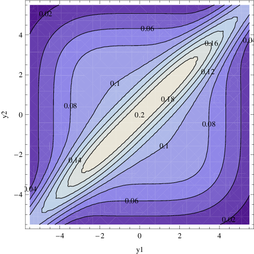
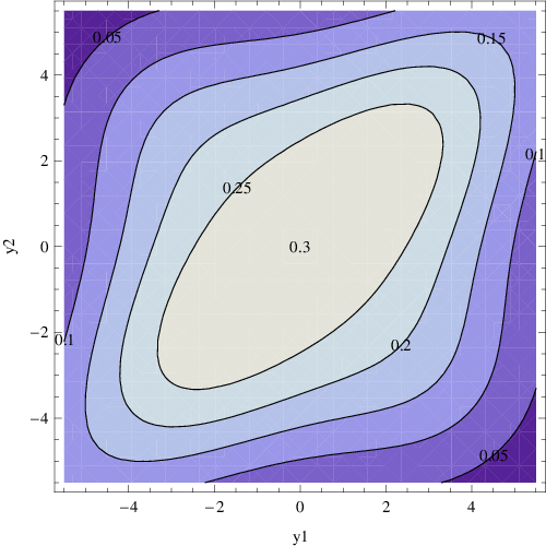
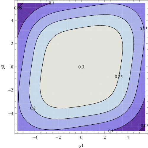
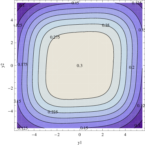
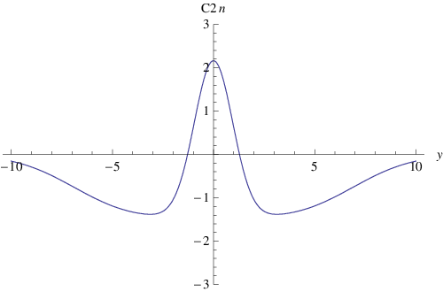
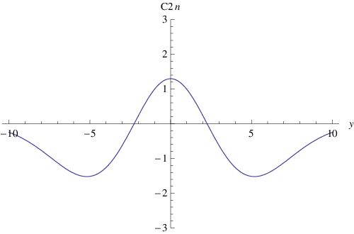
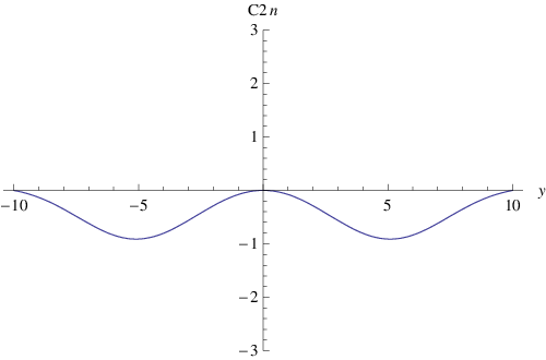
In Fig.3 we show for illustrative purposes several 2-dimensional plots of setting different rapidity correlation lengths: from (corresponding to 1212 12 The FWHM of the Gaussian is then about 2 rapidity units. in p-p collisions [19]), up to a very large value, (corresponding to production of extremely massive hidden (un)particles). All these plots are illustrative examples rather than actual predictions.
On the other hand, in a conventional multiparticle production process the maximum value of the correlation function is expected to decrease as higher multiplicities cuts are applied on events, as proven by experimental results [101]. An opposite behaviour would hint at NP on account of the enhancing LRC term in Eq.(37) due to the HS contribution. Moreover, let us note the square-shape of the contour-lines when the correlation length becomes comparable to the plateau length in the one-particle spectrum, an early warning about possible NP effects.
5.4 Semi-inclusive analysis
In order to remove as much as possible those non-dynamical fluctuations caused by unitarity, a semi-inclusive analysis of multiparticle production can be carried out, thereby providing an insight into the dynamical 1313 13 Let us point out, however, that the enhanced strength of LRC due to unitarity ought to be attributed ultimately to the underlying dynamics of a HS. correlations of particles emitted by clusters/clans (see, for example, [120, 119]) or even larger structures like Great-Clans as advocated in this paper.
The semi-inclusive 2-particle correlation function can be written as [119, 98]
| (44) |
where we have defined the single and double rapidity semi-inclusive densities of charged particles at fixed (charged) multiplicity in p-p collisions.
The above definition leads to the following normalizations:
| (45) |
Notice that these conditions force to be mostly negative.
In order to estimate the impact of a foreseen longer correlation length on , use will be made of the simple parametrization [119, 98]:
| (46) |
Motivated by Eq.(26), we tentatively set , while is tuned in order to satisfy the normalization (45). For definiteness we have chosen ; this choice is motivated by the reasonable expectation that a HS should rather manifest in high-multiplicity events. Notice that our actual claim is not providing predictions for , but an educated guess of the relative variation of the plotted curve as the correlation length varies.
In Fig.4 the semi-inclusive correlation function is plotted versus , for different values of the Gaussian parameter (and ). A narrow spike around generally stands up over a broad negative pedestal for SRC. Notice that longer correlations would show up in the plot by smoothing the curve which may become completely negative along the rapidity interval.
6 Forward-Backward correlations in a three-step scenario
Correlations between the charged-particle multiplicity in one hemisphere versus that of the other have been extensively studied in a wide range of center-of-mass energies, from bubble chamber experiments to LEP and Tevatron (see [33, 34] and references therein) for different beams and targets, in particular to understand the dynamics of dense matter in heavy-ion collisions [121, 122].
Following a parallel development, let us introduce in our analysis the well-known Forward-Backward (F-B) correlation parameter , defined as
| (47) |
where represents the multiplicity of the forward (backward) hemisphere, respectively, and is the corresponding variance, i.e.
| (48) |
Assuming no correlation between the forward and backward hemispheres, can be written as [102]
| (49) |
where the short-range part of should give no contribution in the numerator integral. Often a gap on the central region is excluded from the above intervals of integration to focus particularly on LRC; we will not consider this possibility in our study.
Moreover, a simple expression for can be obtained in a 2-step scenario, for the symmetrical situation corresponding to p-p collisions at the LHC, when ; one gets
| (50) |
where denotes the variance of the number of particles in single cluster decays 1414 14 Totally equivalent expressions involving heavy-ion collisions can be found, e.g., in [124, 123]..
The parameter introduced above is defined through
| (51) |
where and denote here the mean number and variance of clusters in each hemisphere.
The formula on the left side of Eq.(50) corresponds to a Poisson distribution for local particle emission from clusters (disregarding any hemisphere dependence) since then . Let us note that an expression similar to (50) is obtained according to the Color-Glass-Condensate approach [70] where LRC are in fact expected.
In a 3-step scenario, however, the above formula for is modified becoming
| (52) |
For and the expression for in Eq.(51) is recovered identifying and . Let us also note that Eqs.(51,52) can be put in correspondence with Eqs. (38,39).
Let us stress that, for Poissonian distributions and not too large (i.e. ), Eqs.(51,52) imply that is smaller than . We therefore suggest that a possible discrepancy found in the measurement of , together with other related observables from F-B correlations, in p-p collisions at the LHC (see e.g. [125] for predictions within the clan picture) could also shed light on a hidden (un)particle contribution to the parton cascade.
F-B correlations have been currently studied for different rapidity windows versus the gap size separating them. It is striking that in h-h collisions LRC effects persist up to a gap size of about 6 rapidity units [33]. Let us remark that very massive states at the onset of the cascade would imply stronger and even longer distance correlation effects, leading to larger cluster structures in rapidity space, thereby motivating the Great-Clan concept advocated in this work.
On the other hand, as mentioned in section 2.6, LRC stemming from Glasma formation related to the ridge” phenomenon discovered at RHIC [74] are actually not seen in p-p collisions, appearing to be unique to nucleus-nucleus collisions (since in the former case correlations are not collimated in azimuthal angle). Moreover, a growth of the LRC is predicted with the centrality of the collision in heavy-ion collisions. In any event, if very long-distance correlations were found in p-p inelastic collisions at the LHC, a dedicated study should be certainly carried out, comparing the results with RHIC and ALICE data, looking for distinctive features in order to reveal its true origin, either from a HS, from Glasma formation, or both.
7 Intermittency and fractal structure of the cascade
Fluctuations in small phase space regions (intermittency) have been commonly described by the scaled moments , where the rapidity interval under study is split into bins of equal size , as already commented in section 4.3. Moreover, the fractality nature of multiparticle hadroproduction (similar to a Cantor dust) is deeply connected with intermittent behaviour exhibiting a power-law dependence of the multiplicity moments with the cell size, as we shall later see.
For a smooth” (rapidity) distribution, not showing any fluctuation but the statistical ones, the moments should become independent of in the limit . On the contrary, if self-similar dynamical fluctuations exist, should obey a power-law increase at small , i.e.
| (53) |
For practical reasons, this power-law scaling (commonly called -scaling) is expressed as
| (54) |
where are called intermittency exponents’’. The above power-law dependence of the scaled factorial multiplicity moments 1515 15 Sometimes in the literature, intermittency may refer to any increase of the factorial moments with decreasing phase space intervals without need of a scaling behaviour as shown in Eq.(53). The extended version just indicates positive correlations in rapidity which increase at smaller bins. However, let us stress the relevance of the original proposal of intermittency connected with fractality through statistical self-similarity along the full cascade process. on the bin size is, in fact, a signature of self-similarity in the fluctuation pattern of the particle multiplicity [126].
In reality, particle correlations among emitted particles and intermittency could (should) also be studied using the normalized factorial cumulants (see footnote ) instead of , as for example carried out by OPAL in the study of hadronic decays [52, 108]. Once experimental data become available from LHC experiments, the analysis of factorial cumulants will become compulsory in p-p inelastic events. Meanwhile, we restrict our study to the power-law behaviour given by (53).


7.1 Numerical estimates of normalized factorial moments
Our main concern in this section is to investigate about the multi- or mono-fractal nature of the showering process in a two-step scenario versus three-step scenario. We shall study the intermittency foreseen for multiplicity distributions in p-p collisions. Our goal is by no means giving predictions”, rather we want to assess the sensitivity of some fractality estimators to a hypothetical non-standard step in the hadroproduction cascade, once experimental data from LHC become available. To this aim, we will rely upon the estimates of from Eqs.(32) and (40), and on the scaling relations of Eq.(17) for the moments of higher rank.
Let us first compute by making the assumption that and thereby display the exponential form of Eqs.(34,11). Let us remark that whenever we consider a 3-step scenario, we extend the concept of cluster up to a Great-Clan, i.e. quite more final-state particles are correlated than in a single cluster assuming that the effective correlation length becomes larger.
Upon integration of Eq.(33) one gets
| (55) |
where , and
| (56) |
Note that for small (i.e. ), and for large (i.e. ).
In our toy model, the LRC term was assumed to be a constant, so the resulting (multi)fractality derives from the single cluster decay via the behaviour of as a function of or . The limit when is negligible as compared to such a constant LRC term implies in fact nonfractality.
In Fig.5 we show a set of double logarithmic plots for several normalized factorial moments of the multiplicity distribution, and (from down to up), versus the (pseudo)rapidity binning . The curves have been naively calculated by assuming Poisson-like distributions for all particle sources. Dashed (solid) lines refer to expectations from a conventional two-step (three-step) cascade employing Eqs.(32) and (40) with different assignments for the average numbers of unparticles and clusters. Besides we assumed and for the 2- and 3-step cascades, respectively.
The examples shown in Fig.5 correspond to:
- a)
, and ,
- b)
, and
- c)
, and .
In reality, the bin size dependence of does not follow a power-like law in the whole rapidity interval, but can be fitted separately by power laws for large/small bins. Hereafter we restrict our attention to the more or less linear region between and before the levelling-off.
From inspection of these plots we can conclude that:
- •
The height of all curves may vary significantly when passing from one scenario to another. Although an increase or decrease of the asymptotic values (i.e. at large ) may result depending on the assumptions for , and , higher curves generally stem from for the 3-step chain, provided that , as already pointed out in section 5.2.1.
- •
The slopes differ appreciably when comparing the two-step against the tree-step cascade, especially for higher values. This fact could be anticipated because of the expected larger constant contribution to the correlation function in the latter case. As we shall see, the multifractality revealed by the -dependence of weakens accordingly.
The intermittent behaviour observed by many experiments (see e.g.[34, 106, 107, 108, 127, 128, 129, 110]) in the analysis of factorial moments of spectra of emitted secondaries indicate the existence of some multifractal structure of the production process. We will address this issue in the following section, using the results” from our toy model shown in Fig.5.
7.2 Fractality
As mentioned above, hadronization exhibits a self-similarity pattern and therefore a multifractal structure: the pictorial description of jets within jets, within jets is commonly employed to illustrate this behaviour. In this regard, the Lund group [130] presented a suggestive interpretation of the cascade based on a colour dipole picture by means of a multi-faceted surface due to the consecutive emission of many gluons. Because of its iterative nature, the process generates a Koch-type fractal curve at the base-line, whose length is proportional to the particle multiplicity. This curve becomes longer when analized with higher resolution: it is indeed a fractal curve characterized by the fractal dimension , where stands for the QCD anomalous dimension.
Accordingly, the multiplicity of emitted particles in small phase space intervals should show intermittent features, with multifractal (Rényi) dimension for large . The multifractal dimension and the anomalous fractal dimension are related through: [131]; in turn , which is a measure for the deviation of from an integer, can be related to the intermittency coefficient as:[132, 133]
| (57) |
It has been widely argued in the literature since Ref.[134] that if QGP is created in hadronic collisions, a phase transition to hadron matter must take place. If such a transition is close to second-order the outgoing hadron system should show intermittency with weakly depending on in contrast to an approximate linear dependence when a cascade process occurs.


Let us remark that for a second-order phase transition from plasma to hadrons the correlation length should be larger than the size of the largest system produced. This indeed resembles the claim of this paper when a new state of matter is assumed at the onset of the showering.
In Fig.6 we show the behaviour of for obtained from our toy analysis based on the (pseudo)rapidity binning. One can quickly see that the -dependence of weakens in the three-step scenario. This is in fact a general feature for almost every reasonable parameter combination in our study as could be expected as a consequence of long-range correlations (both from , and associated to a larger ) yielding stronger contributions to the moments. This conclusion agrees with the experimental finding that the anomalous dimension generally decreases for a growing complexity of the process (e.g. from muon-proton, p-p, to p-A and A-A interactions), theoretically accounted for in [132].
7.3 Ratios of intermittency exponents
Another interesting feature closely related to the above discussion is the power scaling between and , i.e.
| (58) |
commonly known as -scaling, obviously implying
| (59) |
where the coefficient can be expressed as
| (60) |
Notice that the validity of -scaling as shown in Eq.(53) guarantees the validity of -scaling, but Eq.(58) may be valid even if Eq.(53) is not.
In Fig.6 (middle), the corresponding lines derived from our toy model are drawn for . Monofractality () of course implies .
As mentioned previously, one could (should) consider the factorial cumulant as a function of in a more realistic study, or when using experimental data. In our case, no additional information would be really added following up from such study due to the simplicity of our framework.
| Scenario | |||||
|---|---|---|---|---|---|
| 2-step | |||||
| 3-step |
7.3.1 Lévy stable law description
Brax and Peschanski [135] proposed a better approximation than Eq.(60) using a Lévy stable law description of multiparticle production. Hence instead of Eq(60) the -dependence of is given by:
| (61) |
where is the Lévy index (also known as the degree of multifractality) which allows an estimation of the cascading rate; should be in principle restricted to the interval (region of stability). Some violations of this limit have been found in the analysis of experimental data in h-h collisions [33, 34], though can be adequately reinterpreted by invoking high anisotropy of phase space in multiparticle production [136].
The introduction of the parameter helps classifying intermittency patterns due to different kinds of phase transitions, either thermal (e.g. quark-gluon plasma), or non-thermal (cascading process).
Two extreme cases can be distinguished:
- •
: yielding , i.e. , corresponding to a self-similar branching process.
- •
: yielding , i.e. , the system displays a monofractal behaviour.
Whereas cascade models show a multifractal structure, a hadronic system undergoing a second-order transition should lead to intermittency associated to a monofractal structure. It is well-known that the experimental measurement of this coefficient in relativistic heavy-ion collisions should be useful in detecting the formation of QGP [137].
Motivated by the above remarks, we have studied using our toy model the -scaling in p-p inelastic collisions under the hypothesis of an extra stage from a HS. In Table 1 we present the values obtained for corresponding to both scenarios, providing two quite different values for the parameter: obtained for a conventional fragmentation chain, versus once a new state of matter has been added into the cascade. Our results are consistent with the interpretation that the production process approaches monofractality (or merely a loss of fractality as all values become smaller as can be seen from Fig.6) when a HS modifies the onset of the parton cascade. Note that unparticle stuff in particular could display itself a fractal nature acting as a fluctuating mass source 1616 16 A fractal structure of the source in space-time is discussed in [138, 139] of (clusters of) particles in the hadronization chain, on account of its continous mass spectrum.
Let us remark however that a full exploration of the fractal properties of multiparticle production actually requires a 3-dimensional analysis once experimental data become available at the LHC.
| 2 | 0.72 | 1.18 | 2 | 2 | 4 | 0.60 | 1.15 |
| 4 | 1.10 | 1.30 | 1 | 4 | 4 | 0.43 | 1.10 |
| 6 | 1.29 | 1.37 | 3 | 4 | 12 | 0.98 | 1.26 |
| 8 | 1.46 | 1.42 | 2 | 4 | 8 | 0.72 | 1.18 |
| 10 | 1.50 | 1.45 | 1 | 10 | 10 | 0.50 | 1.12 |
| 18 | 1.69 | 1.52 | 3 | 6 | 18 | 1.01 | 1.27 |
| 24 | 1.75 | 1.55 | 2 | 10 | 20 | 0.85 | 1.22 |
7.3.2 Ginzburg-Landau description
The Ginzburg-Landau (GL) theory [140] has been applied to a wide variety of phase state transition phenomena, from superconductivity to quark-gluon matter [103]. Here we seek a (hopefully fruitful) analogy between our approach to the quest for a HS in p-p inelastic collisions, and a GL description of the deconfining phase transition from QGP to hadronic matter [9, 141].
Instead of the law expressed in Eq.(61), is parametrized now as
| (62) |
where characterizes the critical phase transition, ordinarily implying monofractality. The universal” exponent was computed analytically in [9] for a second order transition, finding .
Once again, we perform a comparison between the expected value according to a standard cascade versus the value obtained under the assumption of an extra stage associated to a HS, based on our toy model. In Fig.6 (right) we show the result of the power-fit Eq.(62) of as a function of obtained from data” collected in Table for in both scenarios. In this particular example, we find and , for the two- and three-step cascade, respectively.
In addition, Table 2 shows several more couples of and exponents, to be used as quantitative estimators of the fractal character of the cascade obtained for different parameter combinations. Let us stress again that our goal is not making predicitions on and , but estimating the relative variation in both scenarios. One can indeed conclude that both and values turn out to be systematically smaller in a 3-step cascade than in a 2-step scenario, remarkably even when . Notice, however, the increase of and with a growing , i.e. the average number of (un)particles from a HS involved in the cascade. Hopefully, the foreseen differences will allow to distinguish experimentally between the two scenarios using p-p data to be collected soon at the LHC [4].
7.3.3 Discussion
Since multifractality is generally viewed as a manifestation of a self-similar random cascade (i.e. a non-thermal process), it may seem striking that adding a new step to the parton avalanche would imply the opposite effect, i.e. getting closer to monofractality usually associated with (second-order) thermal transitions in heavy-ion collisions. This apparently paradoxical result could be seen, however, in accordance with the existence of a larger correlation length in a three-step scenario with heavy hadronic objects initiating the hadronization chain. The new state of matter would, in an effective way, play an analagous role to that expected for QGP in central heavy-ion collisions.
8 Summary and prospects
In hadron-induced reactions, multiparticle production is generally described as proceeding through a two-step process. First the interaction between the colliding constituents (active partons) gives rise to strings/clusters/clans/fireballs, subsequently decaying through a QCD cascade and soft hadronization into final-state SM particles. Of course, hadroproduction is actually a much more complex process because of extra event activity caused by parton remnants, initial and final-state radiation, etc.
New physics associated to higher mass scales is generally expected to show up in high- events. In this work, however, we have focused on rather diffuse soft signals in p-p inelastic interactions, likely tagged by hard decay products. We argued that a non-standard state of matter from a HS (e.g. unparticle stuff) would give rise to a three-step cascade in hadron collisions, altering observables related to rapidity particle correlations which can be determined at the LHC to a large accuracy.
On the one hand, two-particle (or higher) rapidity correlation functions are sensitive to a longer correlation length caused by either fluctuations in the number of particle sources, or (very) massive intermediate state decays. Expectedly both and functions should develop a plateau in a two-dimensional plot along the diagonal of similar length as the single-particle spectrum, furnishing a (or scale) to determine dynamical correlations, e.g., along the perpendicular diagonal . Naively, a square-shape of contour-lines at mid-rapidities and an increase of with event multiplicity might hint at NP. Moreover, since CGC/Glasma also predicts LRC, a comparative study between A-A collisions and p-p collisions should be performed to find out distinctive signatures of a HS from extended rapidity sources expected in QCD.
By fixing the multiplicity of events, those LRC due to unitarity constraints should be largely suppressed as the different sources (at any stage) are not yet allowed to fluctuate freely. We have checked that a semi-inclusive analysis could therefore be useful to determine a correlation length likely longer than expected in a conventional parton showering, due to the large size of clans (dubbed Great-Clans) stemming from a HS. We also performed a study of forward-backward correlations concluding again that a HS could modify the correlation parameter usually defined for such analyses.
On the other hand, the afore-mentioned three-step scenario would imply a sizable modification of the power-law dependence (intermittency) of the normalized factorial moments versus the phase space (pseudorapidity) binning. Determining the multifractality nature of multiparticle production could be useful to assess the hypothetical contribution from a HS. Our main conclusion is that those cascades initiated by very massive hidden (un)particles should become less multifractal (= more monofractal or merely less fractal) than in conventional events, basically because of a larger correlation length, leading to a suggestive (though formal) resemblance with a second-order phase transition from QGP to deconfined hadrons in heavy-ion collisions, in spite of very different underlying physical processes.
We thereby have worked out a detailed exercise” on - and -scaling of factorial moments, applying both Lévy law and Ginzburg-Landau descriptions, commonly used in the search for QGP. Several reference values for the and exponents (related to the cascade character of the production process) were obtained as illustrative examples (not actual predictions). We concluded that both estimators should be smaller in a 3-step cascade than in a 2-step process, hopefully providing a quantitative way of assessing the presence of a HS in the cascade once experimental data are employed.
Other techniques to obtain relic information carried out by final-state particles about their (grand) parent state, not addressed in this paper, should be considered however in a future extension of this work: azimuthal correlations, rapidity gaps, etc. Besides, note that correlations should be stronger in multi-dimensional phase-space [142] than in a lower dimensional projection like rapidity space 1717 17 This feature is pictorially described in [106] by comparing the (rather continuous) two-dimensional shadow of a tree, and the self-similar branching of this tree in three-dimensional space..
Proposal
Generally speaking, the search strategy for new phenomena consists in distinguishing the characteristic signal from the SM background. Direct signals (e.g. based on jets or missing energy/) from a new state of non-standard matter (i.e. from a hidden sector) can be difficult to observe, and/or discriminate among different possibilities yielding similar phenomenology. Our proposal can thus be seen as a way of optimizing all the potential information to be obtained from LHC, Tevatron and RHIC experiments: an example of sinergy.
To this aim, looking back at the impressive work already done in the analysis of high-energy hadron-hadron collisions, we have put forward a complementary inclusive analysis of multiparticle dynamics in inelastic p-p collisions based on (pseudo)rapidity correlations among the emitted hadrons. In addition, correlations between hadrons and photons should also be of great interest, especially in certain HS models predicting a large rate of soft photon radiation in events.
Selection (off-line) cuts should be applied to a statistically significant sample of MBE’s based on criteria like: high multiplicity and sphericity, jet activity (not necessarily large- jets) and, probably, model-dependent criteria such as requiring heavy flavour, multiple leptons and/or photons in the final state. Those events not passing the cuts should play the role of the null hypothesis in a hypothesis test [143] on the existence of a HS manifesting in semi-hard physics.
Needless to say, a much more complete study including a realistic modeling of hadroproduction and simulation of detector effects is required to decide about the usefulness of this proposal.
Acknowledgments
I gratefully acknowledge Carlos Garcia-Canal, Emilio Higon, Vicent Martinez,
Vasiliki Mitsou, Lluis Oliver, Carlos Pajares,
Joannis Papavassiliou and Edward Sarkisyan-Grinbaum for many useful
comments. I also thank MICINN and Generalitat Valenciana for financial support
under research grants FPA2005-01678, FPA2008-02878 and GVPRE/2008/003.
Since this paper refers to a lot of background material and references,
apologies for possible oversights totally unintended.
References
- [1] M. L. Mangano, arXiv:0802.0026 [hep-ph]; M. L. Mangano, arXiv:0809.1567 [hep-ph].
- [2] R. Harnik and T. Wizansky, arXiv:0810.3948 [hep-ph].
- [3] A. Giovannini and R. Ugoccioni, Phys. Rev. D 68 (2003) 034009 [arXiv:hep-ph/0304128].
- [4] G. Aad et al. [ATLAS Collaboration], JINST 3 (2008) S08003; R. Adolphi et al. [CMS Collaboration], JINST 3 (2008) S08004; A. A. Alves et al. [LHCb Collaboration], JINST 3 (2008) S08005.
- [5] K. Aamodt et al. [ALICE Collaboration], JINST 3 (2008) S08002.
- [6] J. D. Wells, arXiv:0803.1243 [hep-ph].
- [7] B. J. T. Jones, V. J. Martinez, E. Saar and V. Trimble, Rev. Mod. Phys. 76 (2005) 1211 [arXiv:astro-ph/0406086].
- [8] M. J. Tannenbaum, J. Phys. Conf. Ser. 27 (2005) 1 [arXiv:nucl-ex/0507020].
- [9] R. C. Hwa and M. T. Nazirov, Phys. Rev. Lett. 69 (1992) 741; R. C. Hwa and J. c. Pan, Phys. Lett. B 297 (1992) 35; R. C. Hwa, Phys. Rev. D 47 (1993) 2773.
- [10] I. M. Dremin and C. Quigg, Science 199, 937 (1978) [Usp. Fiz. Nauk 124, 535 (1978)].
- [11] E. Fermi, Prog. Theor. Phys. 5 (1950) 570.
- [12] K.G.Wilson, Proc. Fourteen Scottish Universities Summer School in Physics (1973), edited by R.L. Crawford and R. Jennings (Academic Press, New York, 1974).
- [13] S. Z. Belenkij and L. D. Landau, Nuovo Cim. Suppl. 3S10 (1956) 15 [Usp. Fiz. Nauk 56 (1955) 309]; L. D. Landau, Izv. Akad. Nauk Ser. Fiz. 17 (1953) 51.
- [14] R. Hagedorn and J. Ranft, Nuovo Cim. Suppl. 6 (1968) 169.
- [15] S. Fubini and G. Veneziano, Nuovo. Cim. A 64 (1969) 811.
- [16] N. Cabibbo and G. Parisi, Phys. Lett. B59 (1975) 67.
- [17] W. R. Frazer et al., Rev. Mod. Phys. 44 (1972) 284.
- [18] J. L. Meunier and G. Plaut, Nucl. Phys. B 87 (1975) 74; E. L. Berger and G. C. Fox, Phys. Lett. B 47 (1973) 162.
- [19] B. Alver et al. [PHOBOS Collaboration], Phys. Rev. C 75 (2007) 054913 [arXiv:0704.0966 [nucl-ex]].
- [20] R. E. Ansorge et al. [UA5 Collaboration], Z. Phys. C 37 (1988) 191.
- [21] B. Andersson, G. Gustafson, M. Ringner and P. J. Sutton, Eur. Phys. J. C 7 (1999) 251 [arXiv:hep-ph/9808436].
- [22] F. H. Liu, Y. Yuan and M. Y. Duan, Nucl. Phys. A 801 (2008) 154.
- [23] F. H. Liu, Nucl. Phys. A 810 (2008) 159.
- [24] J. Benecke, T. T. Chou, C. N. Yang and E. Yen, Phys. Rev. 188, 2159 (1969).
- [25] I. Otterlund et al., Nucl. Phys. B 142 (1978) 445.
- [26] W. Busza, J. Phys. G 35 (2008) 044040 [arXiv:0710.2293 [nucl-ex]].
- [27] E. K. G. Sarkisyan and A. S. Sakharov, AIP Conf. Proc. 828 (2006) 35 [arXiv:hep-ph/0510191]; E. K. G. Sarkisyan and A. S. Sakharov, arXiv:hep-ph/0410324.
- [28] A. Akindinov et al., Eur. Phys. J. C 50 (2007) 341 [arXiv:0709.1664 [hep-ph]].
- [29] A. Moraes, C. Buttar and I. Dawson, Eur. Phys. J. C 50, 435 (2007).
- [30] M. Mitrovski, T. Schuster, G. Graef, H. Petersen and M. Bleicher, arXiv:0812.2041 [hep-ph].
- [31] A. Bialas and M. Jezabek, Phys. Lett. B 590 (2004) 233 [arXiv:hep-ph/0403254].
- [32] A. Capella, U. Sukhatme, C. I. Tan and J. Tran Thanh Van, Phys. Rept. 236 (1994) 225.
- [33] W. Kittel, Acta Phys. Polon. B 35 (2004) 2817.
- [34] W. Kittel and E. A. De Wolf, “Soft Multihadron Dynamics,” World Scientific 2005
- [35] Z. Koba, H. B. Nielsen and P. Olesen, Nucl. Phys. B 40 (1972) 317.
- [36] T. Kanki, K. Kinoshita, H. Sumiyoshi and F. Takagi, Prog. Theor. Phys. Suppl. 97B (1989) 1.
- [37] A. O. Bouzas, L. N. Epele, H. Fanchiotti and C. A. Garcia Canal, Z. Phys. C 56 (1992) 107.
- [38] S. Hegyi, Phys. Lett. B 467 (1999) 126; S. Hegyi, Phys. Lett. B 466 (1999) 380.
- [39] A. M. Polyakov, JETP Lett. 12 (1970) 381 [Pisma Zh. Eksp. Teor. Fiz. 12 (1970) 538].
- [40] I. M. Dremin and J. W. Gary, Phys. Rept. 349 (2001) 301 [arXiv:hep-ph/0004215].
- [41] I. M. Dremin and V. A. Nechitailo, Phys. Rev. D 70, 034005 (2004) [arXiv:hep-ph/0402286].
- [42] E. K. G. Sarkisyan, Phys. Lett. B 477, 1 (2000) [arXiv:hep-ph/0001262].
- [43] A. Giovannini and L. Van Hove, Z. Phys. C 30 (1986) 391; A. Giovannini and L. Van Hove, Acta Phys. Polon. B 19 (1988) 495.
- [44] A. Giovannini and R. Ugoccioni, Int. J. Mod. Phys. A 20 (2005) 3897 [arXiv:hep-ph/0405251].
- [45] M. Brambilla, A. Giovannini and R. Ugoccioni, arXiv:hep-ph/0605269.
- [46] A. Giovannini, S. Lupia and R. Ugoccioni, Phys. Rev. D 65 (2002) 094028 [arXiv:hep-ph/0203205].
- [47] A. B. Kaidalov and K. A. Ter-Martirosyan, Sov. J. Nucl. Phys. 40 (1984) 135 [Yad. Fiz. 40 (1984) 211].
- [48] B. Andersson, G. Gustafson, G. Ingelman and T. Sjostrand, Phys. Rept. 97 (1983) 31.
- [49] B. B. Back et al. [PHOBOS Collaboration], arXiv:nucl-ex/0301017; B. B. Back et al. [PHOBOS Collaboration], Phys. Rev. C 74 (2006) 021902; S. Manly et al. [PHOBOS Collaboration], Nucl. Phys. A 774 (2006) 523 [arXiv:nucl-ex/0510031].
- [50] L. Cunqueiro, J. Dias de Deus and C. Pajares, arXiv:0806.0523 [hep-ph].
- [51] I. M. Dremin, Phys. Atom. Nucl. 68 (2005) 758 [Yad. Fiz. 68 (2005) 790] [arXiv:hep-ph/0404202].
- [52] G. Abbiendi et al. [OPAL Collaboration], Phys. Lett. B 638 (2006) 30 [arXiv:hep-ex/0604003].
- [53] T. Sjostrand and M. van Zijl, Phys. Rev. D 36 (1987) 2019.
- [54] T. Sjostrand, arXiv:0809.0303 [hep-ph].
- [55] B. Andersson, The Lund Model (Cambridge University Press, 1998).
- [56] T. Sjostrand, S. Mrenna and P. Skands, Comput. Phys. Commun. 178, 852 (2008) [arXiv:0710.3820 [hep-ph]].
- [57] H. Muller, Eur. Phys. J. C 18 (2001) 563 [arXiv:hep-ph/0011350].
- [58] G. H. Arakelyan, C. Merino, C. Pajares and Yu. M. Shabelski, Eur. Phys. J. C 54 (2008) 577 [arXiv:0709.3174 [hep-ph]].
- [59] K. Adcox et al. [PHENIX Collaboration], Nucl. Phys. A 757 (2005) 184 [arXiv:nucl-ex/0410003].
- [60] T. Matsui and H. Satz, Phys. Lett. B 178 (1986) 416.
- [61] N. Brambilla et al. [Quarkonium Working Group], arXiv:hep-ph/0412158.
- [62] I. Arsene et al. [BRAHMS Collaboration], Nucl. Phys. A 757 (2005) 1 [arXiv:nucl-ex/0410020].
- [63] N. S. Amelin, N. Armesto, M. A. Braun, E. G. Ferreiro and C. Pajares, Phys. Rev. Lett. 73 (1994) 2813.
- [64] N. G. Antoniou, F. K. Diakonos, C. N. Ktorides and M. Lahanas, Phys. Lett. B 432 (1998) 8.
- [65] Y. V. Kovchegov, E. Levin and L. D. McLerran, Phys. Rev. C 63 (2001) 024903 [arXiv:hep-ph/9912367].
- [66] S. A. Voloshin, J. Phys. Conf. Ser. 50 (2006) 111 [arXiv:nucl-ex/0505003].
- [67] J. Adams et al. [STAR Collaboration], Phys. Rev. Lett. 97 (2006) 162301 [arXiv:nucl-ex/0604018].
- [68] F. Noferini, Eur. Phys. J. C 52 (2007) 247.
- [69] L. D. McLerran and R. Venugopalan, Phys. Rev. D 49 (1994) 3352 [arXiv:hep-ph/9311205]; L. D. McLerran and R. Venugopalan, Phys. Rev. D 49 (1994) 2233 [arXiv:hep-ph/9309289].
- [70] N. Armesto, L. McLerran and C. Pajares, Nucl. Phys. A 781 (2007) 201.
- [71] Y. V. Kovchegov, arXiv:0811.2438 [hep-ph].
- [72] L. McLerran, arXiv:0812.4989 [hep-ph].
- [73] B. K. Srivastava, R. P. Scharenberg and T. J. Tarnowsky, arXiv:nucl-ex/0702040; B. K. Srivastava [STAR Collaboration], Int. J. Mod. Phys. E 16 (2008) 3371 [arXiv:nucl-ex/0702054].
- [74] A. Dumitru, F. Gelis, L. McLerran and R. Venugopalan, Nucl. Phys. A 810 (2008) 91 [arXiv:0804.3858 [hep-ph]].
- [75] R. Field [CDF Collaboration], AIP Conf. Proc. 928 (2007) 91.
- [76] P. Z. Skands, FERMILAB-CONF-07-706-T.
- [77] H. Georgi, Phys. Rev. Lett. 98 (2007) 221601 [arXiv:hep-ph/0703260]; H. Georgi, Phys. Lett. B 650 (2007) 275 [arXiv:0704.2457 [hep-ph]].
- [78] H. Nikolic, Mod. Phys. Lett. A 23 (2008) 2645 [arXiv:0801.4471 [hep-ph]].
- [79] T. Kikuchi and N. Okada, Phys. Lett. B 661, 360 (2008) [arXiv:0707.0893 [hep-ph]].
- [80] F. Sannino and R. Zwicky, arXiv:0810.2686 [hep-ph].
- [81] P. J. Fox, A. Rajaraman and Y. Shirman, Phys. Rev. D 76 (2007) 075004 [arXiv:0705.3092 [hep-ph]]; A. Delgado, J. R. Espinosa and M. Quiros, JHEP 0710 (2007) 094 [arXiv:0707.4309 [hep-ph]];
- [82] T. Kikuchi and N. Okada, Phys. Lett. B 665, 186 (2008) [arXiv:0711.1506 [hep-ph]].
- [83] H. Davoudiasl, Phys. Rev. Lett. 99 (2007) 141301 [arXiv:0705.3636 [hep-ph]]; S. L. Chen, X. G. He, X. P. Hu and Y. Liao, arXiv:0710.5129 [hep-ph]; B. Grzadkowski and J. Wudka, arXiv:0809.0977 [hep-ph].
- [84] X. G. He and L. Tsai, JHEP 0806 (2008) 074 [arXiv:0805.3020 [hep-ph]]; M. Luo and G. Zhu, Phys. Lett. B 659 (2008) 341 [arXiv:0704.3532 [hep-ph]].
- [85] M. Neubert, Phys. Lett. B 660 (2008) 592 [arXiv:0708.0036 [hep-ph]].
- [86] J. L. Feng, A. Rajaraman and H. Tu, Phys. Rev. D 77 (2008) 075007 [arXiv:0801.1534 [hep-ph]]
- [87] K. Cheung, W. Y. Keung and T. C. Yuan, arXiv:0809.0995 [hep-ph].
- [88] A. Rajaraman, arXiv:0806.1533 [hep-ph].
- [89] A. Delgado, J. R. Espinosa, J. M. No and M. Quiros, arXiv:0812.1170 [hep-ph].
- [90] M. J. Strassler and K. M. Zurek, Phys. Lett. B 651, 374 (2007) [arXiv:hep-ph/0604261]; M. J. Strassler, arXiv:0801.0629 [hep-ph]; M. J. Strassler, arXiv:0806.2385 [hep-ph].
- [91] T. Han, Z. Si, K. M. Zurek and M. J. Strassler, JHEP 0807 (2008) 008 [arXiv:0712.2041 [hep-ph]]; M. J. Strassler, arXiv:hep-ph/0607160.
- [92] B. Patt and F. Wilczek, arXiv:hep-ph/0605188.
- [93] S. Chang, R. Dermisek, J. F. Gunion and N. Weiner, arXiv:0801.4554 [hep-ph].
- [94] F. Domingo, U. Ellwanger, E. Fullana, C. Hugonie and M. A. Sanchis-Lozano, arXiv:0810.4736 [hep-ph].
- [95] A. Belyaev, R. Foadi, M. T. Frandsen, M. Jarvinen, A. Pukhov and F. Sannino, arXiv:0809.0793 [hep-ph].
- [96] J. Kang and M. A. Luty, arXiv:0805.4642 [hep-ph].
- [97] S. B. Giddings and S. D. Thomas, Phys. Rev. D 65 (2002) 056010 [arXiv:hep-ph/0106219]; S. Dimopoulos and G. L. Landsberg, Phys. Rev. Lett. 87 (2001) 161602 [arXiv:hep-ph/0106295].
- [98] L. Foa, Phys. Rept. 22, 1 (1975); S. R. Amendolia et al., Phys. Lett. B 48, 359 (1974); R. Singer et al., Phys. Lett. B 49 (1974) 481
- [99] R. J. Porter and T. A. Trainor [STAR Collaboration], J. Phys. Conf. Ser. 27 (2005) 98 [arXiv:hep-ph/0506172].
- [100] L. Simic et al., Z. Phys. C 2 (1979) 291; J. M. Bolta, E. Higon and M. A. Sanchis, Nuovo Cim. A 59 (1980) 173; D. Ghosh, J. Roy, M. Basu, K. Sengupta, S. Naha, A. Bhattacharyya and T. G. Thakurta, Phys. Rev. D 26 (1982) 2983.
- [101] A. Breakstone et al. [ABCDHW Collaboration], Phys. Lett. B 114 (1982) 383.
- [102] A. Capella and A. Krzywicki, Phys. Rev. D 18 (1978) 4120.
- [103] T. Abbott et al. [E-802 Collaboration], Phys. Rev. C 52 (1995) 2663; S. S. Adler et al. [PHENIX Collaboration], Phys. Rev. C 76 (2007) 034903 [arXiv:0704.2894 [nucl-ex]].
- [104] T. Csorgo, S. Hegyi, T. Novak and W. A. Zajc, Acta Phys. Polon. B 36 (2005) 329 [arXiv:hep-ph/0412243].
- [105] I. V. Andreev, M. Biyajima, I. M. Dremin and N. Suzuki, Int. J. Mod. Phys. A 10 (1995) 3951 [arXiv:hep-ph/9501345].
- [106] E. A. De Wolf, I. M. Dremin and W. Kittel, Phys. Rept. 270 (1996) 1 [arXiv:hep-ph/9508325].
- [107] A. Capella, K. Fialkowski and A. Krzywicki, LPTHE-ORSAY-89-21, Conference on Multiparticle Dynamics, La Thuile, Italy, Mar 20-22, 1989.
- [108] G. Abbiendi et al. [OPAL Collaboration], Phys. Lett. B 523 (2001) 35 [arXiv:hep-ex/0110051]; G. Abbiendi et al. [OPAL Collaboration], Eur. Phys. J. C 11 (1999) 239 [arXiv:hep-ex/9902021].
- [109] A. M. Tawfik, arXiv:hep-ph/0012022.
- [110] J. S. Li, F. H. Liu and D. H. Zhang, Chin. Phys. Lett. 24 (2007) 2789; D. H. Zhang et al., Chin. Phys. i16 (2007) 2689; D. H. Zhang et al., Chin. Phys. 16 (2007) 2683 [Radiat. Meas. 43 (2008) S258].
- [111] I. M. Dremin, Mod. Phys. Lett. A 8 (1993) 2747.
- [112] L. L. Chau and D. W. Huang, Phys. Lett. B 283 (1992) 1.
- [113] A. Bialas and R. B. Peschanski, Nucl. Phys. B 273 (1986) 703; A. Bialas and R. B. Peschanski, Nucl. Phys. B 308 (1988) 857.
- [114] P. Carruthers and I. Sarcevic, Phys. Rev. Lett. 63, 1562 (1989) [Erratum-ibid. 63, 2612 (1989)].
- [115] W. Ochs and J. Wosiek, Phys. Lett. B 214 (1988) 617.
- [116] P. Carruthers and M. Duong-Van, LA-UR-83-2419.
- [117] S. Uhlig, I. Derado, R. Meinke and H. Preissner, Nucl. Phys. B 132 (1978) 15.
- [118] G. Alexander and E. Sarkisyan, Phys. Lett. B 487 (2000) 215 [arXiv:hep-ph/0005212]; G. Alexander and E. Sarkisyan, Nucl. Phys. Proc. Suppl. 92 (2001) 211 [arXiv:hep-ph/0008174].
- [119] E. L. Berger, Nucl. Phys. B 85 (1975) 61.
- [120] W. Bell et al. [CERN-Heidelberg-Lund Collaboration], Z. Phys. C 22 (1984) 109.
- [121] L. Cunqueiro, E. G. Ferreiro and C. Pajares, PoS C FRNC2006 (2006) 019 [arXiv:hep-ph/0611034]; J. Dias de Deus, C. Pajares and C. A. Salgado, Phys. Lett. B 407 (1997) 335 [arXiv:hep-ph/9702398].
- [122] N. Armesto et al., J. Phys. G 35 (2008) 054001 [arXiv:0711.0974 [hep-ph]]
- [123] P. Brogueira and J. Dias de Deus, Phys. Lett. B 653 (2007) 202 [arXiv:hep-ph/0611329].
- [124] P. Brogueira, J. Dias de Deus and J. G. Milhano, Phys. Rev. C 76 (2007) 064901
- [125] A. Giovannini and R. Ugoccioni, Phys. Rev. D 66 (2002) 034001 [arXiv:hep-ph/0205156].
- [126] I. M. Dremin, FERMILAB-PUB-89-071-T.
- [127] C. Albajar et al. [UA1 Collaboration], Z. Phys. C 56 (1992) 37.
- [128] E. K. Sarkisian, L. K. Gelovani, G. L. Gogiberidze and G. G. Taran, Phys. Lett. B 347 (1995) 439 [arXiv:hep-ph/9412336].
- [129] S. Ahmad and M. A. Ahmad, J. Phys. G 32 (2006) 1279.
- [130] P. Dahlqvist, B. Andersson and G. Gustafson, Nucl. Phys. B 328 (1989) 76; B. Andersson, G. Gustafson, A. Nilsson and C. Sjogren, Z. Phys. C 49 (1991) 79; G. Gustafson and A. Nilsson, Nucl. Phys. B 355 (1991) 106; G. Gustafson and A. Nilsson, Z. Phys. C 52 (1991) 533.
- [131] W. Ochs and J. Wosiek, Phys. Lett. B 305 (1993) 144.
- [132] P. Lipa and B. Buschbeck, Phys. Lett. B 223 (1989) 465.
- [133] R. C. Hwa, Phys. Rev. D 41 (1990) 1456.
- [134] A. Bialas and R. C. Hwa, Phys. Lett. B 253 (1991) 436.
- [135] P. Brax and R. B. Peschanski, Phys. Lett. B 253 (1991) 225.
- [136] Y. Zhang, L. S. Liu and Y. f. Wu, Z. Phys. C 71 (1996) 499.
- [137] A. M. Tawfik, arXiv:hep-ph/0104004; A. M. Tawfik and E. Ganssauge, Heavy Ion Phys. 12 (2000) 53 [arXiv:hep-ph/0012008].
- [138] A. Bialas, Acta Phys. Polon. B 23 (1992) 561.
- [139] O. V. Utyuzh, G. Wilk and Z. Wlodarczyk, Czech. J. Phys. 50S2 (2000) 132 [arXiv:hep-ph/9910355].
- [140] V. L. Ginzburg and L. D. Landau, Zh. Eksp. Teor. Fiz. 20 (1950) 1064.
- [141] Z. Cao, Y. Gao and R. C. Hwa, Z. Phys. C 72 (1996) 661 [arXiv:nucl-th/9601011].
- [142] W. Ochs, Z. Phys. C 50 (1991) 339; A. De Angelis, P. Lipa and W. Ochs, Conf.Proc.C910725V1:724-737,1991.
- [143] A.G. Frodesen et al., Probability and Statistics in Particle Physics (Universitetsforlaget, 1979)