Estimation of the control parameter from symbolic sequences: Unimodal maps with variable critical point

Sarkovskii’s theorem shows that order and dynamics are intertwined in one-dimensional intervals. It is therefore not surprising that the study of the ordinal structure of deterministic time series gives valuable information on the underlying dynamical system. This work focuses on the reconstruction of the so-called order patterns of certain unimodal maps, from “coarse-grained” orbits in form of 0-1 sequences: 0 if the corresponding iterate lies to the left of the critical point, and 1 otherwise. Such binary sequences will be called Gray codes. The relationship between the Gray codes of parametric unimodal maps and the value of the parameter that controls a particular dynamic, was shown in [1, 2, 3]. Other important tool for the understanding of one-dimensional dynamical systems is the study of their order patterns [4]. Indeed, order patterns allow to distinguish chaos from white noise, and can provide useful information on the parameter or parameters controlling the dynamic of chaotic systems. The main goal of this paper is to estimate the control parameter of unimodal maps by means of their order patterns alone, even when the exact values of their orbits are not accessible but only the corresponding Gray codes.

The rest of the paper is organized as follows. First of all, the general framework is set in Sect. II. In Sect. III, the concept of order pattern is introduced, and its dependence on the control parameter is analyzed for the logistic and the skew tent maps. Sect. IV summarizes the theory on Gray codes. How the order patterns of unimodal maps are obtained using Gray codes is explained in Sect. V; its application to control parameter estimation is explained in Sect. VI. The results presented in this paper are recapitulated in Sect. VII, where some final comments are also included.

The work described in this paper focuses on a class of unimodal maps, hereafter denoted as $\mathcal{F}$. A map $f:I\rightarrow I$, where $I=[a,b]\subset\mathbb{R}$, $a<b$, belongs to the class $\mathcal{F}$ if it satisfies the following conditions.

1. 1.

   $f$ is continuous.

2. 2.

   $f(a)=f(b)=a$.

3. 3.

   $f$ reaches its maximum value $f_{\max}\leq b$ in the subinterval $[a_{m},b_{m}]\subset I$, $a_{m}\leq b_{m}$.

4. 4.

   $f(f_{\max})<x_{c}$, where $x_{c}$ is the middle point of the interval $[a_{m},b_{m}]$, i.e., $x_{c}=\frac{a_{m}+b_{m}}{2}$.

5. 5.

   $f(x_{c})>x_{c}$.

6. 6.

   $f$ is strictly increasing function on $[a,a_{m}]$ and strictly decreasing on $[b_{m},b]$.

The class $\mathcal{F}$ includes maps defined in a parametric way, say, $f_{\lambda}(x)=\varphi(\lambda,x)$, where $x\in I=[a,b]$, $\lambda\in J\subset\mathbb{R}$ is called the control parameter, and $\varphi$ is a self-map of $I\times J$. Two different situations are considered in this paper:

1. 1.

   The control parameter determines the maximum value of the map. In this case, the parametric function $f_{\lambda}$ is given by

   $$f_{\lambda}(x)=\lambda F(x),$$

   (1)

   where $F\in\mathcal{F}$ and $F(x_{c})=F_{\max}$. The subclass of maps $f_{\lambda}\in\mathcal{F}$ complying with this description will be denoted by $\mathcal{F}_{1}$.

2. 2.

   The control parameter is the value of the critical point, i.e., $x_{c}=\lambda$. This leads to a new subclass of maps $\mathcal{F}_{2}$.

Given a closed interval $I\subset\mathbb{R}$ and a map $f:I\rightarrow I$ , the orbit of (the initial condition) $x\in I$ is defined as the set $\mathcal{O}_{f}(x)=\left\{f^{n}(x):n\in\mathbb{N}_{0}\right\}$, where $\mathbb{N}_{0}=\{0\}\cup\mathbb{N}=\{0,1,...\}$, $f^{0}(x)=x$ and $f^{n}(x)=f\left(f^{n-1}(x)\right)$. Orbits are used to define order $L$-patterns (or order patterns of length $L$), which are permutations of the elements $\{0,1,...,L-1\}$, $L\geq 2$. We write $\pi=\left[\pi_{0},\pi_{1},\ldots,\pi_{L-1}\right]$ for the permutation $0\mapsto\pi_{0},...,L-1\mapsto\pi_{L-1}$.

For further reference, it is convenient to assign an integer number to each order pattern. This can be made, for instance, by means of the Trotter-Johnson algorithm [5]. The order patterns of length $4$ along with their “ordering numbers”, are shown in Table 1.

As emphasized in [6], there always exist order $L$-patterns with sufficiently large $L$ that are not realized in any orbit of $f\in\mathcal{F}$. These order patterns are called forbidden patterns, whereas the rest of order patterns are called allowed patterns. In general, if $f_{\lambda}$ is a family of self-maps of the closed interval $I\subset\mathbb{R}$ parameterized by $\lambda\in J\subset\mathbb{R}$ (as it occurs for $f_{\lambda}\in\mathcal{F}_{1},\mathcal{F}_{2}$), and the set $P_{\pi}$ is defined as

where $\pi\in\mathcal{S}_{L}$, then $P_{\pi}$ depends on $f_{\lambda}$ and, consequently, on $\lambda$. According to the ergodic theorem [7, p. 34], if $f_{\lambda}$ is ergodic with respect to the invariant measure $\mu$, then the orbit of $x\in I$ visits the set $P_{\pi}$ with relative frequency $\mu\left(P_{\pi}\right)$, for almost all $x$ with respect to $\mu$. As a result, it is possible to study the dependence of $P_{\pi}$ on $\lambda$ by counting and normalizing the occurrences of $\pi$ in sliding windows of width $L$ along $\mathcal{O}_{f_{\lambda}}(x)$, $x$ being a ‘typical’ initial condition. In the following two subsections this is done experimentally with the logistic map (as representative of $\mathcal{F}_{1}$) and with the skew tent map (as representative of $\mathcal{F}_{2}$). Since we are primarily interested in the relation between the probabilities $\mu(P_{\pi})$ (or relative frequencies) of order patterns $\pi\in\mathcal{S}_{L}$ and the control parameter $\lambda$ of the map considered, we will refer to it as the $\lambda$-distribution function (in short: $\lambda$-DF) of $\pi$, since they are related to the probability distribution functions (we fix $\pi$ instead of fixing $\lambda$).

Symbolic dynamics has been thoroughly studied in the context of unimodal maps since the seminal contribution of Metropolis et al. in [1]. In [3] Gray codes were used as a more intuitive way of understanding and applying the ideas of [1]. The connection between both approaches can be mathematically established with the aid of results in [1, 9, 2], as pointed out in [10]. In this section, we address the ordinal structure of Gray codes.

For a unimodal map $f$ defined on the interval $I=[a,b]$, any finite orbit $\{f^{n}(x):0\leq n\leq N-1\}$ can be transformed into a binary sequence $G_{N}(f,x)=g(f^{0}(x))\ g(f^{1}(x))\ \ldots g(f^{N-1}(x))$, where $g$ is the step function

As $x$ increases from the left endpoint $a$ to the right endpoint $b$, the interval $I$ can be partitioned into $2^{N}$ subintervals $I_{j}^{(N)}$, $1\leq j\leq 2^{N}$, each subinterval containing those $x\in I$ whose orbits have resulted into a given binary sequence $G_{N}(f,x)$. That is, (i) $I_{j}^{(N)}\cap I_{j}^{(N)}=\emptyset$ for $j\neq k$, (ii) $I=I_{1}^{(N)}\cup I_{2}^{(N)}\cdots\cup I_{2^{N}}^{(N)}$, and (iii) the binary sequences $G_{N}(f,x)$ obtained for each $x\in I_{j}^{(N)}$ are the same. Moreover, the sequences $G_{N}(f,x_{1})$ for $x_{1}\in I_{j}^{(N)}$ and $G_{N}(f,x_{2})$ for $x_{2}\in I_{j+1}^{(N)}$, $1\leq j\leq 2^{N}-1$, differ only in one bit. Therefore, if we label the $2^{N}$ subintervals $I_{j}^{(N)}$ with the $2^{N}$ sequences $G_{N}(f,x)$, then the labels of continuous subintervals will have only one bit flipped.

For the sake of illustration, let us consider the skew tent map with $\lambda=0.5$. In Fig. 6, the division of $I=[0,1]$ into the subintervals $I_{j}^{(N)}$, each labeled with the corresponding binary sequence of length $N$, is shown for $N=1,2,3$. The separation points of the subintervals $I_{j}^{(N)}$ are the solutions of the equations

If, furthermore, $\mathcal{G}_{N}$ is the set of all binary sequences of length $N$ produced by a map $f\in\mathcal{F}$, then it is possible to endow $\mathcal{G}_{N}$ with a linear order as follows. Given $G_{N}(f,x_{1})\neq G_{N}(f,x_{2})$, let $i$ be the first index such that $g(f^{i}(x_{1}))\neq g(f^{i}(x_{2}))$. Depending on the value of $i$, we distinguish three cases:

-

If $i=0$ then $G_{N}(f,x_{1})<G_{N}(f,x_{2})$ if and only if $g(x_{1})<g(x_{2})$.

-

If $i>0$ and $G_{i}(f,x_{1})=G_{i}(f,x_{2})$ contains an even number of $1$’s, then $G_{N}(f,x_{1})<G_{N}(f,x_{2})$ if and only if $g(f^{i}(x_{1}))<g(f^{i}(x_{2}))$.

-

If $i>0$ and $G_{i}(f,x_{1})=G_{i}(f,x_{2})$ contains an odd number of $1$’s, then $G_{N}(f,x_{1})<G_{N}(f,x_{2})$ if and only if $g(f^{i}(x_{1}))>g(f^{i}(x_{2}))$.

Gray codes are well known in the context of communication theory. The Gray codes of length $3$ are shown in Table 2. The main characteristic of the Gray codes is that two consecutive codes differ in only one bit. Moreover, the order of Gray codes is equivalent to the order in $\mathcal{G}_{N}$ (check Table 2 for $N=3$). As a consequence, any binary sequence $G_{N}(f,x)$ can be interpreted as a Gray code of length $N$ [3], and will be called a Gray code hereafter. Finally, the order of the Gray codes derived from any unimodal map belonging to $\mathcal{F}$ is directly linked to the order in $\mathbb{R}$ of the points $x\in I$. Indeed, it is proven in [9, Lemma 4.1] that $G_{N}(f,x_{1})<G_{N}(f,x_{2})$ for some $N\geq 1$, implies $x_{1}<x_{2}$. This is illustrated in Fig. 6.

In this section the analysis focuses on the parametric unimodal maps of the subclasses $\mathcal{F}_{1}$ or $\mathcal{F}_{2}$. In section III we elaborated on the dependence of the order patterns allowed for those maps with respect to the control parameter. Specifically, we estimated the probabilities of order $4$-patterns by their relative frequencies in orbits of the logistic map (Fig. 2) and of the skewed tent map (see Fig. 4) with different parameter settings. Our next goal is to reproduce the same dependencies not from the exact values of the orbit point (“sharp orbit”), but from the binary sequence built as explained in the previous section (“coarse-grained orbit”). As discussed in that section, the definition domain $I$ of $f\in\mathcal{F}$ splits in $2^{N}$ subintervals when Gray codes of length $N$ are considered. We show next that the order patterns of $f$ can also be obtained comparing Gray codes obtained from its orbits.

Let $G_{M}(f,x)=g_{0}g_{1}\ldots g_{M-1}$, $g_{i}\in\{0,1\}$, be the Gray code of length $M$ of $x\in I$. Since the Gray codes, together with the points $x\in I$, are linearly ordered and, moreover, their order relations are equivalent (i.e., $G_{\infty}(f,x_{1})<G_{\infty}(f,x_{2})$ iff $x_{1}<x_{2}$), we can expect to obtain useful information about the order patterns realized by the sharp orbit $\mathcal{O}_{f}(x)$ from the order patterns realized by the coarse-grained orbit $G_{M}(f,x)$, $M\geq 2$. The procedure is as follows.

1. 1.

   Divide the Gray code of length $M$, $G_{M}(f,x)$, into $M-N+1$ Gray codes of length $N<M$ using a sliding window of length $N$. Thus, the first Gray code derived from $G_{M}(f,x)$ is $G^{0}=g_{0}g_{1}\ldots g_{N-1}=G_{N}(f,x)$, the second Gray code is $G^{1}=g_{1}g_{2}\ldots g_{N}=G_{N}(f,f(x))$, …, and the $(M-N+1)$-th Gray code is $G^{M-N}=g_{M-N}g_{M-N+1}\ldots g_{M-1}=G_{N}(f,f^{M-N}(x))$.

2. 2.

   For $i=0,1,...,M-N-L+1$, build groups of $L$ consecutive Gray codes $G^{i}G^{i+1}\ldots G^{i+L-1}$. The $i$-th group defines then the order $L$-pattern $\pi=\pi(i)=[\pi_{0},\pi_{1},\ldots,\pi_{L-1}]$ if

   $$G^{i+\pi_{0}}<G^{i+\pi_{1}}<\ldots<G^{i+\pi_{L-1}}.$$

The order patterns derived using Gray codes need not have, in general, similar $\lambda$-DFs to those derived from the sharp orbits. Indeed, order patterns defined by Gray codes of length $N$ are built upon the comparison of subintervals $I_{j}^{(N)}\subset I$ (see Sect. IV), rather than comparing points of $I$. The width of the intervals $I_{j}^{(N)}$ decreases as the length $N$ of the sliding window increases in such a way that when $N\rightarrow\infty$, each one of those intervals converges to a single real number. As a result, the error in the calculation of the order patterns from Gray codes is expected to reduce as $N$ increases. In the context of finite-precision computation, the minimum value of $N$ necessary to get a reliable approximation of the $\lambda$-DF of an order pattern is related to the precision of the arithmetic used. Again, this quantization error decreases as $N$ increases and, consequently, a large value of $N$ may be necessary to assure a good approximation of the $\lambda$-DF.

Another source of divergences between $\lambda$-DFs and their numerical estimation via finite-length Gray codes maybe non-ergodicity or even poor ergodicity. As a matter of fact, remember that the estimation of the probability $\mu(P_{\pi})$ by the relative frequency of $\pi\in\mathcal{S}_{L}$ in finite orbits of a $\mu$-preserving map, hinges on the ergodic theorem. If, furthermore, the convergence of relative frequencies to probabilities in the orbits of an ergodic map with respect to $\mu$, is very slow, a good estimation would require exceedingly long sequences —this is what we mean by “poor ergodicity”. These errors are shown in Figs. 7 and  8 for the logistic and the skew tent maps, respectively, with $\pi=[0,1,2,3]$, $M=10104$, and $N=100$. In the first case, the value of $\lambda$ lies within the period-$3$ window of the logistic map. In the second case, poor ergodicity is expected for values of $\lambda$ close to $0$ and $1$. The asymmetry in the error distribution is due to the fact that for $\lambda\simeq 1$, the tent map looks like the identity in most of $I=[0,1]$, hence $P_{[0,1,2,3]}$ covers most of $I$. This makes $[0,1,2,3]$ to be the most frequent order $4$-pattern even when its frequency is calculated using Gray codes. Comparison of Figs. 5 and  9 illustrates the accuracy of the Gray code-based method for the first four order $4$-patterns (see Table 2) of the skew tent map .

The main characteristic of maps in $\mathcal{F}_{2}$ is that the control parameter $\lambda$ determines the value of the critical point. Furthermore, from our discussion above, we expect that the relation between the control parameter and the allowed order patterns of the corresponding dynamics is specially simple for the pattern $\pi=[0,1,...,L-1]$. Clearly, if the $\lambda$-DF of this pattern is 1-to-1, then $\lambda$ can be pinpointed from that distribution function; otherwise, the possible values of $\lambda$ can be reduced to a few candidates, what can be also acceptable in applications like cryptanalysis. In turn, $\lambda$-DFs can be approximated via Gray codes, without previous knowledge of the critical point of the map. The bottom line is that the control parameter of a map in $\mathcal{F}_{2}$ can be estimated from their coarse-grained orbits (in form of Gray codes). The specifics depend on the map.

As an example, consider the skew tent map again. For this map, the interval $P_{[0,1,\ldots,L-1]}$, i.e., the set of points $x\in[0,1]$ of type $[0,1,\ldots,L-1]$, is determined by the leftmost intersection of the iterates $f_{\lambda}^{L-2}$ and $f_{\lambda}^{L-1}$, where

Hence $P_{[0,1,\ldots,L-1]}=[0,\phi_{L}(\lambda)]$, with

Since this function is 1-to-1 in the interval $0\leq\lambda\leq 1$ for $L\geq 2$, with $\phi_{2}(0)=1/2$, $\phi_{L\geq 3}(0)=0$, and $\phi_{L\geq 2}(1)=1$, it allows to estimate $\lambda$ by estimating $\phi_{L}(\lambda)$ —the length of $P_{[0,1,\ldots,L-1]}$. Now, from the equation

it follows that $\phi_{L}(\lambda)$ is a $\cup$-convex function on $0\leq\lambda\leq 1$ for $L\geq 2$, that converges to $0$ on $0\leq\lambda<1$ as $L\rightarrow\infty$. Therefore, the higher $L$ the worse $\phi_{L}(\lambda)$ discriminates different values of $\lambda$. Consequently, $L=3,4$ are the best choices for a quality estimation of $\lambda$.

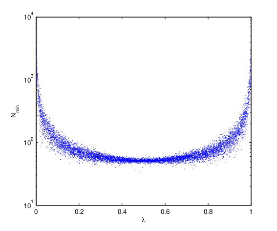
On the other hand, the ergodicity of the skew tent map permits to estimate the length of $P_{[0,1,\ldots,L-1]}$ by estimating the relative frequency of the $\pi=[0,1,\ldots,L-1]$ in a typical sharp orbit of the map —or, as we intent, in a typical coarse-grained orbit. In the latter case, the choice for the parameter $N$, the width of the sliding window down the Gray codes (Sect. V), must be also analyzed. The minimum value of $N$ to get a good reconstruction of the $\lambda$-DF of the order patterns, $N_{min}$, depends on the precision of the arithmetic used, but it also depends on the Lyapunov exponent of the map. If floating point double-precision arithmetic is implemented, then $N_{min}$ can be determined as function of $\lambda$ by comparing pairs of symbolic sequences generated from the same initial condition and control parameters $\lambda_{1}$ and $\lambda_{2}$ such that $|\lambda_{2}-\lambda_{1}|$ equals the spacing of floating point numbers. As it is shown in Fig. 10, the value of $N_{min}$ increases with the Lyapunov exponent for the skewed tent map.

Summing up, the estimation of the control parameter $\lambda\in(0,1)$ of the skew tent map $f_{\lambda}$, Eq. (5), can be done by counting and normalizing the occurrences of the order pattern $[0,1,...,L-1]$, ideally for $L=3$ or $4$, in a statistically significant sample of orbit segments of $f_{\lambda}$. This follows from the following properties: (i) $f_{\lambda}$ is ergodic for all $\lambda$, and (ii) the $f_{\lambda}$-invariant measure of $P_{[0,1,...,L-1]}$ (in this case, the length of the interval $P_{[0,1,...,L-1]}$) depends bijectively on $\lambda$. In a practical context though, finite precision machines are used, and this entails, in general, numerical degradation, this meaning that the computed orbits, whether of chaotic or non-chaotic maps, depart from the real ones. In the case of a very long orbit of a chaotic map, the deviation of the numerical simulation (locally measured by the Lyapunov exponent of the map) will be severe; in such cases, it is preferable to have many shorter orbits instead. Even worse, all orbits computed with finite precision are eventually periodic. This distortion of the dynamics, due to finite numerical precision and dependence on initial conditions, implies the general impossibility of obtaining orbits and invariant measures in an exact way. As a matter of fact, all this carries over to symbolic dynamics.

To verify this issue in the case of coarse-grained orbits, a sample of Gray codes of the skew tent map, each one with the same length but with a different initial condition, was generated for every value of $\lambda$. The underlying sharp orbits were computed with double precision floating point arithmetic. From this sample of Gray codes, the corresponding $\lambda$-DFs of the order patterns of length $L=4$ were obtained. The $\lambda$-DF of the order pattern $[0,1,2,3]$ ($\#0$ for short) was calculated as the mean value of the $\lambda$-DFs obtained from the various initial conditions. This average value is compared to the exact $\lambda$-DF, $\phi_{4}(\lambda)=\lambda^{2}/(2-\lambda)$, in Fig. 11, along with the corresponding standard deviation.

Fig. 11 spells out that, in the context of finite precision computation, the perfect recovery of the control parameter value using the $\lambda$-DF of order pattern $\#0$, is not feasible in general if one can only resort to Gray codes. However, it is possible to locate $\lambda$ up to an uncertainty interval. The width of this interval can be upper bounded by the standard deviation of the $\lambda$-DF of the order pattern $\#0$ since, according to Fig. 11, it is bigger than the average error in the estimation of $\phi_{4}(\lambda)$ for every value of $\lambda$ . Therefore, the estimation of the control parameter comprises two stages:

1. 1.

   An estimation of $\lambda$ is performed by dividing the given Gray code, $\left\{g_{i}\right\}_{i=0}^{M-1}$, $g_{i}\in\{0,1\}$, into a large enough set of disjoint subsequences of length $N\gg 4$, say, $\left\{g_{k\cdot N+i}\right\}_{i=0}^{N-1}$ for $k=0,1,\ldots,K=\left\lfloor M-N\right\rfloor-1$. For each such binary subsequence, a value of $\phi_{4}(\lambda)$ is then computed as the relative frequency of the order pattern $[0,1,2,3]$ using, of course, the Gray ordering (Sect. IV). Let $\bar{x}$ be the mean value of the resulting $\phi_{4}(\lambda)$’s. From $\phi_{4}(\lambda)=\lambda^{2}/(2-\lambda)$, Eq. (6), it follows that the control parameter is estimated as

   $$\hat{\lambda}=\phi_{4}^{-1}(\bar{x})=\frac{-\bar{x}+\sqrt{\bar{x}^{2}+8\bar{x}}}{2}.$$

   (14)

2. 2.

   If $\sigma$ is the standard deviation of the $\phi_{4}(\lambda)$ sampling, then

   $$\lambda\in(\phi_{4}^{-1}(\bar{x}-\sigma),\phi_{4}^{-1}(\bar{x}+\sigma)).$$

   (15)

The specifics of this procedure refers to the skew tent map, but the general strategy is the same, once a bijective $\lambda$-DF of an order pattern is exactly known.

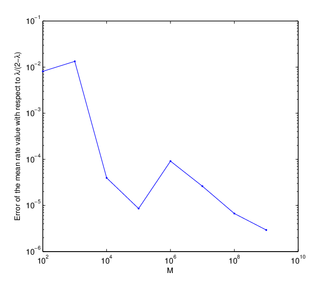
In order to establish the accuracy of the procedure, some numerical simulations with the skew tent map were done. For every value of the control parameter, a group of $100$ different initial conditions were used in the generation of the corresponding Gray codes. For each of these binary sequences, the control parameter $\lambda$ was estimated as just explained. The mean error of the estimation is shown in Fig. 12. The average error lies always above $10^{-4}$, and can only be reduced by the implementation of the procedure with extended-precision arithmetic libraries. To prove this claim, the case of the symmetric tent map, i.e., the skew tent map for $\lambda=1/2$, will be now considered. For the symmetric tent map the arithmetic is exact. Indeed, if $0.x_{0}x_{1}...x_{M}$, $x_{i}\in\{0,1\}$, is the expansion to base $2$ of $x\in[0,1]$, i.e.,

(numbers with finite binary expansions are called dyadic rationals), then the action of the symmetric tent map amounts to a zero-bit dependent left shift, to wit:

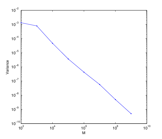
where $x_{n}^{\ast}=1-x_{n}$. Therefore, if $x\in[0,1]$ is represented with $M$ bits and $x_{M}=1$, the orbit of $x$ collapses to $0$ after $M$ iterations of $f_{1/2}$, so $M$ can be considered the effective length of the orbits to be used in an estimation of $\lambda=1/2$. For $L=3,$ the relative frequency of the order pattern $\#0$ ($[0,1,2]$ in this case) was determined for a large set of random initial conditions $x$ and increasing orbit lengths $M$. The convergence in average of this relative frequency to $\phi_{3}(1/2)=1/3$ (see Eq. (10)) as $M$ increases, is confirmed by Fig. 13. At the same time, the variance of the estimation steadily reduces with $M$, as shown in Fig. 14. In other words, a higher precision of the arithmetic used in orbit generation and greater samples for the subsequent control parameter estimation, clearly improves the results.

We conclude that the inaccuracies exposed above in our method to recover the control parameter of maps of $\mathcal{F}_{2}$, based on the order patterns of their coarse-grained orbits (specifically, in form of Gray codes), are due to the shortcomings of finite precision arithmetic and finite statistical sampling, but are not inherent to the method —as proved with the symmetric tent map.

In this paper it was shown how to rebuild the $\lambda$-DFs of order patterns from Gray codes, the scope being the estimation of the parameter $\lambda$. Gray codes are the 0-1 sequences that result from the symbolic dynamic of unimodal maps with respect to the left-right partition of the state space introduced by the critical point. We have analyzed the $\lambda$-DFs of the order patterns of two unimodal parametric maps: the logistic map (as representative of the subclass $\mathcal{F}_{1}$) and the skew tent map (as representative of the subclass $\mathcal{F}_{2}$). In the case of the logistic map, it turns out that this technique can hardly deliver, on account of the complex and many-to-one relation between $\lambda$ and those $\lambda$-DFs. On the contrary, this relationship is simple, one-to-one, and analytically known for $\pi=[0,1,...,L-1]$ in the case of the skew tent map. Our method improves previous proposals for parameter estimation of unimodal maps in that a knowledge of the critical point value is not needed. However, it demands high computational precision and large amounts of data; in this regard, we recommend the use of extended-precision libraries for good estimations. In the ideal case of arbitrarily high precision, the estimated value of the control parameter is arbitrarily close to the real one.

The work described in this paper was supported by Ministerio de Educación y Ciencia of Spain, research grant SEG2004-02418, CDTI, Ministerio de Industria, Turismo y Comercio of Spain in collaboration with Telefónica I+D, Project SEGUR@ with reference CENIT-2007 2004, CDTI, Ministerio de Industria, Turismo y Comercio of Spain in collaboration with SAP, project HESPERIA (CENIT 2006-2009), and Ministerio de Ciencia e Innovación of Spain in collaboration, project CUCO (MTM2008-02194).

References

- [1] N. Metropolis, M. Stein and P. Stein, “On the limit sets for transformations on the unit interval,” Journal of Combinatorial Theory (A) 15, 25–44 (1973).
- [2] L. Wang and N. D. Kazarinoff, “On the universal sequence generated by a class of unimodal functions,” Journal of Combinatorial Theory, Series A 46, 39–49 (1987).
- [3] G. Alvarez, M. Romera, G. Pastor and F. Montoya, “Gray codes and 1D quadratic maps,” Electronic Letters 34, 1304–1306 (1998).
- [4] J. M. Amigó, L. Kocarev and J. Szczepanski, “Order patterns and chaos,” Physics Letters, Section A: General, Atomic and Solid State Physics 355, 27–31, cited By (since 1996): 6 (2006).
- [5] D. L. Kreher and D. R. Stinson, Combinatorial Algorithms; Generation, Enumeration & Search (CRC Press, 1998).
- [6] J. M. Amigó, S. Elizalde and M. B. Kennel, “Forbidden patterns and shift systems,” Journal of Combinatorial Theory, Series A 115, 485–504 (2008).
- [7] P. Walters, An Introduction to Ergodic Theory, vol. 79 of Graduate Texts in Mathematics (Springer-Verlag, New York, 1982).
- [8] J. M. Amigó, S. Zambrano and M. A. F. Sanjuán, “True and false forbidden patterns in deterministic and random dynamics,” Europhysics Letters 79, 50001–p1, –p5 (2007).
- [9] W. Beyer, R. Mauldin and P. Stein, “Shift-maximal sequences in function iteration: Existence, uniqueness and multiplicity,” J. Math. Anal. Appl. 115, 305–362 (1986).
- [10] T. Cusick, “Gray codes and the symbolic dynamics of quadratic maps,” Electronic Letters 35, 468–469 (1999).