Family Gauge Symmetry as an Origin of
Koide’s Mass Formula and
Charged Lepton Spectrum
TU–833
Dec. 2008
Koide’s mass formula is an empirical relation among the charged lepton masses which holds with a striking precision. We present a model of charged lepton sector within an effective field theory with family gauge symmetry, which predicts Koide’s formula within the present experimental accuracy. Radiative corrections as well as other corrections to Koide’s mass formula have been taken into account. We adopt a known mechanism, through which the charged lepton spectrum is determined by the vacuum expectation value of a 9–component scalar field . On the basis of this mechanism, we implement the following mechanisms into our model: (1) The radiative correction induced by family gauge interaction cancels the QED radiative correction to Koide’s mass formula, assuming a scenario in which the family gauge symmetry and weak gauge symmetry are unified at – TeV scale; (2) A simple potential of invariant under leads to a realistic charged lepton spectrum, consistent with the experimental values, assuming that Koide’s formula is protected; (3) Koide’s formula is stabilized by embedding symmetry in a larger symmetry group. Formally fine tuning of parameters in the model is circumvented (apart from two exceptions) by appropriately connecting the charged lepton spectrum to the boundary (initial) conditions of the model at the cut–off scale. We also disucss some phenomenological implications.
1 Introduction
Among various properties of elementary particles, the spectra of the quarks and leptons exhibit unique patterns, and their origin still remains as a profound mystery. Within the Standard Model (SM) of elementary particles, the origin of the masses and mixings of the quarks and leptons is attributed to their interactions with the (as yet hypothetical) Higgs boson. Namely, these are the Yukawa interaction in the case of the charged leptons and quarks, and possibly the interaction represented by dimension–5 operators in the case of the left–handed neutrinos. Even if these interactions will be confirmed experimentally in the future, since the couping constants of these interactions are free parameters of the theory, the underlying mechanism how the texture of these couplings is determined would remain unrevealed.
There have been many attempts to approach the mystery of the fermion masses by identifying empirical relations among the observed fermion masses and exploring underlying physics that would lead to such relations. In particular, Koide’s mass formula is an empirical relation among the charged lepton masses given by [1]
| (1) |
which holds with a striking precision. In fact, substituting the present experimental values of the charged lepton masses [2], the formula is valid within the present experimental accuracies. The relative experimental error of the left-hand side (LHS) of eq. (1) is dominated by ( is the experimental error of ) and is of order . A simple mnemonic of the relation (1) is that the angle between the two vectors and equals [3].
Given the remarkable accuracy with which Koide’s mass formula holds, many speculations have been raised as to existence of some physical origin behind this mass formula [4, 3, 5, 6, 7, 8, 9]. Despite the attempts to find its origin, so far no realistic model or mechanism has been found which predicts Koide’s mass formula within the required accuracy. The most serious problem one faces in finding a realistic model or mechanism is caused by the QED radiative correction [7]. Even if one postulates some mechanism at a high energy scale that leads to this mass relation, the charged lepton masses receive the 1–loop QED radiative corrections given by
| (2) |
and denote the running mass defined in the modified–minimal–subtraction scheme ( scheme) and the pole mass, respectively; represents the renormalization scale. It is the pole mass that is measured in experiments. Suppose (or the corresponding Yukawa couplings ) satisfy the relation (1) at a high energy scale . Then do not satisfy the same relation [6, 7]: Eq. (1) is corrected by approximately 0.1%, which is 120 times larger than the present experimental error. Note that this correction originates only from the term of eq. (2), since the other terms, which are of the form , do not affect the relation (1). This is because, the latter corrections only change the length of the vector but not the direction. We also note that results from the fact that plays a role of an infrared (IR) cut–off in the loop integral.
The 1–loop weak correction is of the form in the leading order of expansion; the leading non–trivial correction is whose effect is smaller than the current experimental accuracy. Other radiative corrections within the SM (due to Higgs and would-be Nambu–Goldstone bosons) are also negligible.
Thus, if there is indeed a physical origin to Koide’s mass formula at a high energy scale, we need to account for a correction to the relation (1) that cancels the QED correction. Since such a correction is absent up to the scale of to our present knowledge, it must originate from a higher scale. Then, there is a difficulty in explaining why the size of such a correction should coincide accurately with the size of the QED correction which arises from much lower scales. There are also other less serious, but important questions that are often asked: (1) Why do not quark masses satisfy the same or a similar relation? (2) In Koide’s formula the three lepton masses appear symmetrically. Then why is there a hierarchy among these masses, ? If there is indeed a physical origin to Koide’s mass formula, there must be reasonable answers to all of these questions.
Among various existing models which attempt to explain origins of Koide’s mass formula, we find a class of models particularly attractive [10, 13]. These are the models which predict the mass matrix of the charged leptons to be proportional to the square of the vacuum expectation value (VEV) of a 9–component scalar field (we denote it as ) written in a 3–by–3 matrix form:
| (3) |
Thus, is proportional to the diagonal elements of in the basis where it is diagonal. The VEV is determined by minimizing the potential of scalar fields in each model. Hence, the origin of Koide’s formula is attributed to the specific form of the potential which realizes this relation in the vacuum configuration. Up to now, no model is complete with respect to symmetry: Every model requires either absence or strong suppression of some of the terms in the potential (which are allowed by the symmetry of that model), without justification.
In this paper, we study possible connections between family (horizontal) gauge symmetries and Koide’s formula and the charged lepton spectrum. These will be discussed within the context of an effective field theory (EFT) which is valid below some cut–off scale. In particular we address the following points:
- (i)
We propose a possible mechanism for cancellation of the QED radiative correction to Koide’s mass formula.
- (ii)
We propose a mechanism that produces the charged lepton spectrum, which is hierarchical and approximates the experimental values, under the assumption that Koide’s formula is protected by some other mechanism.
- (iii)
We present a model of charged lepton sector based on family gauge symmetry, incorporating the mechanisms (i)(ii). A new mechanism that stabilizes Koide’s formula is incorporated in this model.
(Among these, we have reported the main point of (i) separately in [11].)
In our study we adopt the mechanism eq. (3) for generating the charged lepton masses at tree level of EFT, for the following reasons. First, the mechanism allows for transparent and concise perturbative analyses of models, which is crucial in keeping radiative corrections under control. This may be contrasted with models with other mass generation mechanisms, such as dynamical symmetry breaking or composite lepton models, which typically involve strong interactions. Secondly, since is renormalized multiplicatively, the structure of radiative corrections becomes simple, as opposed to cases in which VEVs of more than one scalar fields contribute to the charged lepton spectrum. In short, this type of mass generation mechanism is pertinent to serious analyses of radiative corrections to Koide’s formula, which is a distinguished aspect of this study.
We alert in advance that we do not solve the hierarchy problem or fine tuning problem of the electroweak scale. We cannot explain how to stabilize the electroweak symmetry–breaking scale against other higher scales included in our model. Solution to this problem is beyond the scope of this paper.
The paper is organized as follows. In Sec. 2, we explain philosophy of our analysis using EFT and argue for its validity and usefulness. We also give a brief overview of the ideas presented in this paper. In Sec. 3, we explain the mechanism for cancelling the QED corrections to Koide’s formula. In Sec. 4, we present a potential for generating a realistic charged lepton spectrum, assuming that Koide’s formula is protected. In Sec. 5, we analyze a minimal potential whose vacuum corresponds to a desired lepton spectrum. In Sec. 6, we extend the potential by including another field. In Sec. 7, we introduce a higher–dimensional operator which generates the lepton masses and compute corrections to Koide’s formula. In Sec. 8, we discuss the energy scales and unsolved questions in our model. In Sec. 9, we discuss phenomenological implications of our model. In Sec. 10 summary and discussion are given. Technical details are collected in Appendices.
2 EFT Approach and Brief Overview of the Model
Throughout this paper, we consider an EFT which is valid up to some cut–off scale denoted by . In this EFT, we assume that the charged lepton masses are induced by a higher–dimensional operator
| (4) |
(or by other similar operators, as will be described later). Here, denotes the left–handed lepton doublet of the –th generation; denotes the right–handed charged lepton of the –th generation; denotes the Higgs doublet field. They are respectively assigned to the standard representations of the SM gauge group. By contrast, a 9–component scalar field is absent in the SM and a singlet under the SM gauge group. We suppressed all the indices except for the generation (family) indices . (Summation over repeated indices is understood throughout the paper unless otherwise stated.) The dimensionless Wilson coefficient of this operator is denoted as . Once acquires a VEV, the operator will effectively be rendered to the Yukawa interactions of the SM; after the Higgs field also acquires a VEV, with GeV, the operator will induce the charged–lepton mass matrix of the form eq. (3) at tree level:
| (5) |
For a moment, let us assume that the dimension–4 Yukawa interactions are prohibited by some mechanism. This will be imposed explicitly by a symmetry in our model to be discussed through Secs. 3–9.
We now explain philosophy of our analysis using EFT. Conventionally a more standard approach for explaining Koide’s mass formula has been to construct models within renormalizable theories. Nevertheless, the long history since the discovery of Koide’s formula shows that it is quite difficult to construct a viable renormalizable model for explaining Koide’s relation. It is likely that we are missing some essential hints to achieve this goal, if the relation is not a sheer coincidence. In this paper we will show that, within EFT, explanation of Koide’s formula is possible by largely avoiding fine tuning of parameters. Consistency conditions (with respect to symmetries of the theory) can be satisfied relatively easily in EFT, or in other words, they can be replaced by reasonable boundary conditions of EFT at the cut–off scale without conflicting symmetry requirements of the theory. (See Sec. 5.) Even under this less restrictive theoretical constraints, we may learn some important hints concerning the relation between the lepton spectrum and family symmetries. These are the role of specific family gauge symmetry in canceling the QED correction, the role of family symmetry in stabilizing Koide’s mass relation, or the role of family symmetry in realizing a realistic charged lepton spectrum consistently with experimental values. These properties do not come about separately but are closely tied with each other. These features do not seem to depend on details of more fundamental theory above the cut–off scale but rather on some general aspects of family symmetries and their breaking patterns. Thus, we consider that our approach based on EFT would be useful even in the case in which physics above the scale is obscure and may involve some totally unexpected ingredients —– as it was the case with chiral perturbation theory before the discovery of QCD.
Before discussing radiative corrections within EFT, one would be worried about effects of higher–dimensional operators suppressed in higher powers of . Indeed, using the values of tau mass and the electroweak symmetry breaking scale , one readily finds that ( are the diagonal elements of in the basis where it is diagonal). Hence, naive dimensional analysis indicates that there would be corrections to Koide’s formula of order 10% even at tree level. We now argue that this is not necessarily the case within the scenario under consideration. We may divide the corrections into two parts. These are (i) corrections to the operator of eq. (4) (the operator which reduces to the SM Yukawa interactions after is replaced by its VEV), and (ii) corrections to the VEV of .
Concerning the corrections (i), we may consider the following example.** * A similar mechanism is used in [10, 12] to induce ; corrections by higher–order terms in have not been discussed, however. Suppose that the operator is induced from the interactions
| (6) |
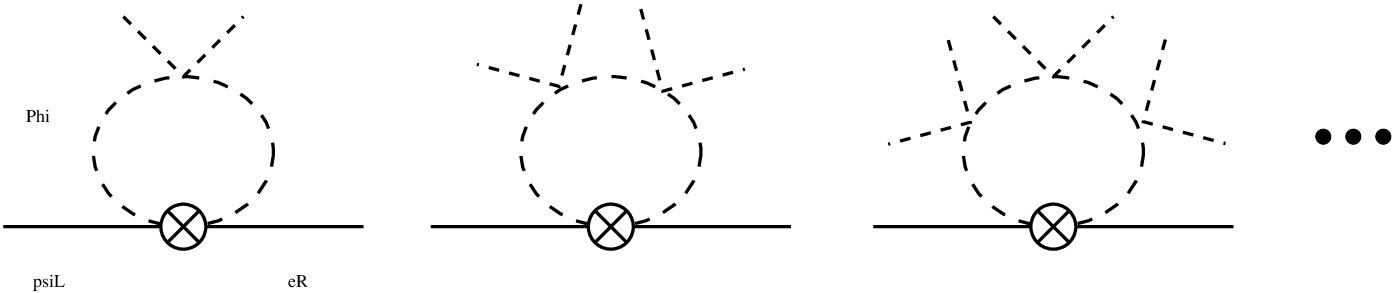
through the diagram shown in Fig. 1, after fermions and have been integrated out.

Fermions and are assigned to appropriate representations of the SM gauge group such that the above interactions become gauge singlet. For instance, in the case that , and , one finds, by computing the mass eigenvalues,†† † Since the values of and are known, once we choose the values of and , the value of will be fixed. Then the mass eigenvalues corresponding to the SM charged leptons can be computed in series expansion in the small parameters , and . that the largest correction to the lepton spectrum eq. (5) arises from the operator ; its contribution to the tau mass is . This translates to a correction to Koide’s relation of , due to the suppression factor . Thus, this is an example of underlying mechanism that generates the operator without generating higher–dimensional operators conflicting the current experimental bound. If we introduce even more (non–SM) fermions to generate the leading–order operator , one can always find a pattern of spectrum of these fermions, for which higher–dimensional operators are sufficiently suppressed, since the number of adjustable parameters increases. (Another example of underlying mechanism may be the one proposed in [8], based on the idea of [14].) In general, sizes of higher–dimensional operators depend heavily on underlying dynamics above the cut–off scale.
Let us restrict ourselves within EFT. If we introduce only the operator , by definition this is the only contribution to the charged lepton spectrum at tree level. Whether loop diagrams induce higher–dimensional operators which violate Koide’s relation is an important question, and a detailed analysis is necessary. This is the subject of the present study, where the result depends on the mechanisms how Koide’s formula is satisfied and how the charged lepton spectrum is determined, even within EFT. The conclusion is as follows. Within the model to be discussed in Secs. 3–8, the class of 1–loop diagrams shown in Fig. 2 do not generate operators that violate Koide’s relation sizably; see Sec. 7. (There is another type of 1–loop diagrams that possibly cancels the QED correction; see Sec. 3.) In fact, we do not find any loop–induced higher–dimensional operators, which violate Koide’s relation in conflict with the current experimental bound.
Concerning the corrections (ii), in our analysis we introduce specific family gauge symmetries and their breaking patterns such that the corrections (ii) are suppressed.
Since the above example of underlying mechanism that suppresses higher–dimensional operators is simple, and since suppression of loop–induced corrections within EFT provides a non–trivial cross check of theoretical consistency, we believe that our approach based on EFT has a certain justification and would be useful as a basis for considering more fundamental models.
In the rest of this section, we present a brief overview of the basic ideas of the analysis to be given through Secs. 3–8, in order to facilitate reading. Our analysis starts from investigating a possibility that the radiative correction generated by a family gauge symmetry cancels the QED correction to Koide’s formula (Sec. 3). We find that family gauge symmetry has a unique property in this regard. In fact, if and are assigned to mutually conjugate representations of this symmetry group, the radiative correction has the same form as the QED correction with opposite sign. In particular, if the gauge coupling of family symmetry satisfies the relation , both corrections cancel. We speculate that this relation would be realized within a scenario in which family gauge symmetry is unified with gauge symmetry at – TeV scale, although we need to fine tune the unification scale within an accuracy of factor 3.
The non–trivial form of the radiative correction by the gauge interaction is dictated by the symmetry and its breaking pattern induced by the VEV . In particular, multiplicative renormalizability of ensures that the correction to Koide’s formula is independent of the renormalization scale of the effective potential of . Namely, the charged lepton pole masses are determined, up to a common multiplicative constant, directly by the form of the effective potential renormalized at an arbitrary high scale (), and we may ignore the QED and radiative corrections altogether. For our purpose, it is most convenient to take this scale to be . In this part of our analysis, we assume that can be brought to a diagonal form by symmetry transformation, and also that Koide’s relation for the diagonal elements,
| (7) |
is satisfied.
In the second step, we search for an effective potential for which the eigenvalues of satisfy the relation (7) and reproduce the experimental values of the mass ratios (Secs. 4 and 5). If we choose the renormalization scale to be , radiative corrections to the effective potential essentially vanish within EFT, or in other words, the form of the effective potential at this scale is determined by physics above the scale as boundary (initial) conditions of EFT. Hence, our goal is to find an effective potential which satisfies the boundary conditions without conflicting symmetry requirements of the theory. Although it may seem an easy task, it still involves fairly non-trivial analyses.
We impose family symmetry as a symmetry of EFT. The motivation of this choice is that it is the symmetry possessed by the simplest higher–dimensional operator analyzed in the first step. It turns out, however, that this symmetry is not large enough to constrain the form of the effective potential sufficiently. We therefore further assume a symmetry enhancement. Namely, we assume that above the cut–off scale there is an gauge symmetry, and this symmetry is spontaneously broken to below the cut–off scale. The symmetry is motivated by a geometrical interpretation of Koide’s relation eq. (7). Within this scenario, we still need to introduce an additional scalar field in order to realize a desirable vacuum configuration. Thus, we analyze the vacuum of the general potential of and . (Details of the analysis are rather technical.) The conclusion is that in a finite region of the parameter space of the potential, Koide’s relation is satisfied by the eigenvalues of . Furthermore, the eigenvalues can be made consistent with the experimental values of the charged lepton masses without fine tuning of parameters. These are realized in the case that certain hierarchical relations among the parameters of the potential are satisfied, and these relations do not conflict the requirement of the assumed symmetry and symmetry enhancement. We speculate on possible physics scenario above the cut–off scale that may lead to (part of) these hierarchical relations.
So far, these desirable features are satisfied by the eigenvalues of . There remains, however, a problem that cannot be brought to a diagonal form by the symmetry transformation, and this contradicts the assumption made in the first step. To remedy this difficulty, we introduce yet another field such that, with an appropriate potential with , it can generate an appropriate higher–dimensional operator necessary to produce the charged lepton masses. (Secs. 6 and 7.) Although the potential and the higher–dimensional operator involving do not conflict the requirement of the assumed symmetry and symmetry enhancement, these would be the most unsatisfactory part of our model. This is because it is difficult to speculate any plausible scenario above the cut–off scale, which would lead to these potential and higher–dimensional operator.
With all these setups, it is possible to compute the radiative corrections which are induced by the diagrams shown in Fig. 2. Due to the specific form of the effective potential of and , corrections to Koide’s formula turn out to be quite suppressed, as long as the aforementioned hierarchical conditions between parameters of the potential are satisfied. As already mentioned, this serves as a non–trivial consistency check of the model as an EFT.
3 Radiative Correction by Family Gauge Interaction

In this section we introduce family gauge symmetries and consider radiative corrections to the mass matrix eq. (5) by the family gauge interaction. First we consider the case, in which the family gauge group is and both and are assigned to the (fundamental representation) of this symmetry group. We readily see, however, that with this choice of representation, Koide’s formula will receive a severe radiative correction unless the family gauge interaction is strongly suppressed. In fact, the 1–loop diagram shown in Fig. 3 induces an effective operator
| (8) |
hence corrections universal to all the charged–lepton masses, , are induced. This is due to the fact that the dimension–4 operator is not prohibited by symmetry. Here, denotes the gauge coupling constant of the family gauge interaction. As noted above, corrections which are proportional to individual masses do not affect Koide’s formula; oppositely, the universal correction violates Koide’s formula rather strongly. In order that the correction to Koide’s formula cancel the QED correction, a naive estimate shows that should be order , provided that the cut–off is not too large and that the above operator is absent at tree level. If exists at tree level, there should be a fine tuning between the tree–level and 1–loop contributions. The situation is similar if the family symmetry is and both and are in the , which is also a typical assignment in existing models. In these cases [15] we were unable to find any sensible reasoning for the cancellation between the QED correction and the correction induced by family gauge interaction, other than to regard the cancellation as just a pure coincidence. Hence, we will not investigate these choices of representation further.
In the case that is assigned to and to (or vice versa) of family gauge group, (i) the dimension–4 operator is prohibited by symmetry, and hence corrections universal to all the three masses do not appear; and (ii) marked resemblance of the radiative correction to the QED correction follows. We show these points explicitly in a specific setup.
We denote the generators for the fundamental representation of by (), which satisfy
| (9) |
is the generator of , hence it is proportional to the identity matrix, while () are the generators of . Here and hereafter, represent indices , while represent indices . The explicit forms of are given in Appendix A.
We assign to the representation , where stands for the representation and 1 for the charge, while is assigned to . Under , the 9–component field transforms as three ’s. Explicitly the transformations of these fields are given by
| (10) |
We assume that the charged–lepton mass matrix is induced by a higher–dimensional operator similar to in eq. (4). We further assume that can be brought to a diagonal form in an appropriate basis. Thus, in this basis , after and acquire VEVs, turns to the lepton mass terms as
where
When all are different, symmetry is completely broken by , and the spectrum of the gauge bosons is determined by .
Note that the operator in eq. (4) is not invariant under the transformations eq. (10). As an example of , one may consider
| (19) |
It is invariant under a larger symmetry , under which transforms as (). In this case, we need to assume, for instance, that the symmetry is gauged and spontaneously broken at a high energy scale before the breakdown of the symmetry, in order to eliminate massless Nambu–Goldstone bosons and to suppress mixing of the and gauge bosons. A more elaborate example of the higher–dimensional operator, which is consistent with the symmetry and satisfies eqs. (3) and (3), will be given in Sec. 7. In any case, the properties of given by eqs. (3) and (3) are sufficient for computing the radiative correction by the gauge bosons to the mass matrix, without an explicit form of .
 |
| (a) |
 |
| (b) |
|
|
| (c) |
We take the and gauge coupling constants to be the same:
| (20) |
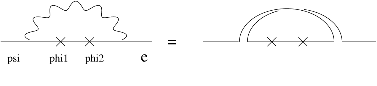
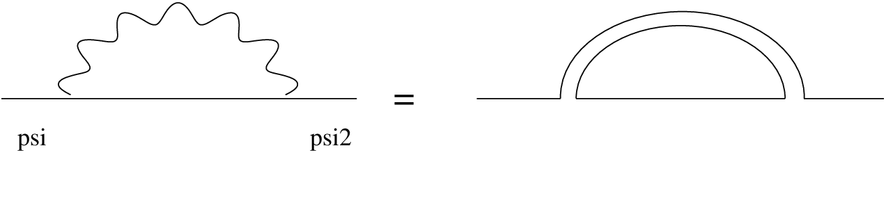
We compute the radiative correction in Landau gauge, which is known to be convenient for computations in theories with spontaneous symmetry breaking. From the diagrams shown in Figs. 4(a)(b)(c), we find
| (21) | |||
| (22) |
Here, is a constant independent of . The Wilson coefficient is defined in scheme. ’s are defined as follows: The VEV of at renormalization scale , given by eq. (3), is determined by minimizing the 1–loop effective potential in Landau gauge (although we do not discuss the explicit form of the effective potential in this section); is renormalized in scheme. We ignored terms suppressed by in the above expression. Note that the pole mass is renormalization–group invariant and gauge independent. Therefore, the above expression is rendered gauge–independent if we express in terms of gauge–independent parameters, such as coupling constants defined in on–shell scheme.
The coefficient of is determined by the sum of the anomalous dimension of the Wilson coefficient and twice of the wave–function renormalization of . (The former is gauge independent, while the latter is not.) The term originates from the role of the gauge boson masses as an IR cut–off of the loop integral, hence it reflects the spectrum of the gauge bosons. The sign in front of is opposite to that of the QED correction eq. (2), which results from the fact that and have the same QED charges but mutually conjugate (opposite) charges.
In Landau gauge, the diagrams in Figs. 4(b)(c) are finite and flavor independent, i.e. proportional to in terms of the family indices; hence they contribute only to the constant . Apart from this constant, the difference between the QED correction and the correction (21) resides in the factors
| (23) |
in the QED self–energy diagram and the diagram in Fig. 4(a), respectively. (No sum over is taken in the former factor.) One may easily identify the factor 2 difference in the coefficients of using the Fierz identity
| (24) |
From this identity, it follows that the operator is multiplicatively renormalized; see family charge flow in Fig. 4(a). denotes the mass matrix of the family gauge bosons. After diagonalization, one obtains the spectrum of family gauge bosons as
| (25) |
The mass eigenstates are labelled in the order of their masses, which are given by
Hence,
The form of the radiative correction given by eqs. (21) and (22) is constrained by symmetries and their breaking patterns. As the diagonal elements of the VEV, , are successively turned on, gauge symmetry is broken according to the pattern:
| (33) |
At each stage, the gauge bosons corresponding to the broken generators acquire masses and decouple. Furthermore, the vacuum and the family gauge interaction respect a global symmetry generated by
| (34) |
with
The operator after symmetry breakdown, eq. (3), is not invariant under this transformation but the variation can be absorbed into a redefinition of ’s. As a result, the lepton mass matrix has a following transformation property:
| (39) |
This is satisfied including the 1–loop radiative correction. The symmetry breaking pattern eq. (33) and the above transformation property constrain the form of the radiative correction to , where the constant is independent of . Note that in the argument of logarithm originate from the gauge boson masses, which are invariant under .
The universality of the and gauge couplings eq. (20) is necessary to guarantee the above symmetry breaking pattern eq. (33). One may worry about validity of the assumption for the universality, since the two couplings are renormalized differently in general. The universality can be ensured approximately if these two symmetry groups are embedded into a simple group down to a scale close to the relevant scale. There are more than one ways to achieve this. A simplest way would be to embed into . It is easy to verify that the of decomposes into under . Hence, the (second-rank antisymmetric representation) and of , respectively, include and .
Within the effective theory under consideration, the QED correction to the pole mass is given just as in eq. (2) with replaced by . Recall that corrections of the form do not affect Koide’s formula. Then, noting , one observes that if a relation between the QED and family gauge coupling constants
| (40) |
is satisfied, the 1–loop radiative correction induced by family gauge interaction cancels the 1–loop QED correction to Koide’s mass formula.
In fact, with the relation (40), cancellation holds for all the leading logarithms generated by renormalization group: the coefficient of of the QED correction is determined by the 1–loop anomalous dimension of the running mass, while the coefficient of of eq. (21) is determined by the anomalous dimension of the Wilson coefficient and twice of the wave–function renormalization of ; they are resummed in the same way by 1–loop renormalization group equations. The renormalization group evolution and the symmetry breaking pattern eq. (33) in the scale range across the family gauge boson masses dictate how ’s induced by family gauge interaction are resummed. The renormalization group evolution and the same symmetry breaking pattern in the QED sector dictate the resummation of the QED correction, in the scale range across the lepton masses. If cancel at 1–loop, dependences in all the leading logarithms also cancel. On the other hand, effects of the running of and do not cancel. It is related to the question which we stated in the Introduction: What are the relevant scales for the coupling constants in the relation (40)? The scale of is determined by the lepton masses, while the scale of is determined by the family gauge boson masses, which should be much higher than the electroweak scale.
Suppose the relation (40) is satisfied. Then
| (41) |
holds including the leading logarithms generated by the running of and ’s. This is valid for any value of . This means, if ’s satisfy
| (42) |
at some scale , Koide’s formula is satisfied at any scale . This is a consequence of the fact that is multiplicatively renormalized. Generally, the form of the effective potential varies with scale . If the relation (42) is realized at some scale as a consequence of a specific nature of the effective potential (in Landau gauge), the same relation holds automatically at any scale. Although these statements are formally true, physically one should consider scales only above the family gauge boson masses, since decoupling of the gauge bosons is not encoded in scheme. For our purpose, it is most appropriate to use eq. (41) to relate the charged lepton pole masses with the VEV at the cut–off scale, i.e. , which sets a boundary (initial) condition of the effective theory.
The advantages of choosing Landau gauge in our computation are two folds: (1) The computation of the 1–loop effective potential for the determination of becomes particularly simple (as well known in computations of the effective potential in various models); in particular there is no correction to the effective potential. (2) The lepton wave–function renormalization is finite; as a consequence, the diagrams in Figs. 4(b)(c) are independent of and independent of flavor. Due to the former property, there is no correction to the relation eq. (42) if it is satisfied at tree level. Due to the latter property, is determined essentially by the diagram in Fig. 4(a) and a simple relation to follows.
Let us comment on gauge dependence of our prediction. If we take another gauge and express the radiative correction in terms of , the coefficient of changes, and other non–trivial flavor dependent corrections are induced. Suppose the relation eq. (42) is satisfied at tree level.** * To simplify the argument we consider only those gauges in which tree–level vacuum configuration is gauge independent, such as the class of gauges considered in [16]. The VEV in another gauge receives an correction, which induces a correction to eq. (42) at . These additional corrections to at should cancel altogether if they are reexpressed in terms of the tree–level ’s which satisfy eq. (42), since the correction to the relation (42) vanishes in Landau gauge. General analyses of gauge dependence of the effective potential may be found in [17].
Now we speculate on a possible scenario how the relation (40) may be satisfied. Since the relevant scales involved in and are very different, we are unable to avoid assuming some accidental factor (or parameter tuning) to achieve this condition. Instead we seek for an indirect evidence which indicates such an accident has occurred in Nature. The relation (40) shows that the value of is close to that of the weak gauge coupling constant , since is close to . In fact, within the SM, approximates at scale – TeV. Hence, if the electroweak gauge group and the family gauge group are unified around this scale, naively we expect that
| (43) |
is satisfied. Since runs relatively slowly in the SM, even if the unification scale is varied within a factor of 3, Koide’s mass formula is satisfied within the present experimental accuracy. This shows the level of parameter tuning required in this scenario.
We may generalize our setup and see how the radiative correction alters. If and are assigned to and , respectively, the correction eq. (21) generalizes to
| (44) |
where is a flavor–independent constant. Thus, the form is maintained. This is not the case if we vary the charge of , which violates the breaking pattern of gauge symmetry eq. (33) strongly.†† † Even in the case in which only the charges of and are varied, this symmetry breaking pattern is violated but only softly through the gauge interaction of and . By contrast, varying the charge of affects the spectrum of the gauge bosons. The form is maintained in yet another generalization, in which symmetry is gauged. We introduce another field under . The symmetry transformations are given by , , , with , . We assume that with , and that the lepton masses are generated by a higher–dimensional operator
| (45) |
For the assignment and , the radiative correction reads
| (46) |
where and denote, respectively, the gauge couplings of the first and second symmetries.‡‡ ‡ If , can be embedded into . In this case, and can be assigned to the and of , respectively. The remaining , corresponding to the lepton number, is unbroken, so it may be taken as a global symmetry. Thus, the coefficient of varies in different setups. Accordingly the condition for the cancellation of the QED correction changes from eq. (40). We need to seek for other possible scenarios which lead to such conditions, or maybe to let the cancellation be a sheer coincidence. The level of fine tuning required for the coupling(s) is about 1% to meet the present expermental accuracy of Koide’s formula.
In the rest of this paper, we do not consider these generalizations. We adhere to eq. (40), assuming the scenario in which and gauge symmetries are unified at around – TeV. In this paper we do not construct a model which incorporates this unification scenario. We simply assume that this unification scenario is realized in the underlying full theory, in which the unification scale is at or around the cut–off scale of our effective theory; we further assume that the hierarchy between and is mild; see discussions in Secs. 2 and 8.
4 Potential Minimum and Charged Lepton Spectrum
The analysis in the previous section indicates relevance of the family gauge symmetry in relation to the charged lepton spectrum and Koide’s mass formula. In this section we study the potential of invariant under this family symmetry and its classical vacuum. In particular, we propose a mechanism for generating a realistic charged lepton spectrum, assuming that Koide’s mass relation is protected. For later convenience, we express components of using , defined in eqs. (9) and (A), as the basis:
| (47) |
In general takes a complex value.
The largest symmetry that can be imposed on the higher–dimensional operator is . [An example is given in eq. (45).] We may consider the potential of consistent with this symmetry, allowing only operators with dimension 4 or less. A general analysis shows that, for any choice of the parameters (couplings) of this potential, the classical vacuum , after its diagonalization, does not satisfy the relation (42) [18]. Namely, there is no classical vacuum that leads to Koide’s mass formula. If we impose a smaller symmetry on the potential of , it is possible to tune the parameters in the potential and realize the relation (42) as well as a realistic charged lepton spectrum. We were, however, unable to find a sensible reasoning for tuning the parameters with an accuracy necessary to realize Koide’s mass formula.

We may reverse the argument partially and search for a realistic vacuum within a restricted set of configurations. Namely, in view of the high accuracy with which Koide’s mass formula is realized in Nature, it may make sense to assume that this mass relation is protected by some mechanism. (An example of such a mechanism will be given in the next section.) We assume that the vacuum configuration satisfies
| (48) |
in an appropriate basis allowed by the symmetry. In this case, the relation (42) is satisfied by the eigenvalues of [10]; see Fig. 5. Then we minimize the potential of within the configurations which satisfy this condition. Eq. (48) imposes one condition among the three masses of leptons. Apart from the overall normalization of the spectrum, there remains only one free parameter, which should be fixed by minimizing the potential. Since the condition (48) or the relation (42) treats the three mass eigenvalues symmetrically, a priori it seems difficult to generate a hierarchical spectrum. If we impose the symmetry to the potential of , there is no vacuum corresponding to a realistic lepton spectrum. We find that in the case of the symmetry, a realistic spectrum follows from the vacuum of a simple potential.
In the rest of this section we study a classical vacuum of the potential of which is invariant under the transformation
| (49) |
Up to dimension 4, there are only 4 independent invariant operators. We parametrize the potential as
| (50) |
where
| (51) | |||
| (52) | |||
| (53) |
The 4 independent parameters , , and are real. These potentials are classified according to the symmetries: Since , is invariant under ; is invariant under ; is invariant under .
We assume the condition (48). When and , the configuration which minimizes under this condition corresponds to a charged lepton spectrum very close to the experimentally observed one. Let us describe the details of this configuration. Using the transformation (49), any can be brought to a form parametrized by 6 real parameters. Without loss of generality, we can choose as the real parameters, while are set to zero.** * Since any can be diagonalized by a bi–unitary transformation, , can be brought to an hermite matrix by a transformation as , i.e. . Noting that transforms as the of the diagonal subgroup , we may set using this transformation. Using a residual degree of freedom, which rotates as a real doublet of , we can set . Then it is straightforward (but cumbersome) to minimize the potential under the condition (48). One finds the global minimum at the configuration
where†† † is a real solution to the equation .
| (57) | |||
| (58) |
There are no other degenerate vacua except those which are connected to by the transformation (49). Note that there is a residual symmetry corresponding to the transformation
| (59) |
which keeps the above vacuum invariant. This is a subgroup of .
The three eigenvalues of are given by
| (60) |
The corresponding experimental values read
| (61) |
where . We pay particular attention to the value of , which approximates the corresponding experimental value with an accuracy of . Since the constraint (48) treats the three eigenvalues symmetrically, some kind of fine tuning should be inherent in this vacuum configuration corresponding to a hierarchical spectrum. Indeed, this is reflected to the fact that, if the value of is varied slightly from the above value under the condition (48), variations of and are fairly enhanced. (Note that the values of and are fixed by .) As a result, a tiny perturbation to the potential can bring all to be consistent with the experimental values. For instance, turning on with will achieve this. This feature is indifferent to details of perturbations: they can be any mixture of , higher–dimensional operators, and radiatively induced potentials (log potentials).
The following comparison may illustrate markedness of the above configuration. When this configuration is the zeroth–order vacuum, correct orders of magnitude of , , are reproduced if perturbations are sufficiently small. By contrast, when the zeroth–order value of is in less accurate agreement with the experimental value, a fine tuning of perturbative contributions is necessary even to reproduce the mass ratios with correct orders of magnitude.‡‡ ‡ For instance, if ( difference from the experimental value), and are predicted to be the same, .
We find it quite intriguing that the vacuum of such a simple potential, which respects the family symmetry, selects this particular value of very close to the realistic value. Noting the relation (41) between the lepton pole masses and the VEV of at high energy scales, the above feature may suggest that the potential takes a form at the cut–off scale .
At this stage, it is unclear what mechanism protects the condition (48). Furthermore, it is unclear why should be so much suppressed compared to , . Naively, one would expect that radiative corrections induce at least with a similar order of magnitude as . In the next section, we will present a possible mechanism or scenario to solve these problems (not completely but at least in such a way to circumvent fine tuning of parameters).
5 A Minimal Potential
In this section, we present a potential of scalar fields, possibly minimal in its content, which realizes , defined in eq. (4), at its classical vacuum. This is discussed within an effective theory which has family gauge symmetry, valid below the cut–off scale . The assignment to of the fields, which are already introduced in the previous sections, reads
| (62) |
with the transformation properties
| (63) | |||
| (64) |
Furthermore, we assume that above the cut–off scale there is an gauge symmetry and that this symmetry is spontaneously broken to below the cut–off scale.
Let us describe the assignment of the fields to the group . is assigned to ; its transformation is given by with a 9--by--9 unitary matrix** * For instance, is invariant under as well as . . is included in (the is the second–rank antisymmetric representation), which decomposes into after the symmetry breakdown; similarly is included in . is a singlet under .
In order to realize a desirable vacuum configuration, we introduce another field , which is in the representation (the is the second–rank symmetric representation) and is unitary. It can be represented by a 9–by–9 unitary symmetric matrix:
| (65) |
decomposes into after the symmetry breakdown. See Appendix B for the decomposition of under .
We may summarize the essence of how to realize a vacuum, which satisfies eq. (48), as follows. If the VEV of takes a value
| (66) |
an –invariant condition
| (67) |
reduces to the first condition in eq. (48) at . The second condition in eq. (48) can be realized by maximizing upon fixing the value of and imposing the first condition of eq. (48); see Appendix C.1. These conditions can be met at the classical vacuum of the potential of the scalar fields under consideration, with an appropriate choice of parameters in the potential. We may avoid fine tuning of the parameters, except for the one related to stabilization of the electroweak scale.
In what follows we do not discuss any details of the theory above the scale . Rather we use general properties of gauge symmetry to infer boundary conditions to be imposed at the scale . We also investigate boundary conditions at this scale required from the low–energy side phenomenologically, consistently with symmetry requirements.
We study the potential and its vacuum of the scalar fields, , and . First we analyze the potential of a specific form (or with a specific choice of parameters of the potential), which incorporates an essential part of our model. Later we extend the potential to more general forms. The potential we analyze reads
| (68) |
where and are defined in eqs. (51) and (53), respectively, and the other potentials are defined by
| (69) | |||
| (70) | |||
| (71) |
All the parameters of the potential, , , , , , , are taken to be positive. Note that since the field is unitary, it is dimensionless. The physical scale of its VEV is determined by the kinetic term of , which is normalized as . Thus, the physical scale of the VEV of is . We choose to be much smaller than (the scale of ), such that the spectrum of the family gauge bosons is determined predominantly by . (See discussion in Sec. 8.)
One may verify the following properties of the potential:
- •
The global minimum of is at , defined by eq. (66). Degenerate configurations are only those which are connected to by the transformation (the symmetry transformation of ).
- •
is minimized if eq. (67) holds. This equation reduces to the condition in the case that .
- •
If , up to a term that can be absorbed in :
(72) - •
If the constraints and are imposed, is minimized when ’s have a common phase , namely for all ; see Appendix C.1.
- •
, defined by eq. (4), is the classical vacuum of under the constraints , and .
- •
If the constraints and are imposed, the first derivative of vanishes,†† † It can be shown, for instance, from the invariance of both and under the transformation eq. (59) and two transformations given by with and . , at . This is not trivial: In general there may be a non–zero derivative in an imaginary direction, since is determined assuming .
- •
All terms in except is invariant under , while the variation of is positive semi–definite at . Namely, if , ; see Appendix C.2.
Due to these properties, the classical vacuum of in the limit is given by and up to a transformation, provided that exceeds a critical value to assure the reality condition on (up to a common phase):
| (73) |
We note that the definition of should be modified, including the effect of , from eq. (58) to
| (74) |
The operators and , whose couplings need to be suppressed, are non–invariant under . This is a key property of our model which allows us to circumvent fine tuning, as we will discuss shortly. As far as the charged lepton masses are concerned, the phase can be removed by redefining the phases of and . Hence, we set in the following analysis for simplicity.‡‡ ‡ The degeneracy of the vacua parametrized by originates from an accidental global symmetry of the potential , under which the overall phase of is rotated independently of . The degeneracy will be lifted if we include in the potential operators which break this accidental symmetry.
The and corrections to the vacuum configuration can be computed. In an appropriate basis, these are given by
| (75) | |||
| (76) | |||
| (77) | |||
| (78) | |||
| (79) |
where
| (80) |
and ’s are given by eq. (60). Hence, violation of Koide’s mass formula is expected to be or , where represents or . The explicit expression of the charged lepton spectrum including the above corrections depends on the precise form of the higher–dimensional operator which generates the lepton masses. Naively one expects that should be satisfied, in order to meet the experimental accuracy of Koide’s formula. [Compare with the estimates below eq. (121).]
Next we consider the potential of and in general and examine conditions necessary for realizing and . Noting that is unitary, the potential invariant under can be written as
| (81) |
When the coefficients are appropriately chosen (without fine tuning), can have a minimum at and . These are satisfied by and .
All the other operators are non–invariant under . We separate them into three categories: those which depend only on (), those which depend only on (), and those which depend on both and (). Requirements to each of them are as follows:
- •
We can show that the first derivative of vanishes at if invariance is preserved; see Appendix C.4. This means that, assuming invariance, can be the global minimum of in a certain domain of the parameter space (spanned by the parameters in ), without fine tuning of parameters.§§ § One example is the case in which gives a dominant contribution in , although other operators need not be suppressed by orders of magnitude. This is because, contributions of other operators cannot create a non–zero derivative at , and the position of the global minimum is altered only if their contributions are large enough to create a global minimum at another configuration.
- •
Up to dimension 4, consists only of and ; see Sec. 4. Since effects of higher–dimensional operators are expected to be suppressed, will be minimized at if and . Here, and represent typical magnitudes of the second derivatives of and , respectively, at their minima.
- •
The contribution of needs to be suppressed as compared to those of and . If we can treat as a perturbation, we may substitute and in the lowest–order approximation. Then becomes dependent only on and . The role of the operators dependent only on is similar to ; their total contribution should not be too small compared to that of and should enforce the reality condition on ; c.f. eq. (73). The role of the operators dependent on is similar to ; in order to suppress corrections to the lepton spectrum, contributions of these operators need to be suppressed compared to that of .
Thus, under appropriate conditions, can be realized with a more general potential than the specific potential eq. (68). Coefficients of certain operators need to be suppressed compared to the others. One may estimate typical orders of magnitudes of hierarchies required in the constraints, from the analysis of the specific potential , which serves as a reference case. Moreover, in principle it is straightforward to compute corrections to the vacuum configuration similar to eqs. (75)–(79) for a more general potential.
Let us comment on invariance. We may assume that either invariance is broken explicitly (but weakly) or it is broken spontaneously. In the former case, since there is no observed asymmetry in the lepton sector, we may assume effects of the explict breaking are very small and will not affect our argument given above significantly. In the latter case, since asymmetry resides only in the Yukawa interaction in the SM, we may attribute the Kobayashi-Maskawa phase to the VEV of the scalar field, which is presumably existent to give masses to the quarks, while keeping all the interactions in the effective theory –invariant. As we do not discuss quark sector at all in this paper, this argument is rather ambiguous. In passing, we note that all the operators in the potential [eq. (68)] are –invariant; see Appendix C.3 for the transformations.
Furthermore, the Higgs field needs to be incorporated in the potential. Since is a singlet under , it can be included effectively by replacing the coefficients of the operators in the above discussion by functions (polynomials) of , e.g. . Hence, the conditions on the coefficients are the same as above when evaluated at . On the other hand, the VEV of is determined from the same potential after substituting and , whose expansion about the minimum should take a form .
It is appropriate to regard the conditions discussed above as those to be imposed on the Wilson coefficients in the effective potential (in Landau gauge) renormalized at the cut–off scale . Recall that, as we discussed in Sec. 3, we may relate the charged lepton spectrum directly to the vacuum configuration of the effective potential at . The advantage of choosing is that certain fine tuning can be avoided in this way. Let us describe how it works.
According to the argument above, is required to be much smaller than or in order to suppress corrections to Koide’s formula. Furthermore, in Sec. 4 we have seen that should be much smaller than to generate a realistic charged lepton spectrum. Hence, and should be quite small, of order or less. On the other hand, the 1–loop correction by family gauge interaction to the effective potential induces . This indicates that a natural size of is order or larger within the effective theory, assuming the relation (40). Thus, in order to realize , a fine tuning of seems to be requisite (provided magnitudes of and are moderate). This argument, however, does not apply at the cut–off scale : Since symmetry forbids and in the theory above the scale , both and are expected to be suppressed at in the theory. They are determined by the matching conditions at . Radiative corrections within the effective theory essentially do not exist at this scale.
Another advantage of choosing in the effective potential is that symmetry breaking effects on are also expected to be suppressed. In other words, the wave function renormalizations are common to , and , to a good approximation. It helps to keep the first condition of eq. (48) precise, which follows from eqs. (66) and (67).
The sizes of Wilson coefficients of operators non–invariant under at depend on the dynamics how the breakdown of gauge symmetry occurs in the theory above the scale . For example, one can imagine cases in which these operators are proportional to (powers of) a VEV of some scalar field which breaks symmetry. Then, an operator whose dimension is would have a coefficient of order , where is a combination of coupling constants, is a typical scale of the scalar VEV, is the power of the VEV, and represents an –invariant mass scale much larger than . There are no evident conflicts between this naive estimate and the conditions on the Wilson coefficients which we derived above, presuming that can be small but cannot be much larger than unity. For instance, applying the estimate to the parameters of and , we find
| (82) | |||
| (83) |
which are compatible with the desired hierarchy of the parameters . Of course, one should keep in mind that the above estimates are heavily dependent on the dynamics above the cut–off scale.
We may speculate on a possible scenario above the cut–off scale which may lead to (part of) the desirable hierarchical relations. Suppose that the symmetry breaking is induced by a condensate of a scalar field , which is a 4th-rank tensor under . Indeed if , this symmetry breaking takes place.

Through the first diagram shown in Fig. 6, the operator may be induced; the double line denotes a heavy degree of freedom with an -invariant mass scale . Since , the coefficient would be a small parameter provided . is even more suppressed, since the operator cannot be generated by a single insertion of at tree level. Either two insertions of or a loop correction is necessary, which leads to additional suppression factors. The second diagram in Fig. 6 would induce the operator (together with other operators). Since there is no intermediate heavy degree of freedom, the induced coupling , when normalized by , would be order 1. In order to generate with a desired order of magnitude, we need to suppose a more complicated scenario, but we do not pursue this further here, since anyway the argument is quite hand–waving, without any explicit model above the cut–off scale.
To end this section, let us comment on the fine tuning problem in maintaining a large hierarchy between the scales, which we mentioned in Sec. 1. In the derivation of the potential of , it appears unnatural that determines the scale, since the natural scales involved in the effective potential are and before substituting and . Currently we do not have any reasonable idea on how this hierarchy problem may be resolved.
6 Inclusion of Another Scalar Field
Our goal is to generate the spectrum of the charged leptons such that it satisfies Koide’s formula with a high accuracy and is proportional to approximately, where ’s are given in eq. (60). For this purpose, we need to introduce yet another scalar field. This is because, if we construct the higher–dimensional operator only from the fields , , , and , the corresponding charged lepton mass matrix cannot be brought to a diagonal form with any choice of basis allowed by gauge symmetry. (Note that is not diagonal.) The radiative corrections discussed in Sec. 3 will be altered if the mass matrix cannot be brought to a diagonal form, and the QED correction will not be canceled.
Thus, we introduce a (dimensionless) scalar field which is in the under . It is given as a 3–by–3 symmetric matrix and transforms as . Consider the potentials
| (84) | |||
| (85) |
We take all the parameters , , , to be positive. One can show that, for a given and in the limit , is minimized at
| (86) |
Here, is a unitary matrix which diagonalizes , i.e., is a diagonal matrix; see Appendix D.1. In the case that , the corresponding unitary matrix is given by
Therefore, we may incorporate in the operator to diagonalize the lepton mass matrix.
As in the previous section, we embed in a representation of a larger symmetry group, which is valid above the cut–off scale . We could find a reasonable potential only when we embed to a second–rank antisymmetric representation, and this is not possible with . We find a way out by enlarging the gauge group. Instead of we assume that (, ) gauge symmetry is exact above the cut--off scale.** * includes as a maximal subgroup. Below the cut–off , the symmetry is broken down to , where and , respectively, are subgroups of and : is embedded trivially in , i.e., the decomposes into a and singlets; is a maximal subgroup of , which is embedded in trivially. Under this symmetry group, is embedded in the (, 1). We denote the field in the latter representation by and identify for . decomposes into a (), ’s, ’s, and singlets after the symmetry is broken down to . Similarly is embedded in the second–rank symmetric representation of , denoted by , and for . is embedded in the second–rank antisymmetric representation of , denoted by ; see Appendix D.2 for the explicit relation between and . Both and are unitary fields. The kinetic terms of and are normalized as and , respectively, where and are assumed to be much smaller than .
We examine the general potential of , and which is invariant under . In particular, we would like to see if the potential can be minimized at
| (97) | |||
| (98) |
without fine tuning of parameters, where is embedded in appropriately. The general potential can be written in the following form:†† † For instance, the right-hand side of eq. (81), after replacing by and by , is included in this expression; it corresponds to the terms for which .
| (99) |
denote --invariant operators‡‡ ‡ The dot () denotes contraction of indices ; , , etc.
| (100) | |||
| (101) |
The summation is constrained to the sector with vanishing charge by the condition
| (102) |
where represents the charge of the operator . Due to complexity of the potential, we were unable to clarify if the configuration eqs. (6)–(98) can be a classical vacuum in a sufficiently general region of the parameter space spanned by . We only confirmed this in a restricted region of the parameter space: For definiteness, we set ; we consider the parameter space spanned by for and arbitrary , while all other are set equal to zero. In this restricted parameter space, there exists a domain with a finite volume (non–zero measure), in which is minimized at the configuration eqs. (6)–(98) by appropriately choosing . Namely, the desired configuration is a vacuum (in fact, one of many degenerate vacua) in this domain. See Appendix D.3 for details. This feature may indicate that the configuration eqs. (6)–(98) can be a vacuum of without fine tuning of the parameters in the potential.
Operators non–invariant under are induced at . Suppose the following operators are induced:
| (103) | |||
| (104) | |||
| (105) |
Then, with appropriate hierarchy of the parameters, which we already discussed in this and previous sections, we have the configuration eqs. (6)–(98) as a global minimum of the potential.§§ § There are a number of unwanted massless modes at this minimum. They are included in , and do not couple directly to , , , and . Although it is straightforward to write down –invariant operators which give masses to these massless modes, we do not include those operators, for the sake of simplicity. In particular, they do not affect the formulas given in the following discussion. Generally, it depends on the dynamics above the cut–off scale which –breaking operators are induced, and a set of operators more general than eqs. (103)–(105) can also lead to the same vacuum configuration; see the discussion in the previous section.
For later convenience, we may take the potential
| (106) |
with
| (107) | |||
| (108) |
as a reference potential, instead of defined in eq. (68). For definiteness, we set . In this case, we obtain the desired vacuum configuration, eqs. (6)–(98), in the limit and , and with the additional conditions eqs. (73) and (213).
7 Higher–dimensional Operator
We present a candidate of the higher–dimensional operator which generates the charged lepton spectrum. The VEV , given by eq. (4), cannot be brought to a diagonal form (in 3–by–3 matrix representation) using the transformation. Hence, the operator such as the one in eq. (19) is inappropriate. In terms of the fields which we introduced, a simplest possibility may be given by
| (109) |
In this case is required, such that this operator becomes –invariant. Since in the basis where [see eq. (163) in Appendix B], the above operator can be approximately rendered to the form of eq. (3) by the change of basis, and . The corresponding charged lepton mass matrix reads
up to corrections of , , or , where represents , , , etc.
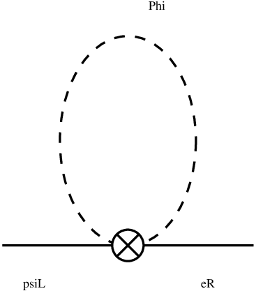
We should check whether the radiative correction induced by exchange of (Fig. 7) violates Koide’s mass formula or not. With the reference potential eq. (106), we consider the limit and consistently with the assumed hierarchy of the parameters. Physical modes of decouple in the former limit. Thus, we consider only and . One may determine the scalar mass eigenstates explicitly and find
| (114) |
Since it has a form , Koide’s formula will not be affected. This result may be more non–trivial than one might think at a first glance, since the diagram in Fig. 7 corresponds to incorporating the class of (infinite number of) 1–loop diagrams shown in Fig. 2. As a cross check, we also computed the coefficient of through renormalization of the operator in the symmetric phase ().
There are only three physical modes of which gain masses of order ; these are which are proportional to , and . The first mode gives the correction eq. (114), while the contributions of the second and third modes cancel. Other modes have masses suppressed by , so that their contributions to the loop diagram in Fig. 7 are suppressed.
In fact the same features apply to the general potential of and , if the parameters of the potential satisfies the hierarchical relations required to realize the vacuum configuration and (as discussed in Secs. 5 and 6). Namely, absence of radiative corrections to Koide’s formula induced by scalar exchanges can be shown in the limit (assuming that contributions from physical modes of decouple also in this case).
As we discussed in Sec. 2 with an example of underlying mechanism, it is assumed that operators other than , which contribute to the charged lepton masses at higher orders of , are absent (or strongly suppressed) at . Since these operators are non–invariant under , sizes of these operators are determined by the physics above the scale . Within the effective theory starting from this boundary condition, other operators are not induced radiatively at lower energy scales and the relation (41) is preserved (see also the discussion in Sec. 3).** * A simpler operator such as would be inappropriate for a candidate of , even though it gives the desired spectrum at tree level: This operator induces a mass matrix radiatively, upon contraction of and .
In the limit and , the root–mass–ratios of the charged leptons are given by , where . They are in reasonable agreement with the corresponding experimental values as we have seen in eqs. (60) and (61). It would be instructive to see how much corrections are induced to these values by the small parameters in the potential. For simplicity, let us compute corrections to the charged lepton spectrum , corresponding to the potential eq. (106) and the higher–dimensional operator eq. (109). The corrections read
| (115) | |||
| (116) | |||
| (117) |
As can be seen, the magnitude of the correction is larger for smaller mass eigenvalues, reflecting the nature of a hierarchical spectrum, as we discussed in Sec. 4. Comparing to eqs. (60) and (61), one finds constraints on typical orders of magnitude of the parameters as , , , , provided there is no correlation or fine tuning among these parameters, or with corrections. On the other hand, the overall normalization,
| (118) |
is subject to radiative corrections induced by electroweak gauge interaction (including QED), family gauge interaction and scalar exchanges, in addition to the and corrections.
We define the following quantity as a measure of the degree of violation of Koide’s mass relation:
| (119) |
This quantity vanishes if Koide’s relation is satisfied. With the reference potential and , the correction reads
| (120) | |||
| (121) |
Comparing to the present experimental value , we obtain constraints on typical sizes of the parameters more stringent than the previous ones: , , , .
It is easy to adjust the root–mass–ratios to be consistent with the current experimental values without violating Koide’s relation, as we discussed in Sec. 4. For instance, it is achieved by incorporating with into the potential.
8 Relevant Scales and Further Assumptions
Let us discuss the energy scales, , , , involved in the present model. It would be unnatural if there is a large hierarchy between and , or between and . As we speculated in Sec. 3, the scale of symmetry breaking, typically given by , may be at – TeV, such that the QED correction is cancelled within a scenario of unification of the electroweak and family symmetries. There are two indications that the cut–off scale and the symmetry breaking scale are not too far apart. One indication is the importance of the universality of the and gauge coupling constants eq. (20). This universality may be protected above the cut–off scale by embedding and in a simple group. If is very different from , however, the values of the two coupling constants at would become too different. Another indication consists in the relation (7), from which one derives
| (122) |
up to electroweak corrections, etc. is smaller than and is expected to be not very much smaller. Although it depends on the mechanism how the higher–dimensional operator is generated, if is not large (as one naively expects), hierarchy between and is mild. As for the scale , it is required to be smaller than in order not to alter the spectrum of the family gauge bosons. Numerically is required from the present constraint on Koide’s formula.
There are a few more assumptions implicit in the present model, which we have not discussed so far. We assume that the family gauge symmetry is broken spontaneously at a scale higher than . This is required to protect the symmetry breaking pattern eq. (33), which constrains the form of the radiative correction by the gauge bosons. To achieve this, we need additional fields or dynamics, such as an doublet scalar field whose VEV breaks . As yet, we have not succeeded to incorporate such a mechanism consistently into our model. Here, we simply assume that the breakdown of has occurred without affecting the properties of our model described above.
We also assume cancellation of gauge anomalies and decoupling of unwanted fermions. Namely, we assume cancellation of anomalies introduced by the couplings of fermions to family gauge bosons, at the scale where symmetry is unbroken. This means that we need fermions other than the SM fermions. Fermions other than the SM fermions are requisite in our model also because and are embedded into larger multiplets of . At lower energy scales, , all the additional fermions are assumed to aquire masses of order or larger, so that they decouple from the SM sector at and below the electroweak scale. Only the SM fermions remain at these scales. Presently we do not have a model which fully explains these features.
9 Lepton Flavor Violating Processes and Other Predictions
A most characteristic prediction of the present model is the existence of lepton–flavor violating processes induced by the family gauge interaction. In the scenario, in which the family gauge symmetry and weak gauge symmetry are unified at – TeV scale, the family gauge bosons have masses of the order of the unification scale.
As it is clear from eq. (3), flavor violating decays of a charged lepton with only charged leptons and/or photons in the final state, such as or , are forbidden. Flavor violating leptonic decays which involve neutrinos, such as , are allowed, but the present experimental sensitivities are very low. Presumably, the most sensitive process is , although we need to make assumptions on the quark sector. For instance, assuming that the down–type quarks are in the same representation of as the charged leptons, and that the mass matrices of the charged leptons and down–type quarks are simultaneously diagonalized in an appropriate basis, this process is induced by an effective 4–Fermi interaction connecting the first and second generations:
| (123) |
We find
| (124) |
Comparing to the present experimental bound [2], we obtain a limit TeV. Naively this limit may already be marginally in conflict with the estimated unification scale in the above scenario. We should note, however, that this depends rather heavily on our assumptions on the quark sector. In the case that there exist additional factors in the quark sector which suppress the decay width by a few orders of magnitude, we may expect a signal for not far beyond the present experimental reach. Similarly the process may also be observable in the future.
Another interesting observation, although it is much more model dependent, is the following. In order to stabilize Koide’s formula, in our model, it is necessary to suppress non–invariant operators in the potential of . This indicates that includes physical modes which are much lighter than – TeV. In particular, the lightest one, being singlet under the SM gauge group, may decay into leptons through the family gauge interaction or the operator with a significant branching ratio. Hence, if this lightest scalar boson happens to be produced at the LHC, an excess in multi-lepton final states may be observed.
10 Summary and Discussion
In this paper, we propose a model of charged lepton sector, in the context of an EFT valid below the cut–off scale , which predicts a charged lepton spectrum consistently with the experimental values. In particular, we implement specific mechanisms into the model, such that the spectrum satisfies Koide’s mass formula within the present experimental accuracy. In this model radiative corrections as well as other corrections to Koide’s formula are kept under control, and this feature primarily differentiates the present model from the other models in the literature which predict Koide’s formula. By studying within EFT, we circumvent many problems, at the price of introducing the cut–off scale at – TeV scale, while non–trivial relations between family symmetries and observed charged lepton spectrum can still be investigated.
In our model, we adopt a mechanism, through which the charged lepton mass matrix becomes proportional to the square of the VEV of a scalar field [10]. On the basis of this mechanism, we incorporate two new mechanisms in the model which are worth emphasizing:
- (i)
The radiative correction to Koide’s formula induced by family gauge interaction has the same form as the QED correction with opposite sign. This form is determined by the symmetry breaking pattern eq. (33) and the representations of and . Within a unification scenario, cancellation of the QED correction can take place.
- (ii)
A charged lepton spectrum, which has a hierarchical structure and approximates the experimental values, follows from a simple potential , under the condition that Koide’s formula is protected.
Existence of such simple mechanisms may indicate relevance of family gauge symmetry in relation to the charged lepton spectrum.
Our model is constructed as an effective theory valid below the cut–off scale respecting this symmetry. We introduce scalar fields , and as multiplets of , in which is embedded. It is assumed that is spontaneously broken to below the scale . We minimize the potential of the scalar fields and determine its classical vacuum. The charged lepton masses are related to the VEVs of the scalar fields at scale , ; at this scale radiative corrections to the VEVs essentially vanish within the effective theory. Then, the mass matrix of the charged leptons are given in terms of the VEVs, such that Koide’s mass formula is stabilized, and that the spectrum agrees with the experimental values. This is achieved formally without fine tuning of parameters in the model, except for (a) the tuning required for stabilization of the electroweak scale , and (b) the tuning required for the cancellation of the QED correction, that is, realizing at relevant scales. We argue that the latter tuning can be replaced by a tuning of the unification scale, within a scenario in which family gauge symmetry and weak gauge symmetry are unified at – TeV scale.
In addition our model may contain following fine tuning. We were unable to explore the parameter space of the –invariant potential sufficiently, due to technical complexity. It may be the case that certain fine tuning is necessary to realize the configuration eqs. (6)–(98) as a classical vacuum.
Evidently the present model is incomplete, since it is restricted to the charged lepton sector. The model should be implemented in a larger framework which incorporates at least the following aspects missing in the present model: (i) Including the quarks and explaining the masses and mixings of the quarks and neutrinos; (ii) Cancellation of anomalies introduced by the couplings of fermions to family gauge bosons; (iii) Unification of and gauge symmetries at – TeV scale. Possibly these problems are solved simultaneously in some model, and one anticipates that such a model would necessarily contain a large number of new particles, for the following reasons: (a) all the particles are embedded into multiplets of large groups, especially if one also requires to unify hypercharge and color gauge groups together with and ; (b) additional fermions are necessary to cancel anomalies; and (c) scalar fields would be necessary to give masses of order to fermions (apart from the SM fermions) through their VEVs [19].
Although our model predicts a realistic lepton spectrum, in fact many of the questions are simply reassigned to physics above the cut–off scale and remain unanswered: While we replaced the conditions on the lepton spectrum by the boundary conditions of the effective potential, we do not address which dynamics leads to these boundary conditions. (Only a speculation is given.) We may nevertheless state that not only did we circumvent fine tuning but also the problems actually simplified. The required boundary conditions are certain hierarchical structure among the couplings of the effective potential. These conditions would be simpler to realize than, for instance, to realize Koide’s relation among the lepton Yukawa couplings with accuracy a priori.
Phenomenologically our model predicts existence of lepton violating processes at – TeV scale, assuming the unification scenario at this scale. The processes and are expected to be sensitive to the predictions of our model, although we need additional assumptions on the quark sector. Stability of Koide’s formula indicates existence of light modes in , and the lightest mode may decay into leptons with a significant branching ratio; they may generate an interesting signal at the LHC.
It is unlikely that the present model describes Nature correctly to the details, since we can easily construct variants of the present model with similar complexity. Overall, the present model is rather complicated, and the source of complexity is conspiracy to realize Koide’s formula with a high accuracy. Hence, we place more emphasis on the major mechanisms incorporated in the model, which look appealing and may reflect physics that governs the spectrum of the charged leptons.
Acknowledgements
The author is grateful to K. Tobe for discussion. This work is supported in part by Grant-in-Aid for scientific research No. 17540228 from MEXT, Japan.
Appendices
Appendix A Generators of
Appendix B Decomposition of under
, which is in the of , decomposes into under . Explicitly they can be constructed as follows:
| (155) |
| (159) |
| (160) | |||
| (161) | |||
| (162) |
When , the corresponding VEVs of , and are given, respectively, by
| (163) | |||
| (164) | |||
| (165) |
Appendix C Properties of
C.1 Maximizing

We impose the conditions
| (166) |
If we maximize under these conditions,
all ’s can be made real simultaneously
by a common phase rotation.
Namely, there exists a phase such that
for all .
Proof:
Let
| (167) |
Then ’s satisfy
| (168) |
These equations represent a nonagon with a fixed length of circumference in the complex plane. is maximized when the nonagon collapses to a line, where all ’s are parallel to one another and antiparallel to in the complex plane with
| (169) |
See Fig. 8.
C.2 Variation of at
The variation of , defined by eq. (53),
is positive semi–definite at under
transformation.
Namely,
if with
,
.
Proof:
Let
| (170) |
Then, noting
| (171) |
satisfies the same relation:
| (172) |
Since ’s are real, ’s are also real. According to Sec. 4, is a configuration which minimizes under the condition and . Therefore, . Since and are connected by a transformation, . It follows .
Due to this property, is minimized at and under the constraint and .
C.3 transformations of and
transformation of is defined by
| (173) |
where . Equivalently,
| (174) |
with
| (175) |
Similarly transformation of is defined by
| (176) |
or
| (177) | |||
| (178) | |||
| (179) |
transformations of other fields are the same as those of the SM.
For example, defined by eq. (69) is –invariant. An example of non–invariant operator is
| (180) |
with
| (181) |
C.4 Stability of at
When is invariant under and ,
its first derivative vanishes
at .
Proof:
| (182) |
Due to the residual symmetry of the VEV , the differential coefficients evaluated at take following forms:
| (183) | |||
| (184) |
where ’s are constants. Substituting to eq. (182), we have
| (185) |
where we used .
An arbitrary infinitesimal variation of , which is symmetric and unitary, can be parametrized by
| (186) |
with
neglecting terms. An explicit calculation shows that, for a variation , , , and depend only on for . (In this proof, no sum is taken over in without explicit summation symbol .) Hence,
| (192) |
On the other hand, applying transformation eq. (176) to , one finds that is –even, whereas all the coefficients of in are –odd. This means, if is –invariant,
| (193) |
so that the first derivative vanishes,
.
Appendix D , and Their Potential
D.1 Minimum of
We show that , given by eqs. (84) and (85), is minimized at the configuration eq. (86) in the limit .
It is known [18] that, for , is minimized at
| (194) |
where is an arbitrary 3–by–3 unitary matrix. Let
We assume that all ’s are different. Substituting eqs. (194),(D.1) to , it is expressed as
| (199) |
is unitary. Define
| (200) |
Then , since . Hence, is minimized when . This means and , where is an arbitrary diagonal unitary matrix defined in eq. (3); it can be absorbed into a redefinition of as .
D.2 Relation between and
is in the (, ) under , where stands for the second-rank antisymmetric representation of . is defined to be unitary. Thus,
| (201) |
The indices take values .
An orthonormal basis of –by– matrices is denoted by with the normalization condition
| (202) |
In particular, the first 9 bases are taken as
We may identify embedded in as follows.
| (206) | |||
| (210) | |||
| (211) |
D.3 A vacuum of the –invariant potential
We analyze a vacuum configuration of the –invariant potential given by eq. (99). We restrict our analysis to the case and consider only for and arbitrary , while all other are set equal to zero. In this restricted parameter space spanned by , we examine if the configuration given by eqs. (6)–(98) can minimize . We assume that the charge vanishes,
| (212) |
only in the sector for which . This is not a strong condition: Except when and satisfy specific relations, this condition is met.
We have checked the following two properties. (I) At each point of the parameter space, the first derivative of vanishes at the configuration eqs. (6)–(98), if
| (213) |
(II) The configuration eqs. (6)–(98) minimizes , if the condition (213) is satisfied and at each point in a hypersurface in the parameter space; the hypersurface is defined by the condition if and for all , while if or for any . These two properties (I)(II) ensure that, of each point in , there exists a neighborhood, which has a non–zero volume, and in which is minimized by the configuration in question. Namely, there exists a finite volume (non–zero measure) in the parameter space (at least) in a neighborhood of , in which the desired configuration becomes a vacuum.
The above properties (I)(II) are verified in the following manner. It suffices to show that all for can be brought to zero simultaneously at the configuration eqs. (6)–(98) by appropriately adjusting components of except for . In fact, in this case, as well as its first derivative vanish at any point of the parameter space. Thus, property (I) follows. Since in , the property (II) follows as well. We have checked numerically that all can be brought to zero at the configuration eqs. (6)–(98) by explicitly constructing the corresponding for a given value of . This turned out to be possible (at least) if the condition (213) is met, since there are quite large degrees of freedom in the choice of . (If is too large, it conflicts the unitarity condition of .)
References
- [1] Y. Koide, Nuovo Cim. A 70 (1982) 411 [Erratum-ibid. A 73 (1983) 327].
- [2] C. Amsler et al. [Particle Data Group], Phys. Lett. B 667 (2008) 1.
- [3] R. Foot, arXiv:hep-ph/9402242.
- [4] Y. Koide, Phys. Rev. D 28 (1983) 252; S. Esposito and P. Santorelli, Mod. Phys. Lett. A 10 (1995) 3077.
- [5] For a review, see Y. Koide, arXiv:hep-ph/0506247.
- [6] N. Li and B. Q. Ma, Phys. Rev. D 73 (2006) 013009.
- [7] Z. z. Xing and H. Zhang, Phys. Lett. B 635 (2006) 107.
- [8] E. Ma, Phys. Lett. B 649 (2007) 287.
- [9] For recent works, see G. Rosen, Mod. Phys. Lett. A 22 (2007) 283; Y. Koide, Phys. Lett. B 665 (2008) 227; J. Phys. G 35 (2008) 125004; Phys. Rev. D 78 (2008) 093006; arXiv:0811.3470 [hep-ph]; N. Haba and Y. Koide, Phys. Lett. B 659 (2008) 260; JHEP 0806 (2008) 023, and references therein.
- [10] Y. Koide, Mod. Phys. Lett. A 5 (1990) 2319.
- [11] Y. Sumino, Phys. Lett. B 671, 477 (2009).
- [12] Y. Koide and M. Tanimoto, Z. Phys. C 72, 333 (1996).
- [13]
Y. Koide and H. Fusaoka,
Z. Phys. C 71 (1996) 459;
Y. Koide and M. Tanimoto,
Z. Phys. C 72 (1996) 333.
See also [5] and references therein. - [14] Y. Koide, Phys. Rev. D 73, 057901 (2006).
- [15] There are a large number of papers on the fermion flavor structure based on or family symmetry. See, for instance, Z. G. Berezhiani and M. Y. Khlopov, Sov. J. Nucl. Phys. 51 (1990) 739; S. F. King, JHEP 0508 (2005) 105; I. de Medeiros Varzielas and G. G. Ross, Nucl. Phys. B 733 (2006) 31; T. Appelquist, Y. Bai and M. Piai, Phys. Rev. D 74 (2006) 076001; S. Antusch, S. F. King and M. Malinsky, JHEP 0806 (2008) 068, and references therein.
- [16] O. M. Del Cima, D. H. T. Franco and O. Piguet, Nucl. Phys. B 551 (1999) 813.
- [17] Earlier works are L. Dolan and R. Jackiw, Phys. Rev. D 9, 2904 (1974); N. K. Nielsen, Nucl. Phys. B 101, 173 (1975); R. Fukuda and T. Kugo, Phys. Rev. D 13, 3469 (1976). See also [16] and references therein.
- [18] L. F. Li, Phys. Rev. D 9 (1974) 1723.
- [19] Y. Sumino, in preparation.