Degree distributions of the visibility graphs mapped from fractional Brownian motions and multifractal random walks
Abstract
The dynamics of a complex system is usually recorded in the form of time series, which can be studied through its visibility graph from a complex network perspective. We investigate the visibility graphs extracted from fractional Brownian motions and multifractal random walks, and find that the degree distributions exhibit power-law behaviors, in which the power-law exponent is a linear function of the Hurst index of the time series. We also find that the degree distribution of the visibility graph is mainly determined by the temporal correlation of the original time series with minor influence from the possible multifractal nature. As an example, we study the visibility graphs constructed from two Chinese stock market indexes and unveil that the degree distributions have power-law tails, where the tail exponents of the visibility graphs and the Hurst indexes of the indexes are close to the linear relationship.
Keywords:
Visibility graph; complex networks; power-law distribution; fractional Brownian motion; multifractal random walkPACS
89.75.Hc,05.40.-a, 05.45.Df, 05.45.Tp1 Introduction
Complex systems are ubiquitous in natural and social sciences, where the constituents interact with one another and form a complex network. In recent years, complex network theory has stimulated explosive interests in the study of social, informational, technological, and biological systems, resulting in a deeper understanding of complex systems [1, 2, 3, 4]. However, for many complex systems, it is hard to obtain detailed information of interacting constituents and their ties, which makes the underlying network invisible. Instead, we are able to observe and record a time series generated by the system. For such cases, time series analysis becomes a crucial way to unveil the dynamics of complex systems. There are also some efforts to map time series into graphs to study time series from the network perspective, which amounts to investigating the dynamics from the associated network topology.
For a pseudoperiodic time series, one can partition it into disjoint cycles according to the local minima or maxima, and each cycle is considered a basic node of a network, in which two nodes are deemed connected if the phase space distance or the correlation coefficient between the corresponding cycles is less than a predetermined threshold [5]. We note that a weighted network can also be constructed if the phase space distance or the correlation coefficient is treated as the weight of a link. This method for pseudoperiodic time series can also be generalized to other time series, where a node is defined by a sub-series of a fixed length as the counterpart of a cycle, which has been applied to stock prices [6].
Another method for network construction from time series is based on the fluctuation patterns [7, 8]. In this approach, each data point is encoded as a symbol R, r, D, or d, corresponding to big rise, small rise, big drop and small drop, respectively. The time series is then transformed into a symbol sequence. Defining a fluctuation pattern as an -tuple consist of a string of symbols, the symbol sequence can be further mapped into a sequence of non-overlapping -tuples. The -tuples are treated as nodes of the constructed network. Therefore, the number of nodes does not exceed . Two nodes are connected if the associated -tuples appear one after the other in the pattern sequence. Furthermore, the edge weight between two nodes can be defined as the occurrence number of two successive patterns in the sequence. This approach has been applied to study the price trajectory of Hang Seng index [7, 8].
A third method is to convert time series into visibility graphs based on the visibility of nodes [9]. For simplicity, consider an evenly sampled time series . Each data point of the time series is encoded into a node of the visibility graph. Two arbitrary data points and have visibility if any other data point located between them fulfills
| (1) |
Two visible nodes become connected in the associated graph. An example of a time series containing 16 data points and the associated visibility graph derived from the visibility algorithm is illustrated in Fig. 1. By definition, any visibility graph extracted from a time series is always connected since each node sees at least its nearest neighbor(s) and the degree of any node with is not less than 2. In addition, a periodic time series converts into a regular graphs, whose degree distribution is formed by a finite number of peaks related to the series period, while random time series lead to irregular random graphs [9]. It is also found that visibility graph is invariant under affine transformations of the series data since the visibility criterion is invariant under rescaling of both horizontal and vertical axes, and under horizontal and vertical translations [9].
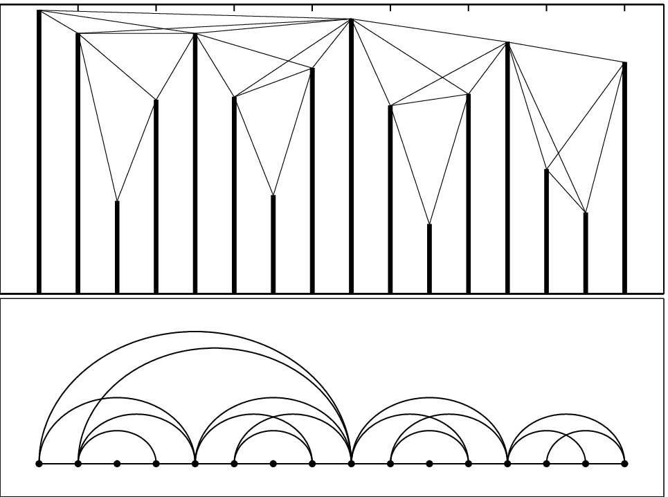
Degree distribution is one of the most important characteristic properties of complex networks [10]. The degree distribution of the visibility graphs of several specific examples of time series have been investigated [9]. For a random time series extracted from an uniform distribution in , the degree distribution of the visibility graph has an exponential tail . Alternatively, the visibility graphs of Brownian motions and Conway series are scale-free, characterized by a power-law tail in the degree distribution:
| (2) |
where for Brownian motions and for Conway series. It is also conjectured that the temporal correlation of the time series (characterized by its Hurst index ) might have influence on the degree distribution of its visibility graph [9]. In this work, we test this projection based on extensive numerical simulations. Specifically, fractional Brownian motions (FBMs) [11] and multifractal random walks (MRWs) [12] are synthesized to investigate the influence of autocorrelation and multifractality on the degree distribution.
2 Numerical analysis
2.1 Generating FBMs and MRWs
There are many different algorithms for the generation of fractional Brownian motions [13] and we adopt a wavelet-based algorithm to simulate FBMs [14]. On the other hand, a multifractal random walk can be generated by the cumulative summation of the increments
| (3) |
where is a fractional Gaussian noise with Hurst index , is a correlated Gaussian noise, and they are independent [12]. We use the detrended fluctuation analysis [15, 16] to verify if the resultant Hurst index of the generated signals is identical to the input value of in the algorithms. For each , we generate 10 realizations and calculate the mean Hurst index . The results are presented in Fig. 2. The top panel of Fig. 2 shows that the estimated Hurst indexes of the synthesized FBMs are very close to the input value with minor deviation for small . For MRWs, we find that when and a systematic deviation when . In addition, we have confirmed that the generated MRW signals possess multifractal nature.


2.2 Numerical results
We have investigated FBMs with the input Hurst index ranging from 0.1 to 0.9 in the spacing of 0.1. For each , we repeat the simulation 100 times and each simulation gives a FBM signal with the size . For each FBM signal, a visibility graph is constructed and its empirical degree distribution is determined. We find that the 100 distributions almost collapse onto a single curve. This enables we to put all the data of the 100 graphs to construct the empirical degree distribution to gain better statistics. Three typical empirical degree distributions of the visibility graphs converted from FBM series with different Hurst indexes are depicted in Fig. 3(a). Nice power-law behaviors are observed in the distributions, followed by faster relaxation. We note that the visibility graphs of other FBMs also exhibit power-law tails in the degree distribution.


The situation is very similar for the MRW case. We have simulated MRW signals of size with different input Hurst index ranging from 0.05 to 0.95 with an increment of 0.05. For each , 100 MRW signals are simulated and then converted to 100 visibility graphs. Three typical empirical degree distributions of the visibility graphs are depicted in Fig. 3(b) for different Hurst indexes (not ). All the distributions exhibits nice power laws with faster decay for large degrees.
The power-law exponents of the distributions are calculated in the scaling ranges. Figure 4 shows the dependence of the power-law exponents on the Hurst indexes . Both curves show a nice linear relationship:
| (4) |
A least-squares regression gives and for FBMs and and for MRWs. We find that the multifractal nature of the MRWs has minor influence on the degree distributions of the visibility graphs.


We note that, the linear relationship between the tail exponent and the Hurst index was also found for fractional Brownian motions independently [17].
3 Applications to financial data
In this section, we apply the visibility graph method to financial data. Specifically, two indices of the Chinese stock market are considered. The organized stock market in mainland China is composed of two stock exchanges, the Shanghai Stock Exchange (SHZE) and the Shenzhen Stock Exchange (SZSE). Shanghai Stock Exchange Composite index (SHCI) and Shenzhen Stock Exchange Component index (SZCI) are the representative indices for the two stock exchange, respectively. Our analysis is based on the 1-min data of the two indices. The time series spans from 2 January 2001 to 28 December 2007 for the SHCI and from 4 January 2002 to 28 December 2007 for the SZCI. The temporal evolution of the price trajectories of the two indices are illustrated in Fig. 5. According to Fig. 5, the Chinese stock market was in a bearish phase from 2001 to 2005, which is known as an antibubble [18], and then the market reversed and produced a very marked bubble which burst at the end of 2007. In order to test if the market phase has impact on the results, we partition each time series into two sub-series delimited on 31 December 2005, corresponding to the bear period and the bull period, respectively.

For each index, we obtain three visibility graphs corresponding to the bear period, the bull period, and the whole time period. The empirical degree distributions of the three visibility graphs are determined. Fig. 6 shows the results of SHCI. We note that the results for the SZCI are very similar.

We observe that all the distributions have heavy tails and the degree distribution in the bear period can be well modeled by a power law (2) in the right part. The rapid decay does not mean that the power law is truncated but rather reflects the fluctuations at finite size [19]. The tail exponent is estimated to be . For the case of the bull period, there is a hump in the tail. This phenomenon is more evident for the whole period, which is caused by the fact that there are more points in the bull period that can see more previous points (large degrees). There are two power laws in the degree distributions for the whole time period case, illustrated by two parallel dashed lines in Fig. 6. The estimates of the tail exponents for SHCI and SZCI are listed in Table 1.
| SHCI | SZCI | ||||||
|---|---|---|---|---|---|---|---|
| Bear | Bull | Whole | Bear | Bull | Whole | ||
| 0.52 | 0.50 | 0.51 | 0.54 | 0.51 | 0.52 | ||
| 1.95 | 1.88 | 2.00 | 1.92 | 1.67 | 1.72 | ||
| 1.85 | 1.92 | 1.87 | 1.82 | 1.88 | 1.85 | ||
| 0.05 | -0.02 | 0.06 | 0.05 | -0.11 | -0.07 | ||
In order to compare the empirical results with the numerical results in Section 2, we determine the Hurst indexes of the log returns for each index by applying the detrended fluctuation analysis. The results are listed in Table 1. One finds that the Hurst indexes are undistinguishable from . The multifractal detrended fluctuation analysis [20] confirms that all the time series possess multifractal nature. Therefore, the tail exponents can be “predicted” according to the linear relationship . The predicted tail exponents are also presented in Table 1. It is found that the discrepancy between and is not large, which is quantified by the relative difference shown in Table 1. Fig. 7 further illustrate this point by the scatter plot of the six data points . These data points are very close to the dot-dashed line , showing that the empirical results are consistent with the numerical analysis in Section 2.

4 Conclusion
In summary, we have studied the degree distributions of visibility graphs extracted from fractional Brownian motions and multifractal random walks. We found that the degree distributions exhibit power-law behaviors, in which the power-law exponent is a linear function of the Hurst index inherited in the time series. In addition, the degree distribution of the visibility graph is mainly determined by the temporal correlation of the corresponding time series, and contains minor information about the multifractal nature of the time series. The linear relation (4) provide a possible tools for the determination of of a time series from its visibility graph [9]. However, cations should be taken since the increments distribution of the time series might also have impact on the degree distribution.
Acknowledgments:
This work was partly supported by the National Natural Science Foundation of China (70501011), the Program for New Century Excellent Talents in University (NCET-07-0288), the Shanghai Educational Development Foundation (2008SG29), and the China Scholarship Council (2008674001).
References
- [1] R. Albert, A.-L. Barabási, Statistical mechanics of complex networks, Rev. Mod. Phys. 74 (2002) 47–97. doi:10.1103/RevModPhys.74.47.
- [2] M. E. J. Newman, The structure and function of complex networks, SIAM Rev. 45 (2) (2003) 167–256. doi:10.1137/S003614450342480.
- [3] S. N. Dorogovtsev, J. F. F. Mendes, Evolution of Networks: From Biological Nets to the Internet and the WWW, Oxford University Press, Oxford, 2003.
- [4] S. Boccaletti, V. Latora, Y. Moreno, M. Chavez, D.-U. Hwang, Complex networks: Structure and dynamics, Phys. Rep. 424 (2006) 175–308. doi:10.1016/j.physrep.2005.10.009.
- [5] J. Zhang, M. Small, Complex network from pseudoperiodic time series: Topology versus dynamics, Phys. Rev. Lett. 96 (2006) 238701. doi:10.1103/PhysRevLett.96.238701.
- [6] Y. Yang, H.-J. Yang, Complex network-based time series analysis, Physica A 387 (2008) 1381–1386. doi:10.1016/j.physa.2007.10.055.
- [7] P. Li, B.-H. Wang, An approach to Hang Seng Index in Hong Kong stock market based on network topological statistics, Chinese Science Bulletin 51 (2006) 624–629. doi:10.1007/s11434-006-0624-4.
- [8] P. Li, B.-H. Wang, Extracting hidden fluctuation patterns of Hang Seng stock index from network topologies, Physica A 378 (2007) 519–526. doi:10.1016/j.physa.2006.10.089.
- [9] L. Lacasa, B. Luque, F. Ballesteros, J. Luque, J. C. Nuño, From time series to complex networks: The visibility graph, Proc. Natl. Acad. Sci. U.S.A. 105 (2008) 4972–4975. doi:10.1073/pnas.0709247105.
- [10] A.-L. Barabási, R. Albert, Emergence of scaling in random networks, Science 286 (1999) 509–512. doi:10.1126/science.286.5439.509.
- [11] B. B. Mandelbrot, J. W. Van Ness, Fractional Brownian motions, fractional noises and applications, SIAM Rev. 10 (1968) 422–437. doi:10.1137/1010093.
- [12] E. Bacry, J. Delour, J.-F. Muzy, Multifractal random walk, Phys. Rev. E 64 (2001) 026103. doi:10.1103/PhysRevE.64.026103.
- [13] J.-M. Bardet, G. Lang, G. Oppenheim, A. Philippe, S. Stoev, M. S. Taqqu, Generators of long-range dependence processes: A survey, in: P. Doukhan, G. Oppenheim, M. Taqqu (Eds.), Theory and Applications of Long-Range Dependence, Birkhauser, New York, 2003, pp. 579–623.
- [14] P. Abry, F. Sellan, The wavelet-based synthesis for the fractional Brownian motion proposed by F. Sellan and Y. Meyer: Remarks and fast implementation, Appl. Comp. Harmonic Anal. 3 (1996) 377–383. doi:10.1006/acha.1996.0030.
- [15] C.-K. Peng, S. V. Buldyrev, S. Havlin, M. Simons, H. E. Stanley, A. L. Goldberger, Mosaic organization of DNA nucleotides, Phys. Rev. E 49 (1994) 1685–1689. doi:10.1103/PhysRevE.49.1685.
- [16] J. W. Kantelhardt, E. Koscielny-Bunde, H. H. A. Rego, S. Havlin, A. Bunde, Detecting long-range correlations with detrended fluctuation analysis, Physica A 295 (2001) 441–454. doi:10.1016/S0378-4371(01)00144-3.
- [17] L. Lacasa, B. Luque, J. Luque, J. C. Nuño, The visibility graph: A new method for estimating the Hurst exponent of fractional Brownian motion, arXiv: 0901.0888 (2009).
- [18] W.-X. Zhou, D. Sornette, Antibubble and prediction of China’s stock market and real-estate, Physica A 337 (2004) 243–268. doi:10.1016/j.physa.2004.01.051.
- [19] T. Maillart, D. Sornette, S. Spaeth, G. von Krogh, Empirical tests of Zipf’s law mechanism in open source Linux distribution, Phys. Rev. Lett. 101 (2008) 218701. doi:10.1103/PhysRevLett.101.218701.
- [20] J. W. Kantelhardt, S. A. Zschiegner, E. Koscielny-Bunde, S. Havlin, A. Bunde, H. E. Stanley, Multifractal detrended fluctuation analysis of nonstationary time series, Physica A 316 (2002) 87–114. doi:10.1016/S0378-4371(02)01383-3.