Sciences \professorT. Giamarchi \departmentshortDPMC \cityofbirthCaracas Venezuela \thesisnumber0001 \departmentDépartement de Physique la Matière condensée \universityUniversité de Genève \yeargrad2008 \degreePhilosophiæDoctor (PhD) \degreedate30/6/2008 \memberAChristophe BerthodCodirecteur de thèseUniversité de Genève \memberBDirk van der MarelProfesseurUniversité de Genève \memberCAntoine GeorgesProfesseurÉcole Polytechnique \approvaldate12 Septembre 2008 \deanJean-Marc TRISCONE
Study of the Hall effect in two different strongly correlated fermion systems
Abstract
Put your abstract or summary here, if your university requires it.
\fancyendSimplemente a mi familia
Ce travail a été consacré a l’étude de l’effet Hall dans deux systèmes différents de fermions fortement correlés: un système constitué de liquides de Luttinger faiblement couplés et dans un réseau triangulaire bidimensionnel. Dans le but d’avoir les outils nécessaires pour attaquer ces problèmes, on a entrepris une révision des propriétés principales des systèmes avec des intéractions fortes, en nous concentrant dans les systèmes à deux dimension et à basse dimensionnalité (1D et quasi 1D). Etant donné que l’effet Hall est avant tout un phenonème de transport, on a étudié les formalismes existants dans la littérature pour traiter les propriétés de transport dans les systèmes fortement correlés, et nous avons consacré tout un chapitre au traitement spécifique de l’effet Hall.
Donc en un premier temps nous avons étudié le modèle des liquides de Luttinger faiblement couplés. L’étude de l’effet Hall dans un système quasi 1D a été partiellement motivée par les résultats expérimentaux obtenus sur des conducteurs organiques quasi 1D. Ce travail était basé sur l’application du formalisme de matrice mémoire pour obtenir la constante de Hall () dans des chaines a moitié remplis faiblement couplées, incluant la diffusion umklapp. La géométrie du modèle a été choisie pour avoir le courant circulant le long des chaines 1D. On a calculé la dépendance en temperature et fréquence de en tenant compte des intéractions particule-particule et particule-réseau (processus umklapp). On a obtenu un coefficient de Hall constitué d’abbord par un terme d’éléctrons libres (valeur de bande ) plus un terme de corection avec une dépendance en temperature (fréquence) donné par une loi de puissance, due à la présence de la diffusion umklapp. Ces lois des puissance sont des signatures du comportement des liquides Luttinger, où les exposants dépendent des paramètres d’interactions. Le coefficient de Hall a aussi été calculé dans le système sans intéraction particule-particule, condisuant à une dépendance logarithmique en (où ), en accord avec la limite d’interaction nulle de la loi de puissance. Etant donné que les conducteurs organiques quasi 1D sont en même temps des systèmes à moitié remplis et au quart remplis, nos résultats théoriques ne sont pas directement applicables aux messures d’effect Hall existantes, mais ils nous ont permis d’arriver a des conclusions intérésantes. En premier lieu, la façon appropiée d’analyzer les messures d’effet Hall realisées dans ces sytèmes quasi 1D (dans la même geométrie du modèle), est de fitter les deviations de la valeur de bande \fancyend
Chapter 1 Introduction
It is likely that Edwing Herbert Hall was not aware of the enormous impact that his experimental results would have when he measured the Hall voltage for the first time in 1879. Not only because the Hall effect has allowed to determine the sign and density of the charge carriers of many materials, but also because it lead to a whole new field of research on the nature of the particles responsible for the electrical current in any system.
Nowadays, the Hall resistivity has become a common tool when studying the transport properties of any new material. However real experiments have shown that this phenomenon cannot always be interpreted in terms of the density of charge carriers and thus, has to be interpreted in a different way. Compounds can have strong interactions affecting the transport properties. Such strongly interacting systems are now at the heart of research in condensed matter physics and the understanding of the effect of these interactions is crucial for the description of these materials.
In this work we undertake the challenging task of studying the Hall effect in two different systems taking into account interactions. This requires the study of the existing methods for treating strongly interacting systems and their application to the Hall effect. We have chosen two model systems which are similar to real compounds where the measured Hall effect cannot be readily explained. The work presented here is entirely theoretical but some applications to real experiments are discussed. The plan of the work is presented in what follows.
We begin this manuscript with a description of the standard theoretical models used to describe two-dimensional and low-dimensional fermions systems with strong correlations. In particular, we review the main properties of the two-dimensional square lattice and the 2D triangular lattice, and then those of one-dimensional and quasi one-dimensional systems.
The second chapter is devoted to the transport phenomena in systems with strong interactions. For this we explain the linear response theory and the Kubo formulas. Such formulas are necessary for the understanding of the memory function formalism developed afterwards. We end this chapter with an application of the previously mentioned theories in the calculation of transport properties in low-dimensional systems.
The third chapter is completely dedicated to the Hall effect. We begin with the explanation of the classical Hall effect. Next, we obtain an expression for the Hall resistivity at infinite frequency and finally, we use the memory formalism to include interactions in the expression of the Hall resistivity.
Our first theoretical contribution is presented in the fourth chapter. The Hall effect is investigated in a quasi one-dimensional system made of weakly coupled 1D chains. For this we begin with a review on quasi 1D organic conductors, specifically in Bechgaard and Fabre salts, where various Hall measurements have been accomplished. We explain the model and methods used to calculate the Hall constant. We then present the results and discuss their range of validity and application to real experiments.
In the fifth chapter we present our second theoretical work. In this case we consider the two-dimensional triangular lattice as our model system. We start with the description of the sodium cobalt oxide, a compound with a triangular lattice structure, where the Hall effect have been investigated recently. As before, we introduce the model and methods used to calculate the Hall constant. We present the results obtained and discuss their range of validity and application to the previously mentioned experiments.
We close this manuscript with some general conclusions from the two theoretical works presented and perspectives for future works. Some appendices are presented at the end.
Strongly correlated systems
In condensed matter physics, understanding the effects of interactions in real materials, has occupied theoretical and experimental physicists for more than fifty years now. Depending on the strength of interactions the convenient approach to be implemented can be completely different. For example, if interactions are very weak, like in metals, the free-electron model works well to describe most of the physical properties. The dimensionality also plays a crucial role in this choice. In general, high-dimensional interacting systems are well described by the Fermi Liquid theory, where electrons are dressed by the density fluctuations around them, forming individual objects called quasiparticles, as formulated by Landau and others [1, 2, 3]. The fraction of the electrons that remain in this quasiparticle state is called the residue , and gives the amplitude of the discontinuity in the occupation factor . The big result of the Fermi liquid theory is that the properties of the interacting system remain essentially the same of the free fermionic particles.
In one dimension, on the contrary, the Fermi Liquid theory breaks down and is the Luttinger Liquid theory that describes the physics, even in systems with very strong interactions, as explained in Sec. One-dimensional case. Furthermore, Fermi Liquid theory is not always applicable in high-dimensions when one is working with strong interactions. The common characteristic of strongly correlated systems, where one finds materials as different as heavy fermions, high Tc superconductors, cobalt oxides and organic conductors, is a narrow band where fermions interact strongly on a scale of the order of electronvolts at short distances. In two-dimensional systems, for example, none of the previously mentioned theories is applicable when strong interactions are present. Then, basic models such as the Hubbard, -, Anderson and Kondo lattice models had to be implemented in an effort to understand the properties of these strongly correlated layered materials.
As we are interested in the study of the Hall effect in a quasi one-dimensional system and in a two-dimensional triangular lattice, we will devote this chapter to the description of the theoretical models used to describe these systems throughout this work. First, we will study the main properties of the two-dimensional Hubbard model, focusing on two geometries: the rectangular and the triangular lattice. Then, for the case of low-dimensional systems, we will make a short review on the Luttinger liquid theory and its extension to describe quasi one-dimensional systems.
The Hubbard model
The Hubbard model is one of the simplest models existing in literature [2] to describe the physics of interacting fermions on a lattice. Hubbard (1963) proposed an extension of the tight-binding model [2], where electrons hop from site to site with a matrix element , adding a term that provides a penalty for any atomic site occupied by more than one electron. This is depicted in Fig. 1.1. In terms of fermionic operators, the Hubbard Hamiltonian takes the following form [2]
| (1.1) |
where is the creation (annihilation) fermion operator, is the fermionic number operator and are nearest-neighboring sites. The first term in Eq. (1.1) represents the kinetic energy of the electrons and the second term correspond to the interaction between them. In addition, we include a chemical potential in order to adjust the number of electrons in the system.
There are extensions of the Hubbard model in which electron hopping beyond nearest-neighbors and electron-electron interaction at larger distances, are taken into account. We will not treat these models here because they are beyond the scope of this work, and we refer the reader to the literature for a complete description of these cases [2]. The Hubbard model was solved exactly in one dimension, by Lieb and Wu (1968) [4], as we will discuss it in the next section. For dimensions greater than one, many attempts have been undertaken to derive a phase diagram at zero temperature using random phase approximation (RPA) [2], mean field theory [5], numerical methods as the dynamical mean field theory (DMFT) [6], etc; but there are still many open questions and discrepancies between different approaches.
When working with the Hubbard model, there are two important energy scales to take into account: the on-site Coulomb interaction and the bandwidth . They determine the behavior of the system by the value of the ratio . If this ratio is small, the free-electron model can be used to describe most of the physical properties of the system. Simple metals like aluminium or sodium have . On the other hand if the ratio is large, then and electron correlations are dominant. This case is not fully understood but some of its properties are currently well characterized. We list some of them below.
The electron density ( being the number of electrons and the number of lattice sites) varies from to , due to Pauli principle. When there are two electrons in each site, they cannot move, and the system is an insulator. At half filling, when there is exactly one electron per site (), the ground state is antiferromagnetic (AF), i.e., neighboring spins pointing in opposite directions. Furthermore, if and there is one particle per site, the system is in an insulating state known as a Mott insulator [7, 8]. Possible phases of the Hubbard model are: the paramagnetic phase, the ferromagnetic phase, the charge-density wave phase (CDW) and the spin density wave phase (SPW) [2]. Each of these phases has particular properties which have been studied extensively in the last decades. Nevertheless a unique phase diagram for the Hubbard model for dimensions , is still lacking.
One important property of the Hubbard model at half-filling is the particle-hole symmetry, which means that the Hamiltonian in Eq. (1.1) is invariant under the electron-hole transformation: , where () creates (annihilates) a hole. This property is very peculiar to half-filled bi-partite lattices (lattices that can be decomposed into a disjoint union of two sublattices) and is not fulfilled, for example, on the triangular lattice (see Sec. The 2D triangular lattice).
An special limit of the Hubbard model that will be studied in Chapter. Hall effect on the strongly correlated 2D triangular lattice is called the atomic limit and corresponds to a system where the hopping amplitude is set to . In this case the system consist on isolated sites where particles cannot move from site to site. An exact solution can be found for the atomic limit of the Hubbard model (each site is considered individually), for any dimension (see Appendix. Self-energy and distribution function in the atomic limit). Another exactly solvable limit is the limit (tight-binding model), where the Hubbard Hamiltonian can be also completely diagonalized. The properties of the Hubbard model strongly depend on the type of the lattice and on the dimensionality. That is why we will focus here only on two geometries of the 2D Hubbard model: the square lattice and the triangular lattice. But, before entering into these two particular geometries, we will mention another variant of Hamiltonian (1.1) known as the - model [9].
The - model describes a system of interacting fermions on a lattice where the on-site interaction is considered infinite, in order to prohibit double occupancy, i.e., sites with . This constraint is implemented using the Gutzwiller projection operator . Applying this operator to Hamiltonian (1.1) one obtains “exchange term”, where the exchange term is given by , with the spin operator at site i. The exchange term represents an effective antiferromagnetic interaction between neighboring spins, which results from the virtual hopping of electrons into and out of doubly-occupied states, and has an amplitude . The - model has no exact solution either, but it is widely used in the study of fermionic systems with very strong interactions. We will not study the properties of the - model here because we are interested in the effect of interactions as a function of their strength, and for this the Hubbard model is the more accurate model to describe our two-dimensional systems. But it remains a good model to make comparisons at very strong interactions, as will be done in Chapter Hall effect on the strongly correlated 2D triangular lattice. We refer the reader to the literature for a complete review on the - model [10, 11].
The 2D square lattice
In this section we will study some general properties of the square lattice and definitions that will be useful in the rest of this work. Then, we will give the properties of the Hubbard model in this particular geometry. The two-dimensional square lattice has the structure shown in Fig. 1.1 which is invariant under translation (it has translational symmetry). The lattice is defined by two primitive vectors and , where is the intersite distance, called the lattice parameter. The real space lattice, often referred as direct lattice, can also be represented in momentum space. The latter is known as the reciprocal lattice and is formed by the set of vectors satisfying , with a vector of the direct lattice [12]. The two primitive reciprocal vectors are and . We will see, in a minute, how any vector on k-space is defined by and . Due to the periodicity of the lattice, it properties can be studied in a reduced zone or primitive cell of the reciprocal space defined by the Wigner-Seitz cell of the origin, which associates with each lattice point all of space which is closer to it than any other lattice point [5]. This is the Brillouin zone (see Fig. 1.2).
One important quantity that changes from one geometry to the other, is the dispersion relation or momentum energy of the particles. It also depends on the model used. Let us take the previously studied Hubbard model to describe the 2D square lattice. The dispersion relation is obtained by transforming the Hamiltonian to momentum space, using the Fourier transform of fermionic operators
| (1.2) |
where is the volume of the system. The inverse Fourier transform is thus given by . We will also need the Fourier transform of the number operator, which is
| (1.3) |
Then, Fourier transforming Hamiltonian (1.1) we obtain [2]
| (1.4) |
The coefficient of the first term in Eq. (1.4) (the kinetic energy term) gives the dispersion relation of the 2D square lattice. Thus, the dispersion relation is
| (1.5) |
where is the lattice parameter (, with nearest-neighboring sites). In Eq. (1.5) we supposed an isotropic square lattice. The components and of any vector in the reciprocal lattice are obtained from the primitive vectors and trough the relation: and , where and are integers. The dispersion relation determines the bandwidth () of the system, which is given by the range of energies between the maximum and minimum of . As can be seen from Eq. (1.5), the bandwidth of the 2D square lattice is equal to . The dispersion relation is often written with reference to the chemical potential, combining the 1st and 3rd terms on the right hand side of Eq. (1.4): .
The ground state of the non-interacting system ( in Hamiltonian (1.4)) is constructed by occupying all the energy-levels with two electrons with opposite spins, until reaching the total number of particles . The highest energy level is called the Fermi level and has an energy , with the Fermi momentum. This energy level allows to define the "Fermi surface", which is an important quantity when studying real materials (nowadays measured experimentally with different methods, such as angle resolved photoemission spectroscopy). The Fermi surface is defined by the collection of points in the reciprocal space with energy , i.e, . Fig. 1.2 shows the Fermi surface and first Brillouin zone of the 2D square lattice described with the Hubbard model. Following the Luttinger Theorem, interactions do not change the volume of the Fermi surface, only its shape. Another important quantity is the Density of states (DOS) of the system, which describes the number of states at each energy level that are available to be occupied. It is important to known the shape of the DOS when one is working with the Hall effect, due to the relation between the Hall resistivity and the electronic density, as we will see in Chapter The Hall effect. Fig. 1.2 shows the DOS of the non-interacting square lattice, which exhibits a van Hove singularity at the center of the band.
The particle-hole symmetry mentioned in the previous section is fulfilled in the square lattice, because it is a bipartite lattice. The particle-hole symmetry at half-filling is evident from the shape of the DOS, which is symmetric with respect to the center of the band. Although we will not work on the square lattice for the Hubbard model, it is important to know this geometry because it is the simpler model, it has been extensively studied and thus, it always works as a point of reference. Let us now move to the triangular lattice, which is the geometry that will be used with the Hubbard model in Chapter. Hall effect on the strongly correlated 2D triangular lattice
The 2D triangular lattice
The structure of the two-dimensional triangular lattice is shown in Fig. 1.3a. In the triangular lattice, hopping occurs along the longitudinal direction and hopping along a direction defined by an angle of degrees from the longitudinal direction, as can be seen in Fig. 1.3a. The lattice is called isotropic when the hopping amplitudes satisfy . The primitive vectors defining the lattice in real space are and , with the lattice parameter. And for the reciprocal space vectors we have and .

As before, we obtain the dispersion relation from the Fourier transformed Hamiltonian (1.4) for the 2D triangular lattice. Thus, is this geometry is given by
| (1.6) |
Thus, the bandwidth is . With this dispersion relation we obtain the Fermi surface shown in Fig. 1.4, as well as the Brillouin zone which has an hexagonal character. The corresponding density of states (DOS) exhibits two van Hove singularities which are degenerate when (see Fig. 1.4). Unlike in the square lattice, the DOS has no particle-hole symmetry, irrespective of the value of and . Thus, the particle-hole symmetry is not fulfilled because the lattice is no a bipartite one.

Two important properties arise from the topology of the triangular lattice. The first one is that it has the smallest number of steps necessary to make a loop, namely three. This will be reflected in the study of the Hall effect on the triangular lattice in Chapter Hall effect on the strongly correlated 2D triangular lattice. The second one is called the electronic frustration and it appears because the geometrical arrangement in the triangular lattice frustrates the alternation of the up and down spins that minimizes the Coulomb repulsion. As shown in Fig. 1.3, two of the three electrons in each triangle share the same spin orientation [13]. The effects of frustration in transport properties are not yet fully understood. We will not treat frustration here because it is out of the scope of this work. We refer the reader to the literature [13] for an explanation on this phenomena. The ground state of the triangular lattice is expected to be antiferromagnetic with the spins oriented forming 120 degrees between them.
At this point we have seen numerous properties of the two-dimensional Hubbard model in two different geometries. In particular, the properties of the triangular lattice will be used in Chapter. Hall effect on the strongly correlated 2D triangular lattice. In the following, we will study other types of systems called low dimensional systems where the physics vary substantially from the one studied previously.
Low dimensional systems
Until now we have seen the theoretical models, that will be used in the next chapters, to describe strongly correlated systems in two dimensions. The next step, is to investigate the rest of the systems that interest us for this work, the one- and quasi one-dimensional cases, in order to study their most important properties. In particular those related to transport phenomena. We will begin this section by studying the main features of electrons moving in one dimension, and the Luttinger liquid theory that allows us to describe the physics of these systems. Then, we will focus on a special 1D system called the one-dimensional Mott insulator. It is essential to understand the physics of the latter if one is interested in electrons moving on a lattice, as will be the case in Chapter Hall effect in strongly correlated quasi 1D systems. Finally, we will investigate the main properties of quasi one-dimensional systems, and the way to extend the Luttinger liquid theory with the aim of describing their physics.
One-dimensional case
In order to understand the physics and, in particular, the transport properties of strongly correlated systems in one dimension, we must first realize that fermions in 1D have quite different behaviors than fermions in higher dimensions. In one dimension, an individual electron cannot move without pushing its neighbors, thus any individual excitation has to become a collective one. The main consequence of these differences is that, instead of the Fermi liquid theory, the proper theoretical description for one-dimensional systems is the Luttinger Liquid theory. In the following we will focus on the basic ideas necessary to describe transport properties in one-dimensional systems, and we refer the reader to the many existing reviews and books in the literature [14, 15, 16] for a detailed description of all the properties of 1D systems.

Fig. 1.5(a) shows the single-particle dispersion for a one-dimensional system, where the Fermi surface consists of only two discrete points. Because the states contributing to transport are the low-energy ones, i.e. excitations close to the Fermi level, we may replace the original model by one with a purely linear spectrum (see Fig. 1.5(b)) extended to . This linearization was first proposed by Luttinger [18] and requires the introduction of two species of fermions, right (R) and left (L) going fermions with a dispersion relation given by
| (1.7) |
where is the Fermi velocity, is the Fermi momentum and refers to right (left) going fermions.
Another property of one-dimensional systems is that low-energy particle-hole excitations, where an electron with momentum is removed from below the Fermi surface and created above with momentum , do not exist for . This arises because the Fermi surface consist of only two points and thus the only places where the particle-hole energy can reach zero are and . This is depicted in Fig. 1.6. Thus, these low-energy excitations have a well defined momentum , a well-defined energy (independent of ) and an energy dispersion which goes to zero much faster than the average energy. These properties make them well defined ‘particles’with a lifetime that increases when one goes closer to the Fermi level () [16]. In the linearized model, these excitations have an energy (for right going fermions)
| (1.8) |
which is indeed independent of . They have a well defined momentum and energy . The particle-hole spectrum for the Luttinger model is shown in Fig. 1.7.
These excitations are bosonic in nature (product of two fermion operators) and because they are well defined, they can be used as a basis to represent the Hamiltonian and all fermionic operators. Indeed, the density fluctuations which are a superposition of particle-hole excitations, are used as such basis.
To further understand the previous arguments, let us take a system of fermions moving in 1D and write down the linearized kinetic energy term in momentum space
| (1.9) |
where the () sign corresponds to (), right (left) going fermions. To transform this term to direct space, the single particle fermion operator must be rewritten in terms of right and left going fermions, taking into account only the parts acting close to the Fermi surface
| (1.10) |
where is the volume of the system. Thus, in terms of and , the kinetic energy term in direct space is given by
| (1.11) |
where is the two-component vector composed of right- and left-moving fermions and is the Pauli matrix . Eq. (1.11) is easily Fourier transformed into Eq. (1.9) using representations (1.10). It can be proved, by simple commutation relations [16], that the kinetic energy term (1.9) is well represented in a basis generated by boson operators and : , showing how this term can be quadratic in such a basis. Similarly, in a system of fermions with spins, the interaction term has typically the following form
| (1.12) |
where is the density operator defined as . This operator is made of a product of two fermions operators and thus it can also be represented in the boson basis or (or some linear combination). The interaction term thus remains quadratic in the boson basis and can be easily diagonalized, as shown below. In terms of right and left going fermions the density operator becomes
| (1.13) |
It must be kept in mind that the relevant processes in the interaction are those close to the Fermi surface ( and ). Because the Fermi surface in 1D consist only on two points, the interaction term can be decomposed in three different types. The first process called couples fermions on the same side of the Fermi surface. The second type is called and couples fermions from one side with fermions on the other side of the Fermi surface. But each species stays on the same side after the interaction (forward scattering). And finally we have the process which corresponds to a scattering of , where fermions exchange sides (backscattering) [16]. The processes between fermions with parallel spins are denoted and with opposite spins, . We suppose our system is made of fermions with spin rotational symmetry (for simplicity), moving in one dimension. Adding the interactions terms to the Hamiltonian we obtain the following expression
| (1.14) | |||
The first term is the kinetic energy (1.11) and the other terms in Eq. (1.14) refer to forward scattering. In we have omitted the backscattering terms ( processes) which are, for spin rotationally invariant systems, marginally irrelevant [16]. We therefore take . If only backscattering terms are considered, it must be kept in mind that logarithmic corrections can be introduced by the forward scattering terms. This will be the case in Chapter Hall effect in strongly correlated quasi 1D systems, in our study of the Hall effect in a quasi 1D chain.
The representation of fermionic operators in term of bosonic fields, is an important tool of the Luttinger liquid theory to calculate correlations functions, as explained at the end of this section. This technique is known as bosonization [15, 16]. We will not present the bosonization method in details here, but only the important results needed for the understanding of the transport properties in 1D. We refer the reader to the literature for a detailed description of this technique [15, 16]. Hamiltonian (1.14) will be used in Chapter Hall effect in strongly correlated quasi 1D systems, both in its fermionic and bosonic representations (see Eq. (1.20))
Let us see first how the fermionic fields are represented in terms of bosonic fields denoted and 11 1 The boson fields are defined as The terms disappear in the thermodynamic limit [16]. (fields written in the boson basis and ), where denotes the charge (spin) degrees of freedom. The charge and spins degrees of freedom must be separated in order to diagonalize Hamiltonian (1.14). The fermionic field yields
| (1.15) |
with for right (left) moving fermions, and a cutoff which precise value is irrelevant for the low-energy, long-wave length properties of the model. The limit should be taken in principle. All the formulas given here are found after taking the thermodynamic limit , with the size of the system [15, 16]. The fields and obey the following commutation relations
| (1.16) |
The bosonic fields and can be represented in terms of the density operators and [16], giving rise to the following relations
| (1.17) |
and the same is valid for the other spin (). The boson fields for the total charge and spin degrees of freedom are related to the formers as
| (1.18) |
and the fields obey the same relations. From this expressions we can already see that interactions of the form (1.12), introduce term such as and .
Using representation (1.15), the Hamiltonian can be bosonized obtaining a quadratic Hamiltonian of the form
| (1.19) | |||||
| (1.20) |
where denotes the charge (spin) degrees of freedom, is a velocity, a dimensionless parameter depending on the interactions, and and are the “new”bosonic fields. The parameters and are given by the interaction parameters
| (1.21) | |||||
where the upper sign refers to and the lower one to . In the non-interacting case and . For systems with spin rotation symmetry we have and thus . in the absence of interactions and for repulsive interactions.
The representation of a fermionic Hamiltonian in a quadratic form is one of the big advantages of the Luttinger liquid theory. It takes into account all the effects of fermionic interactions (momentum conserving interactions) and put them in a simple quadratic Hamiltonian of the form of Eq. (1.20). Although we will not treat the case of scattering here, it is important to know that this term cannot be written in the same quadratic form of Hamiltonian (1.19) because it gives a cosine term (called sine-Gordon Hamiltonian) and must be treated with renormalization group equations [19]. The splitting of Hamiltonian (1.19) into a charge part and a spin part reveals the complete separation of charge and spin degrees of freedom in 1D systems, which is an important property of Luttinger liquids. It forbids single particle excitations (free electron) carrying spin and charge together.
There are various properties of Luttinger liquids that we will not treat here since it would require more than an entire chapter, but there is one special property which is very important to know when one is working with one-dimensional systems: the power-law decay of correlation functions. In addition to the particle-hole excitations mentioned at the beginning of this section there are also particle-particle excitations. These are collective excitations that represent charge-density and spin-density fluctuations respectively, with and components (see Fig. 1.6). When calculating charge-density or spin-density correlations functions in one dimension, the part gives a free fermion decay of the correlation and the (or multiples ) behaves as a non-universal power law, with an exponent depending on interactions. This arises because the charge and spin densities fluctuate in space and time. That is why ordered states do not exist in one-dimensional systems [16]. Let us take for example the density-density correlation function of a system described by Hamiltonian (1.20),
| (1.22) |
Where and is an imaginary time related to by the Wick rotation [2]: . is the average density of particles. In Chapter Transport in strongly correlated systems we will give the technical details necessary to compute a correlation function of this type. At this point we are interested in the physical meaning of Eq. (1.22). The part of the correlation decays as . This is a Fermi liquid like decay and only the amplitude is renormalized by the interactions. The and parts, however, decay as a non-universal power law, with exponents depending on interactions. In this specific correlation, the component does not depend on the spin part, thus if and , it becomes the dominant component. A system with this type of correlations is referred as a Luttinger liquid. Another important quantity showing a power-law decay is the retarded single-particle Green’s function, which will be used repeated times in the next chapters. It is defined as [2]
| (1.23) |
where is the anticommutator, is the Heaviside-function, () for right (left) movers, and denotes the spin. The retarded Green’s function is usually obtained form the Green’s function in imaginary time [2]. The relation between these correlation functions will be explained in Sec. Linear response theory and Kubo formulas. In a Luttinger liquid, the retarded Green’s function is given by
| (1.24) | |||||
with the momentum cutoff. The exponent is
| (1.25) |
For a spin rotation invariant system, and . It is not our intention to explain how to obtain Eq. (1.24) because is out of the scope of this work. We refer the reader to Ref. [16] for a detail explanation on the calculation of the 1D Green’s function. We are interested in the asymptotic behavior of Eq (1.24), i.e., at
| (1.26) |
The behavior of correlation functions at large distances will be used constantly in the next chapters, to detect power-law behaviors in the calculations using scaling analysis. Because most of the functions in one dimension are power laws, most result can be obtain by simple scaling analysis. The single-particle Green’s function in imaginary time follows the same asymptotic power-law behavior of Eq. (1.26). From we can obtain the occupation factor , which is simply the Fourier transform of the equal time Green’s function [2]
| (1.27) |
The occupation factor is thus the Fourier transform of a power-law and, for a spin rotational invariant system , is given by [16]
| (1.28) |
Instead of the discontinuity at characteristic of a Fermi liquid, in one-dimension one finds a power-law singularity. This means that the quasi-particle residue is , which is an evidence that single-particle excitation cannot exist in 1D.
At this point we can summarize the features of Luttinger liquids that we have discussed until now. Firstly, we saw that in one dimension the dispersion relation can be linearized keeping the same low-energy properties of the system. This requires the definition of right- and left-going fermions. We learned that particle-hole excitations are well defined in 1D and thus can be used as a basis to represent fermionic operators, thought a transformation known as bosonization. And we saw that a fundamental property of Luttinger liquid is the power-law decay of correlation functions. Now we will discussed the case of fermions moving on a lattice. For this we dedicate the next section to the one-dimensional Mott insulator and all the relevant properties for the study of transport physics in it.
1D Mott insulator
Let us begin by considering a system made of fermions moving on a one-dimensional lattice. This system is described with the Hubbard model studied in Sec. The Hubbard model. We will apply the bosonization transformation to the Hubbard Hamiltonian of Eq. (1.1) in one dimension, where the sum over disappears. The result is again a quadratic Hamiltonian of the form given in Eq. (1.19), but now parameters and are:
| (1.29) | |||||
functions of the Coulomb interaction .
If there is one particle per site (half-filled system) and the repulsion is larger than the kinetic energy , the particles are localized on the lattice sites to minimize repulsion and the system is called a Mott insulator [7]. This is depicted in Fig. 1.8. In the Mott insulating state a gap appears in the charge excitation spectrum, but the spin properties are totally unaffected. To attain a metallic state, the system must be weakly doped away from half-filled case in order to have particles propagating. For other commensurate fillings, like quarter-filling (one particle every two sites), it is necessary to have a nearest neighbor repulsion () to form a Mott insulator [16]. The transition between the insulator and metallic state is known as Mott transition [8] and is depicted in Fig. 1.9. It can occur changing the value of the repulsive interaction, in this case is called a Mott-U transition; or changing the doping and is called Mott- transition (see Fig. 1.9). Here we will not treat the case of doping and thus we refer to the Mott- transition as just the Mott transition. The properties of Luttinger liquid discussed in the previous section remain essentially the same for the 1D Hubbard model, knowing that interaction and velocity parameters, depend on as shown in Eq. (1.29).


To study transport properties in commensurate systems (as will be done in Chapter Transport in strongly correlated systems), we must take into account the effect of the underlaying lattice. Due to the presence of the lattice, the wavevector is defined modulo a vector of the reciprocal lattice, i.e., in one dimension with the lattice spacing. As a consequence, new interaction processes will appear in which the total momentum is not conserved, such that , where is a vector of the reciprocal lattice (in momentum conserving processes, such as (1.12), ). In other words, the particles exchange momentum with the lattice. These processes are known as umklapp processes and they are the only ones responsible for dissipation in 1D systems [16]. The umklapp processes appear only at commensurate fillings. For example in a half-filled system we have and it corresponds to a process where two electrons jump from one side to the other of the Fermi surface, transferring a momentum to the lattice [16, 17]. This is illustrated in Fig. 1.10.

The umklapp term modifies only the charge part of Hamiltonian ( 1.19), by adding a term of the form
| (1.30) |
where is the order of the commensurability ( for half-filling and for quarter-filling), is the coupling constant, and the commensurability is related to the reciprocal lattice vectors by , where and are integers. In the case of one particle per site (, half-filled band), we rewrite Eq. (1.30) as [16]
| (1.31) |
We have replaced the amplitude by the factor , where the coefficient is of the order of the Coulomb interaction and is the lattice spacing. The umklapp process of Eq. (1.31) will be the only term, producing dissipation, considered in our study of the Hall effect in a quasi one-dimensional system.
After reviewing the necessary tools to understand the transport properties of fermions moving on a one-dimensional lattice, we will describe an extension of the pure 1D case which is the lowest dimensional situation where the Hall effect has a sense: quasi one-dimensional systems. This will be the type of strongly correlated low-dimensional system treated on Chapter Hall effect in strongly correlated quasi 1D systems.
Quasi one-dimensional case
In the group of low-dimensional systems we find, beside the purely one-dimensional ones, systems with a dimensionality between one and two or one and three. These systems are known as quasi one-dimensional and they consist of one-dimensional chains coupled by an interchain coupling term of the form
| (1.32) |
with a pair of chains and , the hopping integral between these two chains. The simplest example of a quasi 1D system is composed of two one-dimensional chains coupled to form a fermionic ladder [16]. Here we are interested in systems made of a large or infinite number of coupled chains. In Chapter Hall effect in strongly correlated quasi 1D systems, we will use Eq. (1.32) together with Hamiltonian (1.14) to describe our system of weakly coupled one-dimensional chains.
In addition to the coupling term (1.32), there exist hopping processes of second order in , where two particles jump between chains. These terms have a well defined classical limit (unlike the coupling term in Eq. (1.32)) and for a sufficiently large number of chains they can be treated using a mean field approximation [20]. Their most important effect is to drive the system into an ordered state [17]. The ratio , where is the intrachain hopping, determines the effective dimensionality of the system. When the system is nearly isotropic, , we deal with a high-dimensional situation where even small interchain interactions must be taken into account because they lead to a Fermi liquid state or another correlated state. In the opposite limit , the system is highly anisotropic and the chains are in a well defined Luttinger liquid regime. Thus, the processes of second order in are less likely to occurs and can be neglected. This is the limit that interest us for the discussion of transport in quasi one-dimensional systems. We will therefore focus only on the interchain hopping term of Eq. (1.32), and we refer the reader to the literature for an extensive discussion of the effects of interchain interaction terms [16, 17]. Therefore, in the rest of this manuscript the word “interaction”will only refer to intrachain interaction.

One important effect of the coupling term (1.32) is to induce a dimensional crossover, as a function of decreasing temperature (or another energy scale), from a one-dimensional regime to a high-dimensional one (D or D). To understand this dimensional crossover we consider the dispersion relation of the system in the absence of interactions:
| (1.33) |
where is the distance between chains. In the limit , the Fermi surface given by Eq. (1.33) is an open surface as the one shown in Fig. 1.11. If the temperature (or energy) is larger than the warping of the Fermi surface due to interchain hopping, the system cannot be sensitive to it (see Fig. 1.11) and thus feels a flat Fermi surface corresponding to a one-dimensional regime. In contrast, when the temperature (energy) is much smaller than the warping, the system behaves as a two- or three-dimensional one. This dimensional crossover occurs, in the non-interacting case, at an energy scale of the order of the interchain hopping . Interactions renormalize this energy scale to (unities are taken in order to have )
| (1.34) |
where and [16]. For a spin rotation invariant system and . Furthermore, in the non-interacting case and we recover . For interacting systems we have and thus the energy scale at which the dimensional crossover takes place is reduced, making the system effectively more one-dimensional. This can be understood in the following manner: the interchain coupling involves single-particle hopping processes which are unstable excitations in a Luttinger liquid, then in order to have an electron jumping from one chain to the other a collective excitation must brake and then recombine in the new chain. This makes the single-particle hopping very difficult. As mentioned previously, there exist hopping processes of second order in which are more favorable, where two particles jump between chains. These processes lead to an ordered state at a temperature which depends on the precise coupling (spin-spin, Josephson term or density-density) [16]. In the limit , the dimensional crossover always occurs first () because two-particle processes are of the order and thus are less likely to occur.
Another property of quasi 1D systems that we shall mention in this section is the deconfinement transition. It consists of a quantum phase transition where the system goes from a one-dimensional Mott insulator to a high dimensional metal with increasing interchain hopping [16]. It appears in commensurate systems which are generally, as we saw in the previous section, Mott insulators with a gap in the charge excitations. A qualitative picture of the deconfinement transition is given in Fig. 1.12. This transition is more complex than the dimensional crossover, because when it occurs electrons are able at the same time, to leave the chains and to conduct. The critical value of at which the deconfinement occurs is . One should solve the fulled coupled problem to obtain a critical value for . It is quite difficult to extract physical properties in the deconfined phase. One known quantity is the transverse conductivity that will be discussed in the next chapter.

At this stage, we have seen the main properties of low-dimensional systems related to transport physics. We know how to describe a strongly correlated quasi 1D system, made of weakly coupled Luttinger liquids. In addition, we can introduce the effects of the lattice through the umklapp scattering review in this chapter. All these will be implemented in Chapter Hall effect in strongly correlated quasi 1D systems.
Transport in strongly correlated systems
In order to study the Hall effect in strongly correlated systems, which is above all a transport measurement, we must first investigate the various existing methods to treat transport in systems with strong interactions. In this chapter we make a review of two related methods and then use them to obtain the conductivity in a one-dimensional system, with the purpose of clarifying their domain of applicability.
A discussion about transport in correlated systems cannot start without mentioning the most simple theory used to study transport in nearly-free electron systems. This is the Drude theory of metals [12] (Drude constructed his theory on electrical and thermal conduction in 1900). This theory is the precursor of all modern transport theories and is still widely used. The Drude model assumes electrons are classical particles that can move freely and experience collisions with other electrons with a probability per unit time . The time is known as the relaxation time. In accordance with Ohm’s law there is a relation between the potential drop and the current flowing along a wire, which is , where is the resistance of the wire. This relation can be rewritten in terms of the applied electric field and the current density as , where is the resistivity of the wire. If electrons of charge per unit volume move with an average velocity , then the current density is proportional to and is given by . After each collision, the momentum of the electrons is changed by , where and the average time between collisions is . Then, the average velocity of the electrons is given by , where is the electron mass. Thus the current density can be rewritten as
| (1.35) |
This formula is usually given in terms of the conductivity .
| (1.36) |
The formula on the right is the known as the Drude formula and gives an estimate of the dc electrical conductivity in terms of known quantities, except for the relaxation time which is generally determined experimentally [12].
In the case of an applied time-dependent Electric field, , the current induced in a metal is given by: , where is known as the frequency dependent (or AC) conductivity. In the Drude theory of Metal is equal to [12]
| (1.37) |
This result reduces to the DC result of Eq. (1.36) at . In the next sections we describe two quantum theories to compute the conductivity . First, we discuss the linear response theory used to compute ac conductivities (), and then we explain the memory function formalism that allows to compute including the effect of interactions. Finally we applied all these methods to the study of transport in low-dimensional systems.
Linear response theory and Kubo formulas
When an external field is applied to a physical system, its response will depend on the magnitude of the perturbation. Many experiments in condensed matter physics measure responses to applied fields. For example, a sample is placed in an electric field, a magnetic field or a temperature gradient to measure its electric current, magnetization or thermal current, respectively. In linear response theory, the applied field is assumed sufficiently small, so that the system response increases linearly with the intensity of the field, and non-linear terms can be neglected.
Although linear response theory applies to all possible fields [2] (Kubo first derived his equations for the electrical conductivity in solids in 1957-1959), we will focus here on the electrical conductivity tensor which relates the current response to an electric field trough
| (1.38) |
where is the total electric field, i.e the sum of the applied external field and the fields created by the charged displaced in the solid. In Eq. (1.38) we write the conductivity as a function of the difference () because we assume translational invariance in the solid.
The main goal is to obtain an expression for the ac conductivity , that is the Fourier transform of . Let us consider a system described by a Hamiltonian , where an electric field is applied. For this formalism to be well defined, the system is considered unperturbed at and the perturbation, in this case the electric field, is turned on slowly to be totally present at . Then, at large times, , the perturbation is turned off and the system returns to its unperturbed state. is the time dependent vector potential related to the electric field by The current is defined as the functional derivative of the Hamiltonian with respect to the vector potential (unities are chosen in order to have , and )
| (1.39) |
and it can be itself proportional to . We also define the operator of the total current as . The vector potential also enters in the Hamiltonian modifying the momentum of the particles by , with the elementary charge. Thus, to capture all the linear response to the vector potential, one should make a first order expansion in both the Hamiltonian and the current. In the case of the current, the expansion of the average value is given by
| (1.40) |
with the thermodynamic average taken with respect to the Hamiltonian . Here we suppose that can be diagonalized in some basis for the average to be computed analytically. In the same manner, the total Hamiltonian is expanded to first order in giving
| (1.41) |
where is the part of the current independent of . Using the above result in Eq. (1.40) we obtain the following expression for the average current
| (1.42) |
stands for the retarded current-current correlation function [2] defined as
| (1.43) |
In Eq. (1.43) we dropped the superscript to lighten notation. Using the definition of the current given in Eq. (1.39), we rewrite the first term in Eq. (1.42) and we obtain for the average current
| (1.44) | |||||
As pointed out before, the Hamiltonian is a function of and thus the functional derivative with respect to can be written in terms of the momentum operator ,
| (1.45) |
The average current is finally given by the following expression
| (1.46) | |||||
Making the Fourier transform
| (1.47) |
and using the relation between the vector potential and the electric field in Fourier space: , we finally encounter an expression for the conductivity matrix describing the linear-response current induced by an ac electric field
| (1.48) |
where is
| (1.49) |
Eq. (1.49) is known as the Kubo formula. The first term is called the diamagnetic term and is purely imaginary
| (1.50) |
The second term is the retarded current-current correlation function in Fourier space
| (1.51) |
The real part of the conductivity is totally given by this term. The dc conductivity is found by taking the limit first and then the limit . If the order of these limits is interchanged, one would obtain the thermodynamic response of the system, where the limit is taken first in order to have a static perturbation with .
The retarded current-current correlation function is usually computed in imaginary time using the Matsubara formalism [2], because it is the standard way to perform the calculations at nonzero temperatures. For this we first define the current-current correlation function in imaginary time
| (1.52) |
where and is the inverse temperature (). is the -ordering operator, which arranges operators with earliest to the right [2]. Then, we perform the Fourier transform of Eq. (1.52):
| (1.53) |
The frequencies are called imaginary Matsubara frequencies and have the following values: for bosons and for fermions . To recover the retarded correlation function from the Matsubara function we have to change the imaginary frequencies to real frequencies making the analytical continuation: ,
| (1.54) |
with . Finally by inserting the result in the Kubo formula (1.49) we obtain the conductivity.
Until now, we have seen how the conductivity can be expressed in terms of a current-current correlation function plus a diamagnetic term, via the Kubo formula (1.49). This formalism is suitable for systems with a Hamiltonian that can be diagonalized, i.e., in which the averages can be computed analytically. However, if we are interested in strongly correlated systems, as is the case in this work, we must consider interacting terms in the Hamiltonian that cannot be diagonalized. Thus we must search for other approaches where the conductivity can be calculated with interactions included. The Kubo formula is, however, the most general expression to compute ac conductivities and serves as a basis for the other approaches. The next section is devoted to one of this approaches known as the memory matrix formalism.
Memory function formalism
To understand the essence of this formalism, we first need to study some important properties of correlation functions. The current-current correlation function defined in Eqs. (1.51)-(1.53), belongs to a larger group of functions known as susceptibilities , denoted as at . They are holomorphic functions for all complex frequencies . Integrating by parts Eq. (1.51) we can extract the behavior at large frequencies (this is done in detail in Sec. The infinite-frequency Hall constant)
| (1.55) |
with the commutator between operators and at the equal time, and the total Hamiltonian of the system. If and commute, it is the second term in (1.55) which gives the behavior at high frequency. In the imaginary-time representation of the susceptibilities , the operators obey the Heisenberg time evolution , which implies the following equation of motion . With this, one can demonstrate that susceptibilities obey the following equation of motion
| (1.56) |
In order to prove this, we have taken the time derivative of , applied the time homogeneity property and then Fourier transformed the whole equation. We recall that the retarded correlation function is obtained from the Matsubara function by the analytical continuation .
In general, susceptibilities can be represented as a spectral integral (also called Lehmann representation (1954)) of the form
| (1.57) |
where the spectral function is given by the imaginary part of the retarded correlation function defined in Eq. (1.51)
| (1.58) |
One can also demonstrate that verifies the following symmetry properties
| (1.59) |
Thus, Re and Im are real and satisfy ReRe and ImIm. All these susceptibility properties will help us define the memory function properly.
Now let us come back to the conductivity . We suppose a system described by a Hamiltonian , where is an interaction term that we do not know how to treat exactly. We will start with the case where the conductivity goes only along one direction and thus the Kubo formula (1.49) becomes . As pointed out before, the static conductivity, in a normal conductor, is given by the diamagnetic term ( term in Eq. (1.49)) and for all we have:
| (1.60) |
The memory function formalism consist on representing the conductivity by a relaxation or memory function [21], as mentioned before. Let us consider the function
| (1.61) |
Due to inequality (1.60) the memory function is also an holomorphic function for all frequencies . The behavior of at large frequencies shown in Eq. (1.55) gives an asymptotically decrease of as when (because the commutator is zero). The fact that vanishes at infinite frequency will be determinant in the study of the high-frequency Hall effect in Chapter The Hall effect. The susceptibility properties shown in Eq. (1.59) imply the following symmetry relations for the memory function: and . Furthermore, it can also be represented by an spectral integral
| (1.62) |
where again
| (1.63) |
Thus, and are real functions satisfying and . From Eq. (1.61) we can rewrite the susceptibility in terms of ,
| (1.64) |
Now that we have represented the current-current correlation function in terms of the memory function, it can replaced in the Kubo formula to derived an expression for the conductivity in terms of ,
| (1.65) |
This representation of the conductivity provides a correct way to make perturbative expansions in small parameters (like a coupling constant or density), that are not feasible on susceptibilities due to their singular character at small frequencies. Comparing Eq. (1.65) to the semiclassical formula (1.37), derived from the Drude model, it is obvious that the memory function plays the role of the relaxation time in the Drude conductivity. The advantage of the memory function formalism is that gives a practical way to obtain the conductivity which is expected to be non-singular when . Eq. (1.65) will be frequently used in this work to compute conductivity.
The next step is to see how the memory function is computed by treating the interaction term perturbatively. From the equation of motion (1.56) one can write
| (1.66) |
where is an operator known as residual force. It is given by the part of the Hamiltonian that does not commute with the current, i.e., the interaction term (). Furthermore, using the same equations of motion for operators and , we have
| (1.67) |
And from Eqs. (1.66) and (1.67) at we obtain
| (1.68) |
Using Eqs. (1.66)-(1.68), and the current-current correlator defined in (1.51) at (where operator becomes a total current operator ) we find
| (1.69) |
Until now we have worked with exact relations. However, we do not know how to compute the correlator with interaction terms present in the Hamiltonian. Thus, we have to make some approximations. First, we expand in Eq. (1.61) at high enough frequencies where is small
| (1.70) |
With this approximation we arrive to the following expression for the memory function
| (1.71) |
Because the operator is proportional to the interacting term , the thermodynamical average in correlation can be computed with the Hamiltonian (denoted ) to get the lowest order in the interaction parameters,
| (1.72) |
Finally, calculating and replacing it on Eq. (1.65), we obtain a result for the ac conductivity at second order in the interaction parameters (each contributes with one parameter), which is the lowest non-zero order for the memory function. The application of these results will be much more clear in Sec. Transport in low-dimensional systems, where it will be used to obtain the conductivity in a one-dimensional system.
In this entire discussion we have supposed a system with longitudinal conductivity, where the memory matrix reduces to a scalar function. However, if one is interested in the conductivity in a plane (a more general case), the previous results must be reobtained using relations involving matrices. In the next section we will study the memory function formalism using the conductivity tensor in order to obtain a matrix expression for .
Matrix representation of the Memory function
In the study of the Hall effect, one is confronted with a problem of conduction along different directions in the presence of an applied magnetic field, as will be explained in Chapter The Hall effect. In this case, the previous derivation for the memory function must be remade starting from the conductivity tensor, in order to get a matrix representation for . The conductivity tensor is given by
| (1.73) |
It is important to observe, for the following derivations, that the non-diagonal terms of appear when a magnetic field is applied perpendicular to the - plane. Thus, for the rest of this section we will suppose that a magnetic field is indeed applied. Let us rewrite the conductivity tensor in terms of the memory matrix as
| (1.74) |
Eq. (1.74) as well as the following definitions, are enclosed in a general theory called the Mori theory, and details can be found in Ref. [22]. As mentioned previously, the advantage provided by the memory matrix formalism is the possibility to make finite-order perturbation expansions which are singular in the conductivities due to their resonance structure [21]. in Eq. (1.74) is a diagonal matrix composed of the diamagnetic susceptibilities in each direction,
| (1.75) |
The matrix in (1.74) is called the frequency matrix and is defined in terms of the equal-time current-current correlator as [22]
| (1.76) |
The frequency matrix gives the behavior of at high frequencies because the memory matrix vanishes as when , as mentioned in the previous section. From Eq. (1.74) one can directly express the memory matrix in terms of the conductivity tensor,
| (1.77) |
The diagonal terms and , are given by definition (1.61) with replaced by and , respectively (idem for ). For the off-diagonal terms we have (due to ), and we take because it will be the term necessary in the description of the Hall effect in Chapter The Hall effect. written in terms of the conductivities gives
| (1.78) |
Expressing the conductivities in terms of current susceptibilities by means of the Kubo formula , the above expression leads to
| (1.79) |
This representation, together with Eq. (1.61) for the longitudinal terms, completely defines the Memory matrix. The parity property in Eq. (1.59) is valid for the longitudinal and , giving for the diagonal term , and the same for . In the other hand, the transverse susceptibility satisfies and from Eq. (1.79) it is easy to prove that .
Following the same procedure applied in the longitudinal case, we rewrite Eq. (1.79) at high enough frequencies, such that is small. In this expansion we use the equation of motion for the susceptibilities, as well as the relation , with and summation over repeated indices is implied. This relation is the precondition necessary to obtain a regular expansion of the memory function for all frequencies to leading order in the interaction term [22]. The obtention of the following result will be presented in detail in Sec. The Hall constant in the memory function approach. The off-diagonal term of the memory matrix thus reads
| (1.80) |
where are the residual forces operators defined in the previous section. In this case, they are given by the part of the Hamiltonian which in the absence of magnetic field does not commute with the currents, i.e. . When a magnetic field is applied, the non-interacting Hamiltonian does not commute anymore with the currents, that is why it must be emphasized that operators are computed with . The quantity stands for the retarded correlation function of the operators . The obtention of this correlator will be the key point in the study of the Hall effect in a quasi 1D system in Chapter Hall effect in strongly correlated quasi 1D systems.
Expression (1.80) does not contain the term at present in Eq. (1.71), because the off-diagonal terms of the memory matrix are even in frequency (therefore is odd). Only the diagonal terms are odd in and thus have the residual forces correlator evaluated at zero frequency. The terms omitted in Eq. (1.80) are either of second order in , or of second order in the magnetic field. As will be seen in the next chapter, Eq. (1.80) is the memory matrix element necessary to compute the Hall resistivity.
Now that we have a technique to compute longitudinal and transverse conductivities in strongly correlated systems, to leading order in the interaction term, we will see in the next sections one example of their application in low-dimensional systems.
Transport in low-dimensional systems
After reviewing the main properties of low-dimensional systems in Chapter Strongly correlated systems, we will devote this section to the study of "transport" properties in these systems. For this we make use of the two formalisms discussed previously. We will begin studying transport in purely one-dimensional systems and then in quasi one-dimensional ones. We concentrate on systems with commensurate fillings because in Chapter Hall effect in strongly correlated quasi 1D systems we will investigate the Hall effect on quasi 1D commensurate materials.
1D systems without umklapp scattering
Transport properties are commonly used as a probe for Luttinger liquid (LL) behavior in low-dimensional systems. The measured conductivity or resistivity helps determining the energy scales at which the sample is in a Luttinger liquid regime. In Sec. One-dimensional case we saw that the umklapp scattering is the only interacting term producing dissipation in a Luttinger liquid. Thus, if one removes this term for a moment and thus momentum is conserved in all interaction processes, the system should behave as a perfect conductor. In order to prove this we will compute the conductivity in a LL without umklapp scattering, making use of the Kubo formula presented in Sec. Linear response theory and Kubo formulas. First, we calculate the current using the charge part of the 1D Hamiltonian (1.19) (because the transport properties do not affect the spin degrees of freedom) in the form (again we put and )
| (1.81) |
where . The vector potential enters only in the part of the Hamiltonian via the substitution . Then, the current operator defined in Eq. (1.39) is given by
| (1.82) |
where the factor comes from the sum over spins ( [16]). In the same way we calculate the diamagnetic term , defined in (1.50), which for fermions with spins gives
| (1.83) |
As we saw in Sec. Linear response theory and Kubo formulas the conductivity is equal to the diamagnetic term plus the current-current correlation term. Using (1.82) the current-current correlation function in imaginary time (defined in Eq. (1.52)) thus result
| (1.84) |
We remove the subscript in order to lighten the notation, remembering that all these transport calculations affect only the charge part of the 1D Hamiltonian. At this point we can write down the Kubo formula (1.49) in bosonization language [23]:
| (1.85) |
where is the Fourier transform of Eq. (1.84). Note that plays the role of the plasma frequency in the usual formulas for the conductivity [21].
As we need to evaluate time-ordered correlation functions in order to obtain the conductivity, we give below the necessary tools to compute correlation functions using functional integral techniques. Some important results of functional integration are presented here but we refer the reader to the literature for a complete review [24]. The partition function of Hamiltonian (1.81) represented via a functional integral is [24]
| (1.86) | |||||
is the action in imaginary time associated with Hamiltonian (1.81). Time-ordered correlation functions of two operators and , functions of the operators and , are defined in the functional integration formalism by the formula
| (1.87) |
where and are given in Eq. (1.86). From now on we simply denote as . An important advantage of this technique, is that and on the right hand side of Eq. (1.87) are the value of operators and , respectively, and thus have the properties of scalar fields, that are much easier to deal with than operators [24]. Another useful formula from functional integration (which we will not prove here) is the one corresponding to the Fourier transform of the correlation function [24]:
| (1.88) |
where is a diagonal matrix and, for real fields , we have . Now we are ready to compute the correlation function in Eq. (1.84).
| (1.89) |
To express the Fourier transforms we use the following notation: , , and . Then , with and the volume of the system. Thus, the above expression becomes
| (1.90) | |||
| (1.91) |
The action given in Eq. (1.86) must be also written in Fourier space,
| (1.92) |
Next we complete the squares on the part of the action to get ride of the linear term. The action thus result
| (1.93) | |||||
Making the change of variable , we obtain an action completely separable in and part,
| (1.94) | |||||
The matrix representation defines the diagonal matrix to be inserted in formula (1.88). Using the same procedure, the partition function can also be separated in . We rewrite the correlator (1.91) in the new variables and simplify it using (the same is valid for ),
| (1.95) | |||||
At this point, we can make use of formula (1.88). It is evident that the crossed correlations and vanish because is a diagonal matrix (see Eq. (1.94)). The correlation function thus gives
| (1.96) |
Moving to real space and multiplying the result (1.96) by we obtain for the current-current correlation function of Eq. (1.84)
| (1.97) |
After summing over spins the above expression (a factor appears for each and ), the second term on the right cancels exactly the diamagnetic term given in (1.83), when using Eq. (1.85) to obtain . Now we Make the Fourier transform of Eq. (1.97),
| (1.98) |
Thus the ac conductivity (at ) of a one-dimensional system without umklapp scattering gives
| (1.99) | |||||
| (1.100) |
Here we have used again the functional integration formula (1.88) to calculate the correlation using the part of the action given in (1.94) (and ) at to get the long wavelength ac conductivity. Finally, after analytical continuation we obtain
| (1.101) |
where P denotes the Cauchy principal value. As expected, the one-dimensional system is a perfect conductor with an infinite static conductivity given by a delta function peak at (Drude peak). The weight of this peak is .
If we now include umklapp scattering in the system we would no longer have a perfect conductor. Such scattering processes are responsible for the appearance of a finite resistivity because they produce momentum relaxation. The next section is dedicated to the obtention of the conductivity in a 1D system in the presence of umklapp scattering.
1D systems with umklapp scattering
As we saw in Sec. 1D Mott insulator, the umklapp processes arise due to the presence of the lattice in systems with commensurate fillings. Here we consider a -filled system, but the subsequent derivations can be done for any commensurate filling [16]. In the following we make use of the memory matrix formalism presented in Sec. Memory function formalism, because the calculation of the exact correlation function is not feasible when umklapp scattering is present in the system. Let us first write down the expression for the conductivity in the memory function formalism, Eq. (1.65), in bosonization language
| (1.102) |
In a one-dimensional system is just a scalar function, as the one discussed in Sec. Memory function formalism, given by 22 2 This expression for differs from the expression in reference [16] by a factor . We make this choice of notation to be in accordance with the 2D case where the memory matrix is defined as .
| (1.103) |
where the force (the subscript is there to avoid confusion with the LL parameter ) is and is the umklapp scattering term in a -filled system,
| (1.104) |
From the above expressions it is clear that if the current commutes with the Hamiltonian, as in a 1D system without umklapp scattering, the memory function is zero and one recovers a perfect conductor.
The operators are easily computed calculating the commutator between the umklapp operator (1.104) and the current (1.82), using the commutation relations (1.16) between bosonic fields and (remember that ),
| (1.105) |
The next step is to calculate the correlation and then insert the result in Eq. (1.103) to finally obtain the conductivity. We will not compute here the full expression for the correlation which is obtained in detail in Refs. [23, 16]. Instead, we use scaling arguments to determine the exponents of the power-law frequency (or temperature) dependence of the conductivity. Each force depends linearly on the parameter , thus the memory function is of order . The function in Eq. (1.105) behaves at large distances as [16] (where the cutoff is of the order of the lattice parameter), giving for the correlator
| (1.106) |
The factor in the exponent comes from the integrals in and . Finally, we obtain the following frequency dependence for the memory function
| (1.107) |
At high frequency () the expression for the conductivity (1.102) must be expanded in : . Therefore, is given by a power-law dependence with an non-universal exponent depending on interactions (typical behavior of a LL):
| (1.108) |

Result (1.108) is valid as long as a perturbative expansion in is reasonable, i.e., when the umklapp operator is irrelevant (or marginal) [16]. In this case the system is a perfect conductor with a regular part given by the power-law dependence of Eq. (1.108): . There is still a peak at (Drude peak). In the opposite case, if the umklapp operator is relevant and leads to the opening of a gap in the excitation spectrum, the above procedure will only be valid at energy scales larger than the gap. For instance, in a Mott insulator Eq. (1.108) is only valid for frequencies larger than the optical Mott gap (). The conductivity is thus strongly affected by the Mott transition. As mentioned before, we consider here only the case of the Mott-U transition where the 1D Mott insulator becomes a Luttinger Liquid (metallic phase) at a critical value of the interactions (see Fig. 1.9) [16]. Fig. 1.13 shows the zero temperature ac conductivity in a Mott insulator. The ac conductivity is zero for frequencies smaller than the optical Mott gap . At , the conductivity decays with the power-law given in Eq. (1.108).
The temperature dependence (at ) or dc conductivity is obtained by the same scaling method, giving . Fig. 1.14 shows the temperature dependence of the dc resistivity, which is related to the conductivity as , in a 1D Mott insulator. At temperatures smaller than the Mott gap , the resistivity increases exponentially, and for temperatures larger than there is again a power-law behavior
| (1.109) |
At the Mott transition, , the ac conductivity and dc resistivity lead back to universal exponents: and , respectively [16].

Now that we have studied the transport properties of one-dimensional systems, especially those of 1D Mott insulators, we acquired the necessary tools to investigate the conductivity of quasi 1D systems. These transport properties are essential for the study of the Hall effect in weakly coupled Luttinger liquids in Chapter Hall effect in strongly correlated quasi 1D systems.
Transport in quasi one-dimensional systems
In quasi one-dimensional systems, transport properties change from the pure 1D case. In addition to the conductivity along the chains, which remains essentially the same as studied before, there is also a transverse conductivity . This transverse conductivity is obtained at high temperatures or frequencies by making a perturbative expansion in the interchain coupling term, or by using a mean field approach [25, 26]. In this section we will use again a scaling analysis to obtain the frequency (temperature) dependence of the transverse conductivity and we refer the reader to the literature [25, 26] for the complete expressions.
In order to obtain we use again the Kubo formula (1.49). Let us consider a system composed of weakly coupled 1D chains described by Hamiltonian of the form: (see Eqs. (1.14) and (1.32)),
| (1.110) | |||||
where is the chain index. We suppose a system with spin rotation symmetry (). We will keep the fermionic representation (to maintain the same representation of the coupling term ), knowing that the terms corresponding to the 1D chains (first and second terms in Eq. (1.110)) are easily bosonized in the form ( 1.19), as explained in Sec. One-dimensional case. With this Hamiltonian we can easily calculate the diamagnetic term in the transverse direction using definition (1.50),
| (1.111) |
with the lattice parameter in the transverse direction. The thermodynamical average in Eq. (1.111) must be obtained to first order in the coupling term (first order in ), using standard perturbation theory [2]. For this we must expand the action in the thermodynamical average to first order in
| (1.112) |
The thermodynamical averages on the right hand side of Eq. (1.112) are taken with respect to the 1D part of the Hamiltonian. The quantity is just the equal-time Green’s function of the 1D chains, who’s Fourier transform gives the occupation factor , with , (see Eq. 1.28). Using simple scaling arguments (we must add a factor to account for the and integrals), we find the temperature dependence of the transverse diamagnetic term
| (1.113) |
Note that the scaling analysis does not give the correct dimensions and non-interacting limit for . The detailed calculation gives [25], but we are interested here in the power-law dependence and for this the scaling analysis is sufficient. Result (1.113) will be used in Chapter Hall effect in strongly correlated quasi 1D systems to study the temperature dependence of the Hall coefficient.
To obtain the conductivity we need the current-current correlation function defined in Sec.Linear response theory and Kubo formulas. The current along the transverse direction is obtained using definition (1.53) and Hamiltonian (1.110),
| (1.114) |
Thus, the current-current correlation function in frequency is given by (see definition (1.53))
| (1.115) |
Because each current operator contributes with a , this term is already of second order in this parameter () and thus the averages can be taken considering only the 1D part of the Hamiltonian. Taking , we have
| (1.116) | |||||
with , with , the Green’s function of a one-dimensional system, with spin rotational symmetry (). Now we can apply scaling arguments to get the frequency (temperature) dependence of the current-current correlation function
| (1.117) |
Using the Kubo formula for the transverse conductivity , the result is, as for the longitudinal conductivity, a power law
| (1.118) |
is the energy scale of the dimensional crossover: at the system is in a high-dimensional metallic state, whereas at the system is in a Luttinger liquid state. A full expression of can be found in Ref. [25]. At this stage we have a general knowledge of the transport properties in low-dimensional system and, in the next chapter, we will take the challenge of studying the Hall effect in these systems.
The Hall effect
The classical Hall effect
The Hall effect was found by E. H. Hall in 1879 using an experimental setup similar to the one shown in Fig. 1.15. An electric field is applied along a wire extending along the -axis and a magnetic field is applied along the -axis. The electric field drives a current density along the -direction and the magnetic field deflects the electrons in the negative -direction with a Lorentz force equal to
| (1.119) |
where is the electronic charge and is the average velocity of the charges. Because current cannot flow along the -axis, the charges accumulate on the sides of the wire. As they accumulate, an electric field builds up in the -direction that opposes the motion of the charges and their further accumulation. At equilibrium, this transverse field balances the Lorentz force.
The Hall resistivity is defined as the ratio between the transverse electric field and the current along the wire [2]
| (1.120) |
The Hall coefficient (or Hall constant) is just the Hall resistivity divided by the magnetic field,
| (1.121) |
Assuming that the motion of the electrons is classical, their equation of motion reads
| (1.122) |
where is the relaxation time for scattering, that was defined in the description of the Drude model, at the beginning of the previous chapter. In the steady state the time derivatives are zero and we have
| (1.123) | |||||
| (1.124) |
The current density along the -axis is given by . Furthermore, the current density along the -direction is . Then, multiplying Eqs. (1.123) and (1.124) by we obtain
| (1.125) |
where is the Drude model dc conductivity in the absence of magnetic field (see Eq. (1.36)). Then, the Hall coefficient results
| (1.126) |
As can be seen in Eq. (1.126) the Hall constant does not depend on the parameters of the metal or the dimensions of the sample, except for the density of carrier . As a result, gives a direct measurement of the number and sign of the carriers in the metal.
There are additional phenomena, related to the Hall effect, known as the quantum Hall effect and the fractional quantum Hall effect that occur in highly correlated electron systems where electrons are allowed to move only in a plane and a strong magnetic field is applied [2]. In this work we study the regime where the applied magnetic field is supposed weak enough for the linear response theory to be valid and the quantum effects do not appear.
The Hall constant result obtained in the classical approximation assumes a system where electrons move as free particles. Therefore, it can only be used in metals where the free-electron model works well. In order to understand the Hall effect in correlated systems, we must take into account interactions, which is generally a complicated task. The next sections are devoted to the investigation of two different approaches for the problem of the Hall effect in the presence of interactions. The first approach consist on a high-frequency expansion where the Hall coefficient is obtain in the limit of infinite-frequency. And the second approach is the obtention of using the memory function formalism studied in Chapter Transport in strongly correlated systems.
The infinite-frequency Hall constant
The conductivity was expressed, in the previous chapter, by the tensor
| (1.127) |
The Hall resistivity , written in terms of the conductivity tensor, is equal to
| (1.128) |
To obtain a result for by means of Eq. (1.128) when interactions are present in the system is generally not feasible, thus some approximations must be made. In the following, we develop a high-frequency expansion of the conductivity, in order to obtain a simpler expression for the ac Hall constant, as was proposed by Shastry et al. in Ref. [27]. Let us write the conductivities using the Kubo formula Eq. (1.49). The longitudinal conductivity along the -direction is
| (1.129) |
where is given by Eq. (1.51) at . Without lost of generality we can take in Eq. (1.51). Integrating by parts, we have
| (1.130) |
We have used the Heisenberg representation for the current operator , with the total Hamiltonian of the system. The first term in (1.130) vanishes because the currents commute at and, as we said at the beginning of Sec. 1.49, the perturbation (here the electric field) is assumed to vanish when , implying the vanishing of the current. Integrating by parts again, the second term on the right side of Eq. (1.130) becomes
| (1.131) |
As before, the current vanishes at and therefore only the contribution remains in the first term. Now, we can write the high-frequency expansion of as
| (1.132) |
The longitudinal conductivity in the -direction, , has the same high-frequency expansion with and replaced by and , respectively. From the Kubo formula we have for the transverse conductivity
| (1.133) |
Integrating by parts the definition of , as before, the following high-frequency expansion results
| (1.134) |
We can now insert the frequency expansion of the conductivities in Eq. (1.128). Since the conductivity is proportional to the magnetic field, the factor in the denominator of Eq. (1.128) is of second order in and thus can be neglected. Keeping only the linear term in and zero-order term in , we obtain for the Hall constant
| (1.135) |
This expression for is known as the infinite-frequency Hall constant [27]. We will use it in Chapter Hall effect in strongly correlated quasi 1D systems to calculate the high-frequency Hall coefficient on a triangular lattice. For this high-frequency expansion to be valid in an experimental measurement, it requires a probe frequency larger than any other energy scale in the system, and it can be measured using the Faraday rotation experiment.
Although Eq. (1.135) seems to be a much simpler expression for the Hall coefficient when comparing with (1.128), we must remember that when interactions are present in the system, they must be taking into account when calculating the thermodynamical average . This is usually not a simple task. If interactions are small, they can be treated using perturbation theory; if not, other formulas to compute must be used. In the next section, we will use the memory function formalism, studied in Sec. Memory function formalism, to obtain an expression for the Hall constant at leading order in the interaction term.
The Hall constant in the memory function approach
As in the previous section, our main goal is to calculate the Hall resistivity , and consequently , in terms of the conductivity tensor using Eq. (1.128). However, in this section we ought to obtain an expression for the Hall constant where interactions can be included directly in the calculations, going beyond the infinite-frequency limit. For this we use of the memory matrix formalism. With the definitions given in Eqs. (1.74)-(1.77) we arrived at an expression for the off-diagonal memory matrix element in terms of the conductivities
| (1.136) |
From this expression it is straightforward to rewrite the Hall coefficient, , as
| (1.137) |
Since the memory matrix vanishes as at high frequency, we see from Eq. (1.76) that the infinite-frequency Hall constant, , is indeed given by Eq. (1.135). The result (1.137) will be used to compute the Hall constant in a strongly correlated quasi one-dimensional system in Chapter Hall effect in strongly correlated quasi 1D systems.
Let us now return to the memory matrix element necessary to calculate , given in Eq. (1.79),
| (1.138) |
This expression will be expanded at high frequencies to obtain the result of given in Eq. (1.80). At high enough frequencies, where the quantity can be considered small, the off-diagonal memory matrix term can be written as
| (1.139) |
Owing to the equations of motion given in Eq. (1.56), for the susceptibility , the above expression becomes
| (1.140) |
The two terms involving cancel. In the following we will write the Hamiltonian as ,
| (1.141) | |||
Because there is always a magnetic field present in the Hall experiment, the non-interacting part of the Hamiltonian does not commute with the currents. However, following Mori’s formalism [22], the commutator can be expressed as [28, 21]
| (1.142) |
with and summation over repeated indices is implied. The superscript means that the average must be computed using the non-interacting Hamiltonian . With this expression as well as the symmetry property , Eq. (1.141) can be rewritten in the form
| (1.143) | |||
The second term in the right hand side is cancelled by the first term in the square brackets. Now let us keep only the leading terms in (the correlator is of the order of ),
| (1.144) |
As before, we use the equation of motion for the correlator and for the susceptibility . Introducing the residual force operator , we have
The second term and last term in the right hand side cancel. Each frequency matrix is of first order in the magnetic field because the commutator is proportional to . Thus, the fourth term above is of second order in the magnetic field. Then, at high frequency, we end up with two terms for the off-diagonal memory matrix element at first order in
| (1.145) |
The second term in Eq. (1.145) is of first order in the interactions parameters. However, it can be proved that the leading terms of the memory matrix are of second order in the interaction parameters, as obtained in Sec. Transport in low-dimensional systems for a 1D system. In order to see this, let us take a system where electrons interact via a Hubbard interaction . The correlator correspond to a first-order expression of the frequency matrix [22]. The frequency matrix is easily traced back to the number operator , whose first-order contribution in vanishes. In consequence, the only remaining term in Eq. (1.145) is of second-order in the interaction parameters,
| (1.146) |
This is the expression that will be used in the following chapter to compute the memory matrix contribution to the Hall constant , by means of Eq. (1.137). Because Eq. (1.146) is already given at second order in the scattering parameters, the thermodynamical average of operators can be computed with the free Hamiltonian, i.e., putting interaction terms to zero. This facilitates enormously the calculations, because these averages are usually straightforward to compute without interaction. Even more in one-dimensional systems, as explained in the preceding chapters.
At this point we have reviewed all the theoretical tools necessary for our study of the Hall effect in two different models of strongly correlated systems. In the next chapters, we will see how all the previously studied formulas can be applied to an specific theoretical model or to Hall measurements made in real experimental compounds.
Hall effect in strongly correlated quasi 1D systems
In the last decades, various experimental realizations of low-dimensional systems have been achieved. Realizations as the organic conductors [29], carbon nanotubes [30], ultra cold atomic gases [31], quantum wires [32], quantum dots [33, 34] and others, have largely stimulated the research in low-dimensional physics. Among these, the organic conductors have become the model systems for the study of quasi one-dimensional physics due to their highly anisotropic molecular structures. They have been extensively studied for more than twenty years now, since the discovery of a superconducting state in their phase diagram [29]. We will start this section with a short review on the physical properties of these organic conductors and some experimental facts that motivated the theoretical study of the Hall effect in these strongly correlated quasi 1D systems.
Quasi one-dimensional organic conductors

Within the various families of organic conductors [35] we will focus here in the properties of Bechgaard (TMTSF-X) and Fabre (TMTTF-X) salts, which are very suitable compounds for the study of quasi-1D physics, as will see in the following. TMTTF-X stands for tetramethyltetrathiafulvalene and TMTSF-X for tetramethyltetraselenafulvalene. In these formulas, the X denotes an inorganic anion with various possible symmetries: spherical (PF6, AsF6, SbF6, TaF6), tetrahedral (BF4, ClO4, ReO4) or triangular (NO3). TMTTF-X and TMTSF-X salts belong to a same family forming the generic (TM)2X phase diagram shown in Fig. 1.17. These salts have three main conducting directions: the stacking direction of the molecules called , the transverse direction called and the direction , perpendicular to the plane. The hopping integrals are of the order of K, K and K. The molecular structure of (TM)2X conductors is depicted in Fig 1.16. With such anisotropy in their molecular structure, where the overlap between electron clouds along is times larger than the overlap between the stacks in the transverse direction and times larger than the one along , the electronic structure can be seen as one-dimensional with a slightly warped Fermi surface (see Fig. 1.11). This is what make these compounds quasi 1D materials.
There exist a variety of ordered states in the phase diagram of (TM)2X compounds (see Fig. 1.17): spin-Peierls (SP), spin density wave (SDW), charge localized (loc), charge ordered (CO), antiferromagnet (AFM) and superconducting state (SC). In addition, there is a metallic state which description changes from a one-dimensional Luttinger liquid to a two- or three-dimensional Fermi liquid (dimensional crossover studied in Sec. Quasi one-dimensional case). Going from left to right in the phase diagram, the materials get less one-dimensional due to the increasing interaction in the second and third directions. In order to study the Hall effect in these systems, we will concentrate on the properties of the “normal phase”(metallic state) at high temperature, where the one-dimensional behavior appears. We refer the reader to the literature [29] for a review on the different ordered states appearing in the phase diagram of Fig. 1.17.

The insulating properties of the TMTTF compounds evolve towards those of TMTSF, which are good conductors, trough an insulator-metal transition when increasing pressure (or changing the anions X), as can be seen in Fig. 1.17. The insulating behavior of the TMTTF family, as in (TMTTF)2PF6 compound, is expected for a one-dimensional Mott insulator. Such Mott insulator behavior could come from the -filled nature of the band or from the -filled nature, due to a small dimerization existing in these molecules, of the order of K [29]. This indicates that interactions have a large effect in the properties of TMTTF family. In the case of the TMTSF family, due to their metallic behavior at ambient pressure, the role of interactions is more complicated to understand.
Studies of the longitudinal transport ( direction) have revealed signatures of LL properties [37, 38, 29]. Fig. 1.18 shows the optical conductivity along the chain axis (-axis) in the TMTSF family, where a power-law decay is found for , in agreement with the predicted conductivity in a Luttinger liquid (see Eq. (1.108)). The exponent of the power-law behavior allowed an experimental determination of the Luttinger parameter [37], consistent with an interpretation of the insulating state as a quarter-filled Mott insulator in the TMTSF family. Photoemission data has revealed a similar value for , but in a very large range of energies [39], making these results more difficult to interpret.

Transport transverse to the chains has given access to the dimensional crossover between a pure 1D behavior and a more conventional high-dimensional one [40, 41, 17, 29]. Optical conductivity measurements give a direct evidence of a deconfinement transition between a one-dimensional insulator and a high-dimensional metallic regime, when the observed gap is of the order of the interchain hopping [39]. Finally, measures of resistivity along the chains and spin susceptibility, have shown evidence of the spin-charge separation characteristic of a LL [36].
To probe further the consequences of correlations in these compounds, several groups have undertaken the challenging measurement of the Hall coefficient [42, 43, 44, 45]. In particular, two measurements of were made in by Moser et al. [42] and Mihály et al. [43], in the organic conductor (TMTSF)2PF6. The results are shown in Figs. 1.19 and 1.20, respectively. In the former, the current is applied along the axis and the magnetic field along the axis. Thus, the Hall voltage develops along the axis. They investigated the temperature dependence of between and K. In the normal state of (TMTSF)2PF6, at temperatures K (a dimensional crossover to a 2D metal is expected at ), the Hall constant was found to be temperature-dependent (see Fig. 1.19), increasing with . The sign of was found to be positive (holelike).


In the second Hall experiment, shown in Fig. 1.20, the current was applied along the direction and the magnetic field parallel to the most conducting direction ( axis). The Hall voltage was measured along . They obtained a Hall constant independent of temperature for K and a positive sign for . These results, different depending on the direction of the applied magnetic field, proved difficult to interpret due to a lack of theoretical understanding of this problem. This prompted for a detailed theoretical analysis of the Hall effect in quasi-1D systems. A first move in this direction was reported in Ref. [25] where the Hall coefficient of dissipationless weakly-coupled 1D interacting chains was computed and found to be -independent and equal to the band value . This surprising result shows that in this case , unlike other transport properties, is insensitive to interactions. However the assumption of dissipationless chains is clearly too crude to be compared with realistic systems for which a finite resistivity is induced by the umklapp interactions [23].
This chapter is the object of publications [46] and [47]. In the following we examine the effect of umklapp scattering (see Sec. One-dimensional case) on the temperature dependence of the Hall coefficient in quasi-1D conductors, and we discuss the applications to the Hall experiments mentioned above.
The Hall effect in weakly coupled Luttinger liquids
We consider a model composed of weakly coupled -filled 1D chains. We take a -filled band because the umklapp scattering at -filling is much more complicated to treat in the calculations. But understanding the effect of the -filled umklapp scattering already gives an idea of the -filled case. With this model we compute to leading order in the umklapp scattering using the memory function approach explained in Sec. Memory function formalism [21, 47]. We find that umklapp processes induce a -dependent correction to the free-fermion value . This correction decreases with increasing temperature as a power-law with an exponent depending on interactions (Fig. 1.22). At the end, we discuss the implications for quasi-1D compounds.
Model and methods
Our model is sketched in Fig. 1.21. We consider 1D chains coupled by a hopping amplitude supposedly small compared to the in-chain kinetic energy. As explained in Sec. One-dimensional case, the usual Luttinger liquid model of the 1D chains assumes that electrons have a linear dispersion with a velocity . For a strictly linear band, however, the Hall coefficient vanishes identically owing to particle-hole symmetry. A band curvature close to the Fermi momenta is thus necessary to get a finite . We therefore take for the 1D chains of Fig. 1.21 the dispersion
| (1.147) |
The upper (lower) sign corresponds to right (left) moving electrons. Eq. (1.147) can be regarded as the minimal model which gives rise to a Hall effect, while retaining most of the formal simplicity of the original LL theory, and its wide domain of validity. In particular, this model is clearly sufficient at low temperatures (compared to the electron bandwidth) since then only electrons close to the Fermi points contribute to the conductivities.
Our purpose is to treat the umklapp term perturbatively. We express the Hamiltonian as where is the umklapp scattering term and reads
| (1.148) |
In Eq. (1.148) is the chain index, is a Pauli matrix, and . We choose the Landau gauge , such that with the interchain spacing. is a two-component vector composed of right- and left-moving electrons. The second term in Eq. (1.148) is the band curvature, the third term is the forward scattering and the last term corresponds to the coupling between the chains (Eq. (1.32) with a Peierls phase due to the presence of the magnetic field). As mentioned before, we omit the backscattering terms ( processes) which are, for spin rotationally invariant systems, marginally irrelevant [16]. We therefore take . At filling the umklapp term reads (the bosonized version is given in Eq. (1.31))
| (1.149) |
We will compute the ac Hall constant using the memory matrix formalism, where the Hall coefficient is given by (see Eq. (1.137))
| (1.150) |
From Hamiltonian (1.148) and the definition for the diamagnetic term, given in Sec. Linear response theory and Kubo formulas, we obtain the longitudinal and transverse diamagnetic terms
| (1.151a) | |||||
| (1.151b) | |||||
For the longitudinal diamagnetic term (1.151a) we have used the relation between the electron density and the Fermi momentum: (since is the density per one chain). It is also easily obtained from Eq. (1.83) with . For the evaluation of the frequency matrix in Eq. (1.150), we write down the current operators, making the functional derivatives of the Hamiltonian with respect to the vector potential, as explained in Sec. Linear response theory and Kubo formulas,
| (1.152a) | |||||
| (1.152b) | |||||
To obtain the frequency matrix, we must calculate the commutator between these current operators. Thus, using the standard commutation relation for fermionic operators, the expression resulting from Eq. (1.76) for is then
| (1.153) |
At this stage we can already evaluate the high-frequency limit of , because the memory matrix vanishes as if . Thus, the effects of the umklapp disappear at high frequency, and in this limit one recovers from Eqs (1.150–1.153) the result obtained for dissipationless chains in Ref. [25], namely that the Hall coefficient equals the band value :
| (1.154) |
in the presence of umklapp and forward scattering
As explained in Sec. The Hall constant in the memory function approach the memory matrix element , necessary to obtain , can be reduced at high frequencies and linear order in to the calculation of the following average
| (1.155) |
with the residual forces operators, which in this case are , and stands for the retarded correlation function of the operators . Using the umklapp term (1.149) and the currents (1.152) 33 3 Here we use the following properties for commutators: , and , where denotes the anticommutator . we find
| (1.156a) | |||||
| (1.156b) | |||||
Note that each of the ’s is of first order in , hence is of order . The quantity entering Eq. (1.155) is the real-frequency, long-wavelength limit of the correlator, which we evaluate as
| (1.157) |
where denotes the Matsubara frequency. The correlator , at first order in , vanishes for or as shown in Appendix Correlator at zero order in and . Thus, retaining only leading-order terms in and , the first nonvanishing contribution in Eq. (1.157) is of order , and involves three spatial and three time integrations, which we were not able to perform in full. Based on a scaling analysis, we can nevertheless extract the temperature (or frequency) dependence of this contribution.
We evaluate the correlator to first order in and . Let’s denote by the curvature [second term in Eq. (1.148)], by the inter-chain hopping [fourth term in Eq. (1.148)], and by the remaining parts of the Hamiltonian, . Standard perturbation theory yields [2]
| (1.158) |
where the average is taken with respect to . The latter corresponds to a 1D chain and can be easily bosonized, as shown in Sec. One-dimensional case. With the help of representation (1.15) we bosonize each operator in Eq. (1.158):
| (1.159) | |||||
| (1.160) | |||||
where and are neighboring chains, for right(left) moving fermions, and . For the coupling term we have
| (1.161) | |||||
and for the band curvature term we take [48]
| (1.162) |
Next we will use a very helpful identity for the calculation of correlators between functions of the fields and . The following identity can be proved using the functional integral technique presented in Sec. Transport in low-dimensional systems and its fully demonstrated in Ref. [16]
| (1.163) | |||||
where , the notation means that the sum is restricted to those terms for which , and are universal functions which for are,
| (1.164) | |||||
| (1.165) |
where , and is a momentum cutoff. The resulting expression for the correlator in Eq. (1.158) is (see appendix Full expression for the correlator at first order in and )
| (1.166) | |||||
The factor results from the linearization in the magnetic field . In Eq. (1.166) we have discarded all factors involving the function, since they correspond to angular integrals of the variables and therefore do not contribute to the scaling dimension. At distances much larger than the cutoff we have , and therefore we find the high temperature, high frequency behavior as
| (1.167) |
As done in Sec. Transport in quasi one-dimensional systems, we follow the same procedure for the diamagnetic term —however at zeroth order in and —and find
| (1.168) |
Combining these expressions and collecting the relevant prefactors we deduce
| (1.169) |
where is the LL parameter in the charge sector (see Sec. One-dimensional case). In the absence of interactions we have , while () for repulsive (attractive) interactions. If the interactions are strong and repulsive () the exponent in Eq. (1.169) changes due to the contraction [16] of the operators in and , which gives the relevant power-law in this case.
Together with Eqs (1.155) and (1.150), Eq. (1.169) leads to our final expression for the Hall coefficient:
| (1.170) |
with the electron bandwidth.
Eq. (1.170) shows that in -filled quasi-1D systems the umklapp scattering changes the absolute value of the Hall coefficient with respect to the band value, which is only recovered at high temperature or frequency. Note that Eq. (1.170) also describes the frequency dependence of provided is replaced by . The backscattering term (neglected here) could possibly give rise to multiplicative logarithmic corrections to the power law in Eq. (1.170) [16]. The sign of the dimensionless prefactor can only be determined through a complete evaluation of in Eq. (1.157), and is for the time being unknown. The available experimental data are consistent with Eq. (1.170) if one assumes that is negative (see below), as illustrated in Fig. 1.22.
in the presence of ukmlapp without forward scattering
Here we provide the calculation of to leading order in but in the absence of forward scattering, . Using Eqs (1.150) and (1.154) we can express the zero-frequency Hall coefficient in terms of and . We then perform a Kramers-Kronig transform, insert the free-fermion values of the diamagnetic susceptibilities, and , and use Eq. (1.80) to arrive at
| (1.171) |
where is to be evaluated to first order in . From Eq. (1.156) one sees that involves 8 fermion fields and can be represented by diagrams like the one displayed in Fig. 1.23. There are 32 different diagrams, but all of them can be expressed in terms of only one function , whose expression is given by the diagram in Fig. 1.23. This is done in Appendix Full expression for with . We thus obtain,
| (1.172) |
where and we have pulled all prefactors from Eq. (1.156), as well as a factor from the diagram, out of the definition of function . The explicit expression of is (see Appendix Full expression for with )
| (1.173) |
The frequency summations in Eq. (1.173) are elementary, and the various momentum integrals can also be evaluated analytically to first order in , yielding (see Appendix Full expression for with )
| (1.174) |
The remaining energy integral is divergent and must be regularized. Cutting the integral at the bandwidth and assuming we obtain the asymptotic behavior
| (1.175) |
consistent with Eq. (1.170). For non-interacting electrons, though, we see that the relative correction induced by the -filling umklapp is positive at . Since all properties are analytic in , we can also deduce from Eqs (1.170) and (1.175) that tends to in the limit . Note that Eq. (1.175) would also apply to models in which , such as the Hubbard model, while Eq. (1.170) is valid only when .

Discussion and perspectives
The result of Eq. (1.170) shows that in -filled quasi 1D systems the umklapp processes induce a correction to the free-fermion value (band value ) of the Hall coefficient , which depends on temperature as a power-law with an exponent depending on interactions. At high temperatures or frequencies, approaches the band value as shown in Fig. 1.22, implying that any fitting of experimental data must be done with respect to the value of at high temperature or frequency.
To study the range of validity of our result, one must consider that at low temperature the quasi-1D systems generally enter either in an insulating state characterized by a Mott gap , or in a coherent two- or three-dimensional phase below a temperature controlled by , as explained in Sec. Quasi one-dimensional case. In either case our model of weakly-coupled LL is no longer valid, as illustrated in Fig. 1.22. The variations of below can be very pronounced, and depend strongly on the details of the materials. When the ground state is insulating, for instance, is expected to go through a minimum and diverge like as , reflecting the exponentially small carrier density. Other behaviors, such as a change of sign due to the formation of an ordered state or nesting in the FL regime [49], can also occur. The validity of Eq. (1.170) is therefore limited to the LL domain: .
For the case , we estimate the change of with respect to at the crossover scale , for a system with , where is the Coulomb repulsion. The umklapp-induced Mott gap in -filled systems is given by with [16]. We thus find that the largest correction is and has a universal exponent. On the other hand, approaches the asymptotic value quite slowly, and according to Eq. (1.170) a correction of still exists at temperatures comparable to the bandwidth.
The available Hall data in the TM family and in the geometry of the present analysis [42, 44] show a weak correction to the free fermion value which depends on temperature. Some attempts to fit this behavior to a power law have been reported (see Fig. 1.19) [42]. However the analysis was performed by fitting to a power law starting at zero temperature. As explained above, the proper way to analyze the Hall effect in such quasi-1D systems is to fit the deviations from the band value starting from the high temperature limit. It would be interesting to check whether a new analysis of the data would provide good agreement with our results. However in these compounds both -filling and -filling umklapp processes are present. For the longitudinal transport, the -filling contribution dominates [17]. For the Hall effect, the analysis in the presence of -filling umklapp is considerably more involved, but a crude evaluation of the scaling properties of the corresponding memory matrix gives also a weak power-law correction with an exponent , and thus similar effects, regardless of the dominant umklapp. The observed data is thus consistent with the expected corrections coming from LL behavior. However more work, both experimental and theoretical, is needed for the TM family because of this additional complication.
Our result Eq. (1.170) is however directly relevant for -filled organic conductors such as (TTM-TTP)I3 and (DMTSA)BF4 [35]. Hall measurements for these compounds still remain to be performed. Comparison of the Hall effect in these compounds with the one in -filled non-dimerized systems [50, 29] for which only -filling umklapp is present, could also help in understanding the dominant processes for the TM family.
The other type of Hall measurements, shown in Fig. 1.20, were done in a different geometry from the one used in the present theoretical work. In this case the current flows along the least conducting direction and the magnetic field is applied parallel to , as explained before. This implies a current flowing along a direction which is incoherent at high temperature () and thus, the results for are expected to differ from Eq (1.170). To describe the system in this geometry, the Hamiltonian must have two coupling terms corresponding to the hopping along and directions and one must choose a gauge for the magnetic field that determines the Peierl’s phase appearing in the Hamiltonian, as done for the model studied here. The longitudinal and transverse currents will have the form of Eq. (1.152b) (with a different Peierl’s phase), each one with the respective hopping amplitude or . The diamagnetic terms will be both similar to Eq. (1.151b), with replaced by or and replaced by the respective lattice parameter. Since in this geometry the magnetic field goes along the one-dimensional chains, the question is whether or not signatures of Luttinger liquid behavior will appear on . With the information given until now we can compute the first term of Eq. (1.150) (the high-frequency of Eq. (1.135)). For this we must calculate the commutator between the currents, obtaining
| (1.176) |
where and are chain indexes, and and are the lattice parameters along and directions, respectively. It is evident that the average in the numerator of Eq. (1.176) must be expanded to first order in and in order to obtain a nonzero result. Immediately, many questions on the derivation of expression (1.176) appear: can we treat perturbatively even if the current goes along ?, is the 1D Hamiltonian term necessary or just a Hubbard Hamiltonian will be sufficient?, should one consider the 1D properties of the chains to obtain the averages, even if they do not play a crucial role in this geometry?, is the above expression temperature independent?, etc. These and many other questions must be answered in order to understand the Hall effect in the geometry consider by Mihály et al. in Ref. [43]. In this work we did not solve this problem, but we hope to do it in the near future.
Conclusions
In this chapter we have accomplished a theoretical study of the Hall effect in a system made of weakly coupled -filled chains, in the presence of umklapp scattering. We obtained a Hall coefficient given by the free-fermion value (band value ) plus a correction term with a power-law dependence on temperature (or frequency), due to the presence of umklapp scattering. This power-law is a characteristic behavior of Luttinger liquids, where the exponent depends on the interaction parameters. The Hall constant was also computed for the system without forward scattering, resulting in a logarithmic dependence on (or ), in agreement with the zero interaction limit of the power-law. The results are not directly applicable to the Hall data in the quasi 1D organic conductors, reviewed at the beginning of this chapter, because these are - and -filled compounds, but they allowed us to reach the following conclusion: signatures of LL behavior (power-law dependence) are expected to appear, at high temperatures, in Hall measurements made in the geometry considered here.
Hall effect on the strongly correlated 2D triangular lattice
As we have seen in the preceding chapters, the interpretation of the Hall effect in strongly correlated systems can result in a very complicated task. Interactions can have a large effect in the Hall resistivity, and this effect seams to increase as the dimensionality of the system decreases. Furthermore, the understanding of these effects is crucial for the investigation of transport properties in strongly correlated systems, in particular for the Hall effect.
We now know that there exist a variety of strongly correlated systems with different geometries. Among these, the triangular lattice exhibits a unique property: it has the smallest possible closed loop with an odd number of steps (namely ), as explained in Sec. The 2D triangular lattice. Anderson proposed that the model could have a spin-liquid ground state at commensurate fillings such as one electron per site [51]. These peculiarities make the triangular lattice a very interesting system for the investigation of the Hall effect. In particular, important differences between the Hall effect in the square and triangular lattices were pointed out by Shastry et al. in Ref. [27]. Since we have already studied the Hall effect in a quasi 1D system, which can be also considered as a highly anisotropic square lattice, the investigation of the same phenomena in the triangular lattice can be a helpful way to understand the relation between the Hall resistivity and the geometry of the underlying lattice in two-dimensional systems.
There exist a variety of compounds with structures resembling the triangular lattice. Among these the CoO2 layered compounds where the recent discovery of superconductivity in the hydrated NaxCoO2 [52] have motivated a large number of works. These materials, also known as cobaltates, are good realizations of an isotropic 2D triangular lattice and have been extensively investigated, both experimentally [53, 54, 55] and theoretically [56, 57, 58], in the past years. There are also organic conductors of the BEDT (bis(ethylenedithio)) family [59] where one finds various structures resembling the anisotropic triangular system. This anisotropy, together with the dimerization of the molecules present in some compounds of the BEDT family, make these materials much more complicated to describe from the theoretical point of view. That is why we will concentrate here exclusively in the NaxCoO2 compound.
In the following we make a review of the most important properties of NaxCoO2, which is the material considered in this work for the application of our theoretical study of the Hall effect on the two-dimensional triangular lattice.
A triangular lattice compound: NaxCoO2
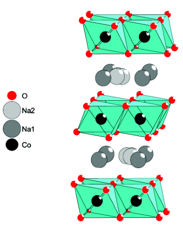
The crystal structure of NaxCoO2 consist on two-dimensional CoO2 layers of edge-sharing tilted octahedra. Each octahedra is composed by a Cobalt ion surrounded by six Oxygen atoms at the vertices CoO6. Within each CoO2 layer, the Co ions occupy the sites of a two-dimensional triangular lattice. The CoO2 layers are separated by insulating layers of Na+ ions. There exist four phases of NaxCoO2, with slightly different structures, called , , and . They differ by the stacking order of CoO2 layers and Na-O environments [61]. In this work we will focus only on the phase because it is the one used in the Hall measurements. Fig. 1.24 shows the structure of the -NaxCoO2, which has an hexagonal structure with a space group symmetry of and lattice constants Å and Å. Band-structure calculations [56] show that the O orbital states lie far below the Co states and the chemical potential falls within the band formed from states in Co. Hence the electrons donated by the Na ions are distributed among the Co ions, a fraction () of which are in the Co4+ state in which , while the rest are Co3+ with . The elementary charge-transport process is the hopping of a hole from Co4+ to Co3+. A large on-site repulsion excludes double occupancy of a site by the holes.

Different ordered states appear as a function of the doping of Na ions. Fig. 1.25 shows the phase diagram for NaxCoO2. A paramagnetic metal is found for and for the system behaves as a Curie-Weiss metal [62]. These two metallic states are separated by a narrow charge-ordered insulating state at . This compound becomes superconducting below K, when intercalated with water forming NaxCoOH2O, for . For values of the doping above , a Spin Density Wave metallic state appears [62, 13]. NaxCoO2 presents also an unusual enhanced thermopower at which has been recently related to the spin entropy carried by the holes in the Curie-Weiss phase [63]. Na0.7CoO2 is the host compound from which Nax is varied to achieve superconductivity in the hydrated compound.
The effective Hubbard interaction have been estimated in band-structure calculations [56] to be of the order of - eV and a Fermi surface with hexagonal character in agreement with photoemission measurements [55, 54]. The dispersion behavior seen in photoemission data is consistent with a negative sign of the single-particle hopping of the order of meV [55]. Therefore, the bandwidth (W) is estimated between to meV making this system a real strongly correlated one with .

Several Hall measurements have been undertaken in Na0.7CoO2 [63, 64]. The anomalous linear increase of the dc Hall coefficient and a recent infrared Hall measurement [64] have motivated recent theoretical works [57, 58, 65, 66] with the aim of investigating the role of correlations in the Hall effect, but many questions remain open. Fig. 1.26 shows the Hall constant measured by Choi et. al. [64] at an infrared frequency and at .
This chapter is the object of publication [67]. In the following we make a theoretical study of the Hall effect in a 2D triangular lattice where electrons interact via an onsite Coulomb repulsion . We calculate in the high frequency limit studied in chapter The Hall effect, and we cover the whole range of interaction values using several approximation schemes.
Model and methods
For this theoretical study, we consider an anisotropic triangular lattice with nearest-neighbor hopping amplitudes and and an on-site Hubbard interaction , with the structure sketched in Fig. 1.27. The system is described by the Hubbard model on the triangular lattice studied in Sec. The 2D triangular lattice:
| (1.177) |
where is the creation (annihilation) fermion operator, is the fermionic number operator and are nearest-neighboring sites. The dispersion relation for this model (see Sec The 2D triangular lattice) is
| (1.178) |
We assume that a current flows along the axis and a dc magnetic field is applied along , hence a Hall voltage develops along the axis (see Fig. 1.27). We use the vector potential , where for the magnetic part we choose, as in the previous chapter, the Landau gauge , and describes the electric field. The coupling between the lattice fermions and the electromagnetic field induces a Peierls phase in the hopping amplitudes which change according to .
We use Eqs. (1.39) and (1.50) for the total current operator, , and the diamagnetic susceptibilities , respectively. Performing the functional derivatives we find for the currents
| (1.179a) | |||||
| (1.179b) | |||||
where we have defined the vector with . The diamagnetic susceptibilities are:
| (1.180b) | |||||
As shown in Sec. The infinite-frequency Hall constant, it is possible to rewrite as a high-frequency series where the infinite-frequency limit reads
| (1.181) |
The remaining contributions are expressed in terms of a memory matrix (see Sec. The Hall constant in the memory function approach). is expected to provide the dominant contribution at any finite frequency. The memory matrix formalism allows in principle to go beyond the infinite frequency approximation and compute corrections at finite frequency [28, 46]. It leads, in particular, to corrections due to interactions that vanish identically if . These corrections do not affect the sign of which should be entirely determined by . In the following we shall consider only the infinite-frequency contribution to , Eq. (1.181), and adopt the notation .
Strictly speaking, our results are valid provided the probing frequency is larger than any other energy scale in the system, . The last two conditions, , are easily fulfilled experimentally in known triangular compounds, while the condition is more problematic. However, as we will discuss in Sec. Discussion and perspectives, in certain limits our results coincide with those obtained in Ref. [57] under the opposite assumption , showing that this condition is not stringent.
In order to evaluate Eq. (1.181), we calculate the commutator from Eqs. (1.179), and we use the diamagnetic susceptibilities of Eq. (1.180) to arrive at
| (1.182) |
with
| (1.183) |
As can be seen from Eq. (1.182) the high frequency Hall coefficient depends only on the distribution function as well as some geometrical factors. The interaction term in Eq. (1.177) therefore only influences through its effect on . Another implication of Eq. (1.182) is that at low temperature the behavior of can be interpreted in terms of an effective carrier concentration, as in the non-interacting case.
Results
In the following we evaluate in the whole domain of interaction values with respect to the bandwidth of the system, by using four different approaches: exact calculation at , a perturbative expansion of the self-energy at , a local approximation to the self-energy, treated with dynamical mean field theory (DMFT) at , and finally the atomic limit of the self-energy at .
Non-interacting case
In the non-interacting case there are various limits in which we can obtain analytical results for ( at ): at zero temperature and band fillings near and , and at high temperature . For intermediate fillings and temperatures, we compute numerically by performing the sum in Eq. (1.182) on a dense discrete -point mesh. Some details on the numerical sum over momentum are given in Appendix Some numerical details.
Zero temperature
Here we restrict for simplicity to the isotropic case and we set the lattice parameter . Close to the band edges we can expand the various integrands of Eq. (1.183) and thus perform the integrals.
Near the bottom of the band the Fermi surface is made of two nearly circular electron pockets around and . In each pocket we have , where is the momentum measured from the pocket center, and therefore . The corresponding electron density is . Writing similar expansions of , , and close to the pocket center and performing the Brillouin zone integrations, we obtain the non-interacting Hall coefficient at low electron density:
| (1.184) |
At sufficiently low density we recover, in the above expression, the classical result .
Near the top of the band the Fermi surface is a nearly circular hole pocket centered at . Close to this point we have , and therefore . The corresponding density is obtained by subtracting the contribution of the hole pocket from the maximum density: . Similarly, for the functions , , and we have to subtract the contribution of the hole pocket from the contribution of the whole Brillouin zone, which turns out to be zero because
| (1.185) |
Thus, for low hole densities we find that the non-interacting Hall coefficient is given by
| (1.186) |
and as we have .
The complete density dependence of calculated numerically at zero temperature from Eq. (1.182) is displayed in Fig. 1.28 and compared to the limiting cases Eqs. (1.184) and (1.186). It is clear from this figure that the infinite-frequency follows the well-known dependence of the dc Hall coefficient on the carrier charge density. This indicates a weak frequency dependence of the non-interacting Hall coefficient at zero temperature, since the dc result is recovered from the infinite frequency limit of . Furthermore this suggests, as we will discuss in more details below, that the frequency dependence should not be too crucial, even in the presence of interactions, for most band fillings. At the sign of the Hall coefficient is entirely given by the sign of the carriers, and it can be seen from Fig. 1.28 how the sign changes at quarter filling when the Fermi energy crosses the van Hove singularity of the DOS, and the Fermi surface shape evolves from electron to hole like.
High temperature
If the distribution function , which reduces to the Fermi distribution at , can be expanded in power of . This expansion must be done at constant density , which requires that remains finite as , in other words at high temperature. Taking this into account we can deduce the relation between and , , and write the Fermi distribution as
| (1.187) |
Due to Eq. (1.185) the -independent terms in Eq. (1.187) do not contribute to , which in this case takes the form:
| (1.188) |
Performing the Brillouin zone integrations we obtain
| (1.189) |
This result is plotted in Fig. 1.29 together with the numerically calculated full temperature and density dependence. The most striking feature of Eq. (1.189) is the linear increase of with . The same linear behavior was obtained in Ref. [68] at , indicating a weak frequency dependence of at high temperature. Our result shows that the -linear dependence of is not due to interactions but to the peculiar topology of the triangular lattice. The sign of at high is determined by the sign of , irrespective of the density (see Fig. 1.29). We attribute this property to the fact that at high enough temperature the full band contributes to the Hall effect; hence the sign of reflects the dominant nature, electron or hole-like, of the band. As is clear from Fig. 1.27, for the band is dominantly hole-like, while for it is electron-like.
The relevance of result (1.189) is that even without interactions, the Hall coefficient has a linear dependence at high temperature due to the geometry of the system, emphasizing the peculiarity of the triangular lattice. By contrast, on the square lattice the same analysis yields a -independent non-interacting at high temperature.
Weakly interacting regime
When interactions are present, the distribution function can be expressed in terms of the one-electron self-energy as:[2]
| (1.190) |
with the odd Matsubara frequencies. In the weak coupling regime , we evaluate the self-energy using conventional perturbation theory in and we keep only the lowest order contributions of order . For a local interaction like the Hubbard term in Eq. (1.177) there is only one diagram which is drawn in Fig. 1.30. The standard diagrammatic rules yield the following expression for the self-energy:
| (1.191) | |||
where is the Fermi distribution function.

The numerical evaluation of Eq. (1.191) is demanding due to the double momentum integration. This is particularly time consuming because our calculations are done at fixed density, and thus require to calculate many times in order to determine the chemical potential. However it turns out that the momentum dependence of in Eq. (1.191) is weak. This is illustrated in Fig. 1.30 where we plot the Brillouin zone average of the self-energy, , as well as its standard deviation. The weak momentum dependence allows us to compute on a coarse (typically ) -point mesh, and then to interpolate using splines (see Appendix Some numerical details) onto a dense mesh for the evaluation of and eventually . The Matsubara sum in Eq. (1.190) also requires special attention: the formal regularization of the divergence through the exponential factor is not suitable for a numerical evaluation of the sum. We therefore rewrite Eq. (1.190) as
| (1.192) |
The sum is now convergent and can be efficiently calculated via the truncation at some large frequency and the analytical evaluation of the remaining terms using an asymptotic expansion of the self-energy.
The resulting from perturbation theory are valid in the regime , with the bandwidth of the system. As already anticipated the effect of a small on the distribution is a subtle broadening, and as a result the dependence of on is very weak at low . Fig. 1.31 provides an illustration of this weak dependence. As a consequence the non-interacting results of Sec. Non-interacting case are expected to give a fairly good account of the Hall effect for an interaction strength smaller than the bandwidth .
An important observation which we can make from our perturbative calculations is that the momentum dependence of the self-energy is very small, i.e. the self-energy is almost local in real space. This suggests to approach the strong-coupling regime by assuming that the self-energy is exactly local. In the following section we study such local approximations to the self-energy, and we compare them to the result of the perturbation theory.
Strongly interacting regime
Assuming that the self-energy is local in first approximation, we investigate here two models for and their implications for the Hall coefficient . The first approach is based on the dynamical mean field theory (DMFT) [6] and requires to solve a difficult self-consistent quantum impurity problem. Due to numerical difficulties this method cannot be pushed to very high interactions and/or very low temperature. Our second approach is based on a simple analytical form for , which is expected to be valid at , and allows us to express analytically in this limit.
DMFT
The DMFT approximation provides the exact solution of the problem under the assumption that the self-energy is local. In this framework the self-energy is expressed as:
| (1.193) |
where is an effective propagator describing the time evolution of the fermions in the absence of interaction, and is the full propagator, which takes into account the local Hubbard interaction. The calculation of from a given amounts to solve the problem of a quantum impurity embedded in a bath. We do it by means of the quantum Monte Carlo Hirsh-Fye algorithm [69] as described in Ref. [6] (see Appendix Calculation of the DMFT self-energy). From the requirement that coincides with the local Green’s function of the lattice, i.e.
| (1.194) |
one can deduce the self-consistency condition
| (1.195) |
where is the Hilbert transform of the DOS corresponding to the triangular lattice and shown in Fig. 1.27. Once the self-consistent is obtained, the corresponding self-energy is injected in Eq. (1.192) to compute .
In Fig. 1.30 we compare the DMFT self-energy with the Brillouin zone average of the perturbative expression Eq. (1.191), both calculated at . It can be seen that the frequency dependence and the order of magnitude of the two quantities are very similar, suggesting that the self-energy is dominated by the term and therefore the domain of validity of the perturbation theory is not limited to very small . On the other hand it shows that the DMFT, although it is not a perturbative approach, provides a smooth transition from the weak to the strong-coupling regimes. This is further illustrated in Fig. 1.31 where we see that the values of calculated by perturbation theory and DMFT coincide up to . At not too low temperature the DMFT calculation is reliable up to interaction strengths comparable to the bandwidth . We have performed DMFT calculations at , but since these results could be affected by systematic statistical errors in the Monte-Carlo summation, they are not shown in Fig. 1.31 (Appendix Calculation of the DMFT self-energy). At it is expected that the DMFT result approaches the atomic limit in which accurate calculations can be performed, as discussed in the next paragraph.
Atomic limit
In the limit of very strong interactions we assume that the self-energy approaches its atomic limit given by the expression: (see Appendix Self-energy and distribution function in the atomic limit):
| (1.196) |
with the chemical potential in the atomic limit, not to be confused with the lattice chemical potential . Using this expression in Eq. (1.190) it is possible to evaluate analytically the sum over Matsubara frequencies and thus to obtain a closed expression for (Appendix Self-energy and distribution function in the atomic limit). In Fig. 1.31 we show the Hall coefficient calculated with the atomic limit of the self-energy in the whole range of interaction values. obviously converges to the non-interacting limit at low since the atomic self-energy vanishes at , and provides a good interpolation between the weak and the strong-coupling regimes. At intermediate values the atomic limit is not reliable, although it gives the correct order of magnitude for . Fig. 1.31 also shows that saturates at sufficiently large .
In Fig. 1.32 we display the temperature and density dependence of at , which is a typical value for the cobaltate compounds as discussed in the next section. We have selected four densities corresponding to the bottom and top of the lower and upper Hubbard bands (see also Fig. 1.34 below). Like for we find a -linear increase of at . Due to the Mott gap, however, the density dependence of the slope is not the same as for . The slope can be obtained explicitly by sending to and performing the high-temperature expansion as in Sec. High temperature The result is
| (1.197) |
very similar to Eq. (1.189) except that the slope replaces , where measures the departure from half-filling. The result of Eq. (1.197) is displayed in Fig. 1.32, and correctly describes our high-temperature results at . The differences observed at in Fig. 1.32 reflect the fact that close to half-filling the slope of the high temperature depends strongly on the interaction and is not saturated even at (see also Fig. 7). Away from half-filling the dependence of the slope is weaker, and Eq. (1.197) is valid for lower interaction values.
Discussion and perspectives
The various approximations presented above allow us to calculate the Hall coefficient on the triangular lattice for all interactions strengths and all temperatures . The main limitation of our approach, in view of a comparison with experimental systems, is that our results are in principle valid in the limit , because they are based on a high-frequency expansion. The first criterion, , is not too difficult to satisfy for realistic compounds if the measurement of the Hall effect is performed at optical frequencies. The second criterion, , seems more problematic since interaction strengths can be as large as several electron volts, at the upper edge of the mid-ultraviolet frequency domain. However, we have seen (Fig. 1.28) that at and the Hall coefficient calculated at coincides with the dc value, and at and , we obtained the results of Ref. [68]. All this suggests that the frequency dependence of is weak in the non-interacting case.
At the other extreme of the parameter space, and , we can compare the result of the atomic limit approximation with the result of the - model [57]. In the latter model is considered infinite from the outset, so that the high-frequency and high temperature expansion of Ref. [57] is in fact valid at frequencies . We plot in Fig. 1.33 the density dependence of obtained in both models at and . The small quantitative difference between the atomic limit at and the - model shows that these two ways of treating the limit are not equivalent: they differ, in particular, in the renormalization of the kinetic energy by the interaction. However the two models give away from half filling very similar behaviors. This reinforces the idea that the frequency dependence of is weak. Exact diagonalization on small clusters also indicate such a weak frequency dependence [58]. This strongly suggests that our results could also be valid at , and therefore be relevant to interpret experiments performed in this regime.
The atomic-limit approach has the advantage to give access to the full temperature dependence (Fig. 1.32) as well as the -dependence as shown in Fig. 1.33, while the calculation of Ref. [57] is valid at and .
The evolution of with temperature is of particular interest since it is most easily probed experimentally. A linear increase of with temperature, without saturation at high , was reported in Ref. [57] for the - model. Our results show that the Coulomb interaction is not responsible for this effect which is also present at (Fig. 1.29) and is therefore a consequence of the peculiar geometry of the triangular lattice. However the interaction controls the density dependence of the slope which changes smoothly from at to at . This is further corroborated in Fig. 1.33.
The sign of turns out to be independent of and at high temperature, unlike in the square lattice where changes sign at . The situation is different at . In the non-interacting case changes sign at quarter filling and can be simply interpreted in terms of the carrier density (Fig. 1.28). We have also investigated the density dependence of at large as shown in Fig. 1.34. The interpretation in terms of the carrier density remains qualitatively valid, provided one takes into account the splitting of the DOS into the lower and upper Hubbard bands. These two bands are displayed in Fig. 1.34b, where it can also be seen that the DOS keeps qualitatively the same shape as for , but the width of each band varies strongly with the density . Due to this band renormalization the sign change of at does not occur at quarter filling, but a little below. Comparing Fig. 1.34a with Fig. 1.33 one easily understands why the temperature dependence of is more pronounced slightly above and , where changes from negative at to positive at high , than slightly below and where its stays positive (see also Fig. 1.32).
Let us now discuss the application of our theoretical results to the Hall measurements performed at finite frequency by Choi et al. [64] on the cobaltate Na0.7CoO2 (see Fig. 1.26). As mentioned before, ARPES measurements [55] indicate that the triangular lattice is isotropic with an estimated hopping amplitude of meV and an effective Hubbard energy eV. From the radius of the Fermi-surface hole pocket observed in ARPES, Å-1, we deduce an electron density . Choi et al. measured the temperature dependence of both the dc and ac Hall coefficients up to room temperature (see Fig. 1.26). The ac measurement was performed at cm. The experimental conditions thus satisfy . In Fig. 1.35 we plotted together the experimental and theoretical curves. As can be seen in the figure, there is a factor of between the measured at finite and zero frequency. The order of magnitude of our theoretical curve, obtained with the parameters measured with ARPES, is in agreement with the dc Hall data and not with the ac Hall data, as expected. We do not have, at the moment, any clear explanation for this discrepancy. One would have to extend the theoretical approach in order to cover the domain of intermediate frequencies and more infrared measurements are needed in order to assure that the experimental data is correct. In any case, we compare our results with the dc Hall data at high temperatures and the results are discussed below.
The behavior of the dc above K is consistent with the linear increase predicted by the various theoretical models. By adjusting these models on the dc experimental data at high temperature (dotted line in Fig. 1.35) we obtain independent determinations of the hopping amplitude , namely meV using the atomic limit model Eq. (1.197) and meV using the - model. This values are in good agreement with the ARPES results. We note, however, that there are discrepancies between different sets of experimental data [64, 63].
The organic conductors of the BEDT family present several compounds with an anisotropic triangular structure. Unfortunately we are not aware of any measurements of the ac Hall effect which we could compare to our calculations, although measurements have been done at zero frequency in these materials.[70, 71]
Conclusions
The theoretical high-frequency Hall coefficient in the two-dimensional triangular lattice exhibits two different characteristic behaviors at low and high temperatures: near , resembles the classical dc Hall coefficient where and are the carrier charge and density, respectively; at temperatures higher than the bandwidth, shows a remarkable -linear behavior with a density- and interaction-dependent slope. These conclusions apply provided the probing frequency is larger that the other energy scales of the problem, and that the electron self-energy remains essentially local for strong interactions.
Although we argued that the frequency dependence of is probably weak, it is clear that for understanding the anomalously large measured experimentally in Na0.7CoO2 in the mid-infrared range, one would have to extend the approach in order to cover the domain of intermediate frequencies. Concerning the self-energy, we do not exclude that this quantity could present a non-negligible momentum dependence for strong interactions. This could affect the Hall coefficient, especially at low temperature. Such a momentum dependence is indeed expected for ordered ground states at and close to half-filling due to antiferromagnetism. However, the influence of a momentum-dependent self-energy would be reduced on the Hall effect, because the expression Eq. (1.182) for the Hall coefficient averages the distribution function over the Brillouin zone. In addition we do not expect a strong momentum dependence far from half-filling, as in the case of the cobaltate considered here.
Another possibility is that the simple one-band model considered in this study would not suffice to capture the detailed properties of the materials [72]. Experiments conducted as a function of , as well as measurements of other materials with a triangular structure, would be very helpful to elucidate the peculiarities of the Hall effect in triangular compounds.
Conclusions
This work was devoted to the investigation of the Hall effect in
two different theoretical models of strongly correlated systems: a
system made of weakly coupled Luttinger liquids and the
two-dimensional triangular lattice. In order to have the necessary
theoretical tools to tackle these problems, we started with a
review on the main properties of systems with strong interactions,
focusing on two-dimensional and low-dimensional systems (1D and
quasi 1D). Because the Hall effect is first of all a transport
phenomenon, we reviewed the formalisms existing in the literature
to treat transport properties in strongly interacting systems, and
we dedicated a whole chapter to the specific treatment of the Hall
effect. The conclusions corresponding to each of the models
studied are presented in what follows.
The study of the Hall effect in a quasi 1D system was in part
motivated by various Hall measurements made on quasi 1D organic
conductors. This work consisted on the application of the memory
matrix formalism to obtain the Hall constant () in weakly
coupled -filled chains, in the presence of umklapp
scattering. The geometry of the model was chosen in order to have
the current flowing along the 1D chains. We computed the
temperature and frequency dependence of taking into account
particle-particle interactions and particle-lattice interactions
(umklapp processes). We obtained a Hall coefficient given by
the free-fermion value (band value ) plus a correction term
with a power-law dependence on temperature (or frequency), due to
the presence of umklapp scattering. These power-law dependencies
are signatures of Luttinger liquid behavior, where the exponents
depend on the interaction parameters. The Hall coefficient was
also computed for the system without forward scattering
(particle-particle interaction), resulting in a logarithmic
dependence on (or ), in agreement with the zero
interaction limit of the power-law. Because the organic conductors
are -filled and - filled systems at the same time, our
theoretical results are not directly applicable to explain the
available Hall data, but they allowed us to make valuable
conclusions. Firstly, the proper way to analyze the Hall data,
made in such quasi-1D systems (in the same geometry of our model),
is to fit the deviations from the band value starting from
the high temperature limit. And secondly, signatures of LL
behavior (power-law dependence) are expected to appear, at high
temperatures, in Hall measurements made in the geometry considered
here. A second geometry, where the magnetic field is applied along
the 1D chains, can be considered for this system and the question
of the appearance of LL signatures in this case remains open.
The second model studied in this work was the two-dimensional
triangular lattice with an onsite interaction . This
theoretical study was partially motivated by Hall experiments made
at finite and zero frequency on the sodium cobalt oxide. We
computed the infinite-frequency Hall constant, where the probing
frequency must be larger that the other energy scales of the
problem, for all interactions strengths and all temperatures
. We obtained an with two different
characteristic behaviors at low and high temperatures: near ,
resembles the classical dc Hall coefficient where
and are the carrier charge and density, respectively; at
temperatures higher than the bandwidth, presented a
-linear behavior with a density- and interaction-dependent
slope. These results were applied to the Hall data measured on
cobaltates at finite (infrared) and zero frequency. The finite
frequency data showed an order of magnitude of difference with our
theoretical results. To understand this discrepancy, one would
have to extend the approach in order to cover the domain of
intermediate frequencies. The behavior of the dc at high
temperature was consistent with the linear increase predicted
theoretically. By adjusting the model on the dc experimental data
at high temperature we obtain independent determinations of the
hopping amplitude in accordance with the experimental values. An
extension to the work done here can be the calculation of the
memory matrix term for the Hall constant to leading order in .
This would give the behavior of the Hall constant at lower
frequencies.
After summarizing the conclusions corresponding to each one of the models studied, we must point out that the study of the Hall effect in strongly correlated system is a very complicated problem from the theoretical point of view. Interactions can have a large effect on the transport properties. In particular, for the Hall resistivity these effects seem to increase when the dimensionality of the system decreases. However, with this work we have learned that there are feasible ways to treat this problem and that each geometry must be treated in a different way. In any case, much more needs to be done in order to understand form a theoretical point of view the large number of experiments and the real meaning of the Hall resistivity in strongly correlated systems.
Appendix for the study of the Hall effect in quasi 1D systems
Correlator at zero order in and
The operators and are given in boson representation in Eqs. (1.159) and (1.161). Here we replace by for right(left) moving fermions in the expression for . To obtain the correlator at zero order in the band curvature term and magnetic field, we take Eq. (1.158) with and we put in expressions (1.159) and (1.161),
| (198) |
We denote by the time-ordered correlation function and the superindice means zero order in . All the terms are multiplied by the factor: . We will use the letter to denote it in the following calculations. In bosonization language, the average (198) gives
| (199) | |||
with Due to result (1.163), the surviving terms are those satisfying , where and are defined in Eq. (1.163). Separating spin and charge parts, we have (the common prefactor is omitted in other to lighten notation)
Now, making explicitly all the products in the above expression we obtain four different terms,
Summing over the spins and , and using the result shown in Eq. (1.163), we finally obtain that at zero order in the band curvature () and magnetic field (), the correlator vanishes,
This can also be verified applying spatial inversion and particle-hole symmetry in correlator
Full expression for the correlator at first order in and
Here we will repeat the same type of calculations done in Appendix Correlator at zero order in and , but in this case we consider the band curvature term in the correlator and we take to first order in the terms depending on the magnetic field ( and ). Thus the correlator is given in Eq. (1.158). Again we take the bosonized form for each operator (see Sec. in the presence of umklapp and forward scattering) and we put all the prefactors together in a constant named . The resulting expression is
| (200) |
There are again four surviving terms, all multiplied by
Summing over the spins and , and using result (1.163) we write the above expressions in terms of functions and
| (201) |
The functions and are given in Eq. (1.164). The factor is the behavior of at large distances [16]. Because the model studied in Sec. in the presence of umklapp and forward scattering is spin rotational invariant, we have . The function gives the angular part in the above expression and thus, does not play any role in the scaling analysis, where only power-law dependencies are involved. Keeping only the terms with functions and making the following change of variables: , , and ; we obtain result (1.166). We take only the magnitude for in the prefactor because, as we said before, angular parts can be neglected in the scaling analysis.
Full expression for with
For the analytical obtention of correlator with , we will need in several instances the average value to first order in . We note that in the absence of magnetic field this quantity equals the free Green’s function of the 2D lattice:
With a finite magnetic field we can use another method: in general, in the presence of a time-independent perturbation, the Green’s function obeys Dyson’s equation: . In our case is the Green’s function in the absence of interaction and for , i.e. with the chain index. On the other hand, the self-energy is simply . The magnetic field enters in the shift of momentum . At first order in , we have:
| (202) | |||||
Thus, we obtain an expression for the Green’s function to first order in and in presence of a magnetic field ,
| (203) | |||||
This last expression reduces to our previous result if . The result (203) will be used in the following computation of the correlator . Starting from Eq. (1.171), we write the complete expression for correlator
| (204) | |||
In the first parenthesis the operators are evaluated at position and time , while in the second parenthesis they are at position and time . We consider the first term:
| (205) |
We can decouple this term in only two different ways. The first is
| (206) |
and it clearly implies that and . The chain indices and must be such that the fermions are on the same or nearest-neighbor chains, since we work at first order in . The only solution is , since the other possibility, , gives a term of order . Hence the term reads
| (207) |
with the free propagator. Using Eq. (203), we find that the first decoupling yields the following contribution to [we temporarily omit the prefactor in Eq. (204)]:
| (208) | |||||
This corresponds to the diagram shown in Fig. 1.23. The 2nd decoupling of Eq. (205) is
| (209) |
and implies , , and :
| (210) |
This is the same expression as for the first decoupling provided we change into . It will therefore give the same contribution .
We now move to the second term:
| (211) |
Again there are only two decoupling:
The calculation is very similar to the previous one: just exchange and and add a minus sign. Hence these two terms contribute
| (212) | |||||
where we have used the fact that . The third term is
| (213) |
and can be decoupled as follows
Both terms are equivalent except for the sign of . From Eq. (202) we read that
| (214) |
and we then find that these two terms contribute . We continue the game with the fourth term:
| (215) |
which has the decoupling
and contributes . There are four additional terms to consider, for which we look only at the first of the two equivalent decoupling:
| (216) | |||||
| (217) | |||||
| (218) | |||||
| (219) | |||||
At this point we have calculate all the terms and we have found that
| (220) |
It is clear enough that vanishes at . The first-order term is
| (221) |
with . For this implies
| (222) |
The last step is to evaluate :
The Matsubara sums are elementary (once third-order poles are under control, and yield
where is the Fermi function . At this stage we shift and by , and by . Then the energy of the right movers , which depend only on one momentum, becomes . At the same time becomes , and finally becomes . This last equality holds because we are at half-filling so that . We also move to adimensional variables :
| (223) |
where and the ’s and are the ’s and with momenta replaced by and replaced by . For example, must be replaced by . We see that the temperature disappears completely from the momentum integrals. We then take away the tildes and rewrite:
| (224) | |||||
We treat this expression to first order in . For this we introduce a new quantity: , in such a way that . Taking into account the various factors we arrive at
| (225) |
Taking the imaginary part in Eqs (225) and (224) leads to delta functions which allows one to do the integration directly using the identity:
| (226) |
The remaining and integrals can be done exactly yielding
| (227) |
We see that the integrand becomes at high frequency, and therefore the integral diverges as where is the cutoff. We can extract the divergent term by rewriting the integral as
Our final result is thus
| (228) |
Appendix for the study of the Hall effect on the triangular lattice
Some numerical details
To obtain the full temperature and density dependence of
using Eq (1.182) we computed the sum over momentum
numerically. For this we took a reduced zone of the reciprocal
space of the 2D triangular lattice, defined by vectors
and
(see
Sec. The 2D triangular lattice). We then performed an grid discretization of this zone (discrete mesh), with the total
number of sites. Due to the -periodicity of coefficients
, and , and that of
dispersion relation , which are the
-dependent quantities in Eq (1.182), it can be
proved that for the description of the whole reciprocal space, is
enough to make the sum over a triangle defined by points
P; P and
P. Each -point in the triangle
must be weighted according to the number of times it appears when
the full reduced zone is recovered, by making reflections of the
triangle. In the following, some short routines are presented
(written in fortran 95). They allow to obtain the diamagnetic
terms and therefore (in unities of with
c=1) at . In this routines, "Nt" denotes the number of sites (the total number given by Nt2)
and "dist" is the Fermi distribution function (where the
temperature and density enter),
function p(Nt) (gives the proper weigh to each point in the
triangle)
Implicit None
integer, intent(in) :: Nt
integer, dimension((Nt/2+2)*Nt/2) :: p
integer :: i,m
p=4; p(1:Nt-1)=2
do i=1,Nt/2; m=i*(Nt-(i-2)); p(m)=2; p(m-1)=2
enddo
p(Nt)=1 ; p((2+Nt/2)*Nt/2)=1
end function p
This funtion is used in the two following routines.
function X(dist) ( returns the diamagnetic terms and )
Implicit None
real,dimension(:),intent(in) :: dist
real, dimension(2):: X
integer, dimension((Nt/2+2)*Nt/2) :: wei
integer :: k,ki,kj
real:: kx,ky
wei=p(Nt) ; X = zero
do k=1,size(dist)
kj=floor((Nt+two)/2-sqrt((Nt+two)**2/4-k)+1.d-10)
ki=k-kj*(Nt-kj)
kx=mod(ki,Nt)*two*pi/(a*Nt)
ky=(-mod(ki,Nt)+2*kj)*two*pi/(a*Nt*sqrt(3.d0))
X(1)=X(1)+wei(k)*(two*cos(kx*a)+
(tper/tpar)*cos(kx*a/two)*cos(ky*sqrt(3.d0)*a/two))*dist(k)
X(2)=X(2)+wei(k)*cos(kx*a/two)*cos(ky*sqrt(3.d0)*a/two)*dist(k)
enddo
X(1)= X(1)/Nt**2 ; X(2)= X(2)/Nt**2
end function X
Once we have the diamagnetic terms, we are ready to compute the Hall coefficient by means of the following routine.
function RH(dist) (returns the Hall constant
)
Implicit None
real(dp),dimension(:),intent(in) :: dist
real(dp), dimension(2):: diamag
real(dp) :: RH,term1,term2,kx,ky
integer, dimension((Nt/2+2)*Nt/2) :: wei
integer:: k,ki,kj
diamag=X(dist); RH= zero; term1=zero; term2=zero; wei=p(Nt)
do k=1,size(dist)
kj=floor((Nt+two)/2-sqrt((Nt+two)**2/4-k)+1.d-10)
ki=k-kj*(Nt-kj)
kx=mod(ki,Nt)*two*pi/(a*Nt)
ky=(-mod(ki,Nt)+2*kj)*two*pi/(a*Nt*sqrt(3.d0))
term1=term1+
wei(k)*cos(kx*a)*cos(kx*a/two)*cos(ky*sqrt(3.d0)*a/two)*dist(k)
term2=term2+
wei(k)*(cos(kx*a)+cos(ky*sqrt(3.d0)*a))*dist(k)/4.d0
enddo
RH = -((a**2)*sqrt(3.d0)/2.d0)*(term1+
(tper/tpar)*term2)/(diamag(1)*diamag(2)*Nt**2)
end function RH
In the case, the above routines must be adapted to obtain
the self-energy and consequently ,
with the different methods explained in Sec. Results.
Due to the weak momentum of , we can
compute it in a mesh and then, using the function
shown below, interpolate it into an mesh as large as
possible (in our work ):
function spline (v1,v2,A) (returns a linear interpolation of the array A to the vector v) (v1 must
be in the range [0,size(A,1)] and v2 in the range [0,size(A,2)].)
Implicit None
real(dp), intent(in) :: v1, v2
complex(dp), dimension(0:,0:), intent(in) :: A
complex(dp) :: spline
integer :: N, M, i, j; real(dp) x, y
complex(dp) :: A1, A2, A3,
A4
N=size(A,1); M=size(A,2)
if(v1<zero.or.v1>real(N,dp)) then
stop ’Stopped => Out-of-range vector v1 in lib:spline’
else if(v2<zero.or.v2>real(M,dp)) then
stop ’Stopped => Out-of-range vector v2 in lib:spline’
endif
i=int(v1); j=int(v2); x=v1-i; y=v2-j; i=mod(i,N);
j=mod(j,M)
A1=A(i,j); A2=A(mod(i+1,N),j)
A3=A(mod(i+1,N),mod(j+1,M)); A4=A(i,mod(j+1,M))
spline=A1+(A2-A1)*x+(A4-A1)*y+(A1-A2+A3-A4)*x*y
end function spline
Then, for each element of the original complex matrix we find by interpolation the element with the size of the final matrix we want to obtain. In the above routine, v1, v2 and A correspond to , and respectively.
Calculation of the DMFT self-energy
We evaluate the local self-energy in the DMFT framework using the Hirsh-Fye algorithm [69] as described in Ref. [6]. In this method the imaginary-time axis is cut into slices, and the Trotter formula is used in each time slice in order to single out the Hubbard interaction. In a second step the interaction is decoupled via the introduction of an Ising variable in every time slice. The Green’s function is finally calculated by averaging over the ensemble of configurations of the Ising variables using a Monte-Carlo sampling and local updates. In our calculations at and we take and we keep out of the configurations visited. The numerical accuracy of the calculated is estimated to be at the highest values, and closer to at . We believe that the accuracy at is not sufficient to get a reliable self-energy; hence we did not evaluate at in Fig. 1.31.
In order to calculate the self-energy and solve the DMFT self-consistency condition, Eq. (1.195), we need to Fourier transform from imaginary time to imaginary Matsubara frequencies . In traditional implementations of the algorithm this step is performed through a cubic spline interpolation of . Because cubic splines are non-analytic, however, the resulting Fourier series are unreliable at frequencies above . Instead of an interpolation, we have performed a fit of . Our fitting function is a discrete form of the spectral representation, , which we express as
| (229) |
with and . The number of poles and their weight are determined by adding more and more terms in Eq. (229), until the fitted function matches all QMC data points within a numerical tolerance, which we take as the estimated accuracy of . The Fourier transform is then simply
| (230) |
The calculated self-consistent propagators and are displayed in Fig. 36, together with the fits to Eq. (229).
Solving Eq. (1.195) at fixed electron density requires to determine the chemical potential self-consistently. In our calculations we perform the search for both the self-consistent and in one shot using a global minimization procedure. As a result the self-consistent solution can be reached in typically less that 20 iterations.
Self-energy and distribution function in the atomic limit
In the case one can treat the Hamiltonian Eq. (1.177) using a perturbative expansion in . The atomic limit is the zeroth-order term of this development, and it corresponds to a collection of disconnected sites with four possible states on each site. This limit is not very useful since there is no hopping and thus no possible transition below the Hubbard energy . In order to retain the low-energy dynamics of the problem we adopt an hybrid approach, where the free dispersion is used in the lattice Green’s function together with the self-energy evaluated in the atomic limit. The atomic self-energy is obtained by diagonalizing the Hamiltonian Eq. (1.177) with , which leads to the atomic Green’s function
| (231) |
while the non-interacting results by putting . From Dyson’s equation, , we deduce the atomic self-energy displayed in Eq. (1.196). Here is the chemical potential in the true atomic limit—i.e. the limit where the lattice Green’s function takes the form (231), and therefore the electron density is given by with the Fermi function. We can invert this relation and express explicitly in terms of the electron density as
Using the atomic self-energy Eq. (1.196) as an approximation to the exact self-energy in Eq. (1.190), we evaluate analytically the lattice distribution function . Let’s first remark that
with
As a result the Matsubara sum in Eq. (1.190) is easily performed to yield
| (232) |
Within this approximation it is also straightforward to perform the infinite limit. Taking into account that both and are either of order (if ) or of order (if ) we find that approaches as increases toward . Likewise, if we have and while if we have and . Hence we find
where we have introduced and with . For the purpose of evaluating the high-temperature behavior of the Hall coefficient at , we finally expand the distribution function in powers of following the procedure described in Sec. High temperature:
Comparing with Eq. (1.187), which is valid at , we see that the only difference between the high-temperature behaviors of at and is the -dependent slope, and we easily deduce that
By introducing which measures the doping with respect to half-filling, these two cases can be recast in one single expression shown in Eq. (1.197).
Acknowledgements
This PhD thesis would not have been possible without the help and support of the people around me, to only some of whom it is possible to give particular mention here.
Above all, I would like to thank my principal supervisor, Prof. Thierry Giamarchi, who gave me the opportunity to come to Switzerland for the accomplishment of this research. His hard work, support, enthusiasm and scholarship have set an example I hope to match someday. The patience, support and dedication of my second advisor, Dr. Christophe Berthod, has been invaluable for the achievement of this thesis, for which I am extremely grateful.
I am also grateful to Prof. Andrew Millis who visited us for six month and collaborated intensively in the second part of this work. I would like to thank Prof. B. S. Shastry, Prof. H. D. Drew and Prof. S. Brown for valuable discussions.
I would like to acknowledge the financial support given by the Swiss National Science Foundation through Division II and MaNEP, and the finantial and academic support of the Université de Genève, in particular the Condensed Matter Physics Department and its staff.
Specials thank to my colleagues in Giamarchi’s group: Anibal, Alejandro, Corinna, Sebastian, Alejandro, Pierre, Vivien, Elisabeth and Mikhail; and those at the Ecole de Physique: Dook, Heidi, Anna-Sabina, Alexander, Giorgio, Pablo, Yanina, Silvia, Noé; for their kind support and friendship along these four years in Geneva.
I would like to thank also the VTT group of the Ecole de Physique: Charly, Robert, Géraldine, Loren, Enrico, Tania, Alexander; with whom I discovered the countryside of Geneva and Switzerland.
Special thanks to Aisha, Yamila, Aurélie and others that I have already mentioned, for making life outside work much more fun. And so many thanks to the group of Torino, where I spent so unforgettable weekends during my Ph.D. I would like to thank also my friends from Caracas, you will always be in my heart.
Finally, I have no words to express the gratitude that I feel to my parents, Chichi and Rina, who have taught me everything I know about life; to my brother, Edel, who gives me so much energy to continue every day and to my lovely Jose Enrique, who makes my life so joyful. This thesis is dedicated to you, my family.
References
- [1] Landau, L. D. Sov. Phys. JETP 8, 70 (1958).
- [2] Mahan, G. D. Many Particle Physics. Plenum, New York, (1981).
- [3] Nozieres, P. Theory of Interacting Fermi Systems. Benjamin, New York, (1961).
- [4] Lieb, E. H. and Wu, F. Y. Phys. Rev. Lett. 20, 1445 (1968).
- [5] Marder, M. P. Condensed Matter Physics. Wiley-Interscience, New York, (2000).
- [6] Georges, A., Kotliar, G., Krauth, W., and Rozenberg, M. J. Rev. Mod. Phys. 68, 13 (1996).
- [7] Mott, N. F. Proc. Phys. Soc. Sect. A 62, 416 (1949).
- [8] Mott, N. F. Metal–Insulator Transitions. Taylor and Francis, London, (1990).
- [9] Hirsch, J. E. Phys. Rev. Lett. 54, 1317 (1985).
- [10] Matsumoto, H., Saikawa, T., and Mancini, F. Phys. Rev. B 54, 14445 (1996).
- [11] Kotliar, G. and Liu, J. Phys. Rev. B 38, 5142 (1988).
- [12] Ashcroft, N. and Mermin, N. Solid State Physics. Saunders College, Philadelphia, (1976).
- [13] Ong, N. P. and Cava, R. J. Science 305, 52 (2004).
- [14] Haldane, F. D. M. J. Phys. C 14, 2585 (1981).
- [15] von Delft, J. and Schoeller, H. Ann. Phys. 7, 225 (1998).
- [16] Giamarchi, T. Quantum Physics in One Dimension. Oxford University Press, Oxford, (2004).
- [17] Giamarchi, T. Chem. Rev. 104, 5037 (2004).
- [18] Luttinger, J. M. J. Math. Phys. 4, 1154 (1963).
- [19] Anderson, P. W. J. Phys. C 3, 2346 (1970).
- [20] Schulz, H. J. Phys. Rev. Lett. 77, 2790 (1996).
- [21] Götze, W. and Wölfle, P. Phys. Rev. B 6, 1226 (1972).
- [22] Fick, E. and Sauermann, G. The Quantum Statistics of Dynamic Processes. Springer, Berlin, (1990).
- [23] Giamarchi, T. Phys. Rev. B 44, 2905 (1991).
- [24] Negele, J. W. and Orland, H. Quantum Many–Particle Systems. Frontiers in Physics. Addison–Wesley, Reading, MA, (1988).
- [25] Lopatin, A., Georges, A., and Giamarchi, T. Phys. Rev. B 63, 075109 (2001).
- [26] Georges, A., Giamarchi, T., and Sandler, N. Phys. Rev. B 61, 16393 (2000).
- [27] Shastry, B. S., Shraiman, B. I., and Singh, R. R. Phys. Rev. Lett. 70, 2004 (1993).
- [28] Lange, E. Phys. Rev. B 55, 3907 (1997).
- [29] Jérome, D. Chem. Rev. 104, 5565 (2004).
- [30] Dresselhaus, M. S., Dresselhaus, G., and Eklund, P. C. Science of Fullerenes and Carbon Nanotubes. Academic Press, San Diego, CA, (1995).
- [31] Stöferle, T., Moritz, H., Schori, C., Köhl, M., and Esslinger, T. Phys. Rev. Lett. 92, 130403 (2004).
- [32] B�ssler, H. Nature 2, 15 (2006).
- [33] Julien, F. H. and Alexandrou, A. Science 282, 1429 (1998).
- [34] McEuen, P. L. Science 278, 1729 (1997).
- [35] Mori, T. Chem. Rev. 104, 4947 (2004).
- [36] Dressel, M. Science 90, 337 (2003).
- [37] Schwartz, A., Dressel, M., Grüner, G., Vescoli, V., Degiorgi, L., and Giamarchi, T. Phys. Rev. B 58, 1261 (1998).
- [38] Giamarchi, T. Physica B 230-232, 975 (1997).
- [39] Vescoli, V., Zwick, F., Henderson, W., DeGiorgi, L., Grioni, M., Gruner, G., and Montgomery, L. K. Eur. Phys. J. B 13, 503 (2000).
- [40] Moser, J., Gabay, M., Aubin-Senzier, P., Jérome, D., Bechgaard, K., and Fabre, J. Eur. Phys. J. B 1, 39 (1998).
- [41] Henderson, W., Vescoli, V., Tran, P., Degiorgi, L., and Grüner, G. Eur. Phys. J. B 11, 365 (1999).
- [42] Moser, J., Cooper, J. R., Jérome, D., Alavi, B., Brown, S., and Bechgaard, K. Phys. Rev. Lett. 84, 2674 (2000).
- [43] Mihaly, G., Kezsmarsky, I., Zamborsky, F., and Forro, L. Phys. Rev. Lett. 84, 2670 (2000).
- [44] Korin-Hamzić, B., Tafra, E., Basletić, M., Hamzić, A., Untereiner, G., and Dressel, M. Phys. Rev. B 67, 014513 (2003).
- [45] Korin-Hamzić, B., Tafra, E., Basletić, M., Hamzić, A., and Dressel, M. Phys. Rev. B 73, 115102 (2006).
- [46] León, G., Berthod, C., and Giamarchi, T. Phys. Rev. B 75, 195123 (2007).
- [47] León, G. and Giamarchi, T. J. Low Temp. Phys 142, 315 (2006).
- [48] Haldane, F. D. M. J. Phys. C 14, 2585 (1981).
- [49] Yakovenko, V. M. Synth. Metal 103, 2202 (1999).
- [50] Heuzé, K., Fourmigué, M., Batail, P., Coulon, C., Clérac, R., Canadell, E., Auban-Senzier, P., Ravy, S., and Jérome, D. Adv. Mater. 15, 1251 (2003).
- [51] Anderson, P. W. Science 235, 1196 (1987).
- [52] Takada, K., Sakurai, H., Takayama-Muromachi, E., Izumi, F., Dilanian, R. A., and Sasaki, T. Nature 422, 53 (2003).
- [53] Qian, D., Wray, L., Hsieh, D., L.Viciu, Cava, R. J., Luo, J. L., Wu, D., Wang, N. L., and Hasan, M. Z. Phys. Rev. Lett. 97, 186405 (2006).
- [54] Laverock, J., Dugdale, S. B., Duffy, J., Wooldridge, J., Balakrishnan, G., Lees, M. R., Zheng, G., Chen, D., Lin, C. T., Andrejczuck, A., Itou, M., and Sakurai, Y. Phys. Rev. B 76, 052509 (2007).
- [55] Hasan, M., Chuang, Y.-D., Qian, D., Li, Y., Kong, Y., Kuprin, A., Fedorov, A., Kimmerling, R., Rotenberg, E., Rossnagel, K., Hussain, Z., Koh, H., Rogado, N., Foo, M., and Cava, R. Phys. Rev. Lett. 92, 246402 (2004).
- [56] Singh, D. Phys. Rev. B 61, 13397 (2000).
- [57] Kumar, B. and Shastry, B. S. Phys. Rev. B 68, 104508 (2003).
- [58] Haerter, J. O., Peterson, M. R., and Shastry, B. S. Phys. Rev. B 74, 245118 (2006).
- [59] Seo, H., Hotta, C., and Fukuyama, H. Chem. Rev. 104, 5005 (2004).
- [60] Vaulx, C. Etude par R�sonance Magn�tique Nucl�aire de Cobaltates NaxCoO2. PhD thesis, Universit� Joseph Fourier - Grenoble I, (2007).
- [61] Son, J. Y., Kim, B. G., and Chon, J. H. Appl. Phys. Lett. 86, 221918 (2005).
- [62] Foo, M. L., Wang, Y., Watauchi, S., Zandbergen, H. W., He, T., Cava, R. J., and Ong, N. P. Phys. Rev. Lett. 92, 247001 (2004).
- [63] Wang, Y., Rogado, N. S., Cava, R. J., and Ong, N. P. Nature 423, 425 (2003).
- [64] Choi, E., Jung, S., Noh, J., Zimmers, A., Schmadel, D., Drew, H., Bang, Y., Son, J., and Cho, J. Phys. Rev. B 76, 033105 (2007).
- [65] Haerter, J. O., Peterson, M. R., and Shastry, B. S. Phys. Rev. Lett. 97, 226402 (2006).
- [66] Koshibae, W., Oguri, A., and Maekawa, S. Phys. Rev. B 75, 205115 (2007).
- [67] León, G., Berthod, C., Giamarchi, T., and Millis, A. Phys. Rev. B 78, 085105 (2008).
- [68] Motrunich, O. I. and Lee, P. Phys. Rev. B 69, 214516 (2004).
- [69] Hirsch, J. E. and Fye, R. M. Phys. Rev. Lett. 56, 2521 (1986).
- [70] Sushko, Y. V., Shirakawa, N., Murata, K., Kubo, Y., Kushch, N. D., and Yagubskii, E. B. Synth. Metal 85, 1541 (1997).
- [71] Katayama, K., Nagai, T., Taniguchi, H., Satoh, K., Tajima, N., and Kato, R. J. Low Temp. Phys 142, 519 (2007).
- [72] Weber, C., Läeuchli, A., Mila, F., and Giamarchi, T. Phys. Rev. B 73, 014519 (2006).