Cosmological Systematics Beyond Nuisance Parameters : Form Filling Functions
Abstract
In the absence of any compelling physical model, cosmological systematics are often misrepresented as statistical effects and the approach of marginalising over extra nuisance systematic parameters is used to gauge the effect of the systematic. In this article we argue that such an approach is risky at best since the key choice of function can have a large effect on the resultant cosmological errors.
As an alternative we present a functional form filling technique in which an unknown, residual, systematic is treated as such. Since the underlying function is unknown we evaluate the effect of every functional form allowed by the information available (either a hard boundary or some data). Using a simple toy model we introduce the formalism of functional form filling. We show that parameter errors can be dramatically affected by the choice of function in the case of marginalising over a systematic, but that in contrast the functional form filling approach is independent of the choice of basis set.
We then apply the technique to cosmic shear shape measurement systematics and show that a shear calibration bias of is required for a future all-sky photometric survey to yield unbiased cosmological parameter constraints to percent accuracy.
A module associated with the work in this paper is available through the open source iCosmo code available at http://www.icosmo.org.
Keywords:
Methods: numerical, statistical, data analysis - Cosmology : observation1 Introduction
Cosmology is entering a formative and crucial stage, from a mode in which data sets have been relatively small and in which the statistical accuracy required on parameters was relatively low, into a regime in which the data sets will be orders of magnitude larger and the statistical errors required to reveal new physics (for example modified gravity – Heavens et al, 2007, Kunz & Sapone, 2007; massive neutrinos – Kitching et al., 2008c, Hannestad & Wong, 2007, Cooray, 1999, Abazajian & Dodelson, 2003; dark energy – Albrecht et al., 2006, Peacock et al., 2006) are smaller than any demanded thus far. The ability of future experiments to constrain cosmological parameters will not be limited by the statistical power of the probes used but, most likely, by systematic effects that will be present in the data, and that are inherent to the methods themselves.
The problem that we will address is how the final level of systematics, at the cosmological parameter estimation stage, should be treated. This problem is of relevance to all cosmological probes, some examples include weak lensing and intrinsic alignments (Heavens, Refregier & Heymans, 2000; Crittenden et al., 2000; Brown et al., 2002; Catelan, et al., 2001; Heymans & Heavens, 2003; King & Schneider, 2003; Hirata & Seljak, 2004, Bridle & King, 2007; Bridle & Abdalla, 2007); baryon oscillations and bias (e.g. Seo & Eisenstein, 2003), X-ray cluster masses and the mass-temperature relation (e.g. Pedersen & Dahle, 2007) to name a few.
The general thesis we advocate in this article is that the standard approach to systematics, that of assuming some parameterisation and fitting the extra parameters simultaneously to cosmological parameters (e.g. Kitching et al., 2008a; Bridle & King, 2007; Huterer et al., 2006; for weak lensing analyses), both misrepresents a systematic effect as a statistical signal and more importantly is not robust to the choice of parameterisation.
As an alternative we will present a method, ‘form filling functions’, in which a systematic is treated as such: an unknown function which is present in the data. By exhaustively exploring the space of functions allowed by either data, simulations or theory the effect of a systematic on cosmological parameter estimation – a bias in the maximum likelihood – can be fully characterised. This is a natural extension of the work presented in Amara & Refregier (2007b). We will present this using a simple toy model to explain and demonstrate the essential aspects of the formalism. We will then apply this technique to the problem of shape measurement systematics in weak lensing.
We begin in Section 2 by categorising the different approaches to systematics that can be taken, Section 3 introduces the parameter estimation formalism and how systematics can be included in a number of alternative ways. We will then introduce a toy model that will then be used to introduce ‘form filling functions’ in Section 4 where we will also compare the standard approach to systematics to the one taken here. The application to weak lensing shape measurement systematics is presented in Section 5 and conclusions will be discussed in Section 6.
2 Approaches to Systematic Effects
In this Section we will discuss the problems that may be faced with respect to systematics and also address the possible ways that these problems can be addressed.
There are two scenarios in which systematic questions may arise. Either some data is available, from which information must be extracted, and the effect of systematics on some parameters measured must be addressed. Or one is planning for a future experiment and the potential impact of systematics on some interesting parameters must be forecasted. In both cases there may be some extra data available that has partially measured the systematic effect, or there may be some hard boundary within which it is known that the systematic must lie - either from a theory or from simulation. When forecasting one may want to place a constraint on the quality of the extra data needed, or the extent of the hard boundary such that future measurements are robust. For both data fitting and forecasting there are a number of methods that can be employed to address the systematics which we review here.
In the following we will consider a generic method for which the data is an observed correlation (covariance) which is a sum of a ‘signal’ , which depends on a set of statistical (cosmological) parameters , and a general additive systematic effect (that can, or cannot, depend on the parameters we wish to measure), so that the total observed signal is now
| (1) |
We have also added a benign shot noise term (which again can, or cannot, depend on the parameter(s) being measured). We do not claim that all systematics can be written this way (but most can when the data used is a correlation/covariance of quantities) – a multiplicative bias is just a special kind of additive term which has the same form as the signal but is multiplied by a systematic constant.
We have identified three broad categories of approach that could taken when dealing
with systematics.
Marginalisation
Marginalisation of systematics entails using a model,
a function containing a set of parameters ,
to characterise the systematic effect .
In this case the cosmological parameters and
the systematic parameters are measured simultaneously. The extra ‘nuisance’
parameter errors are marginalised over to arrive at the final cosmological parameter errors,
that now take into account the systematic.
Marginalisation misinterprets the systematic as a statistical signal (attempts to characterise the systematic by finding best fitting parameters), by reducing the estimation and determination of the systematic into a parameter estimation problem. It would be an inappropriate statistical approach to estimate nuisance parameters that were known to have a very small degeneracy with cosmological parameters and then to claim that systematics were negligible.
When marginalising one is immediately faced with the choice of model. In the absence of some underlying physical theory one is forced to parameterise. The key choice of parameterisation is what makes this approach risky (at best); both the number of parameters and the prior (if any) on those parameters can dramatically affect the level of influence that the systematic may have on cosmological parameter estimation. One can choose either simple models, whose small degree of freedom may have a minimal impact on the cosmological parameters, but whose behaviour may mask the true systematic signal. Or, very flexible models; but one is always limited by the number of degrees of freedom that can be estimated from the data, and using for example nuisance parameters to find the systematic error on cosmological parameters seems assymetric.
In some circumstances there are physical models that can be called upon to model a systematic
accurately, in this case marginalisation becomes an attractive option.
One could also use more sophisticated techniques, such as Bayesian evidence,
to determine which
parameterisation is warranted given the data available. But even in such a scenario the
question of
whether an even more apt model is available, or not, would always remain and
even in this case a residual systematic will
remain (at least due to noise) which may contain a still unknown
effect and must be treated in the correct way.
Bias Formalism
The systematic is not marginalised over in cosmological parameter estimation,
but is left in as a systematic term .
By ‘leaving a systematic in’ and not marginalising over parameters
the systematic is correctly identified as a systematic effect, albeit that
the magnitude of the effect must be correctly quantified.
If a systematic is ‘left in’ then the cosmological parameter errors themselves
are unaffected (in the case that the observation is not dominated by the systematic).
The maximum likelihood value of the cosmological parameters however
will always be biased by an amount which
depends upon the true, underlying, systematic signal. There have been studies of the
biases that can be caused when a systematic is treated as such (e.g. Huterer & Takada, 2005;
Amara & Refregier, 2007b; Kitching et al., 2008a)
although all studies have assumed some
functional form for the underlying systematic.
The task is then to investigate all possible functional forms for the systematic, that are allowed by either theory or data so quantifying the extent of the possible biases. In this case flexibility is paramount since every possible allowed function must be tested. This is the approach advocated in this article.
By treating the systematic in this way, as a true systematic effect as
opposed to a statistical effect (as in marginalisation), we can move away from the dilemma of
choosing a particular parameterisation.
Nulling
The general approach to nulling is that the statistical signal used (the way in which
the data is used to extract cosmological information) can be modified in
such a way that the systematic signal is cancelled out i.e.
and .
Cosmological parameter estimates
can then be made using this new statistic which by construction has minimised,
or completely removed, the systematic effect.
The nulling approach is a potentially powerful tool, for
example as shown by Joachimi & Schneider (2008)
this could be used in
the removal of weak lensing intrinsic alignment contaminant.
However when nulling, the cosmological
signal is changed in such a way that parameter constraints can be severely degraded.
We will not address the
nulling approach further in this article but we note that the possibility
of ‘optimal’ weighting (partial nulling)
should exist, in a mean-square error sense. Nulling aims to set the bias due to a
systematic to zero, which
may be to strict since our true requirement
is simply that the biases are sub-dominant to the statistical errors.
In the next Section we will review the marginalisation procedure and formalise the biasing effect of leaving a systematic in the signal. What we endorse within the context of the bias formalism is using the theory and data itself to investigate the full range of allowed functions, thus fully characterising the effect that a systematic may have.
3 The General Formalism
A common approach in cosmology is to measure the signal of some quantity, and match this to theory in order to constrain cosmological parameters. However, as we will show, the effect of systematics on such cosmological probes is usually dealt with in a way which can potentially mask their true impact.
Fig. 1 shows the basic situation which we will address. The left panel shows the observable which is a sum of the signal and some systematic plus noise , equation (1).
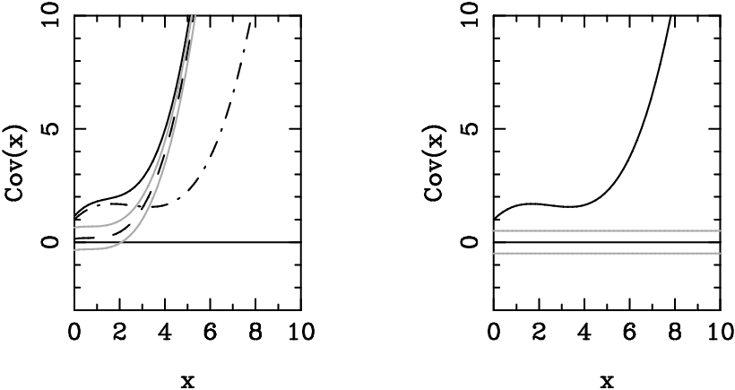
Furthermore there is some tolerance envelope around the systematic (gray solid lines) which represents the state of knowledge regarding the systematic. One can then subtract the mean and from the observable which results in an estimator of the signal
| (2) |
plus some residual systematic which is centered around zero. In general throughout we always consider the case that there is some extra data that places constraints on the systematic . This is shown in the right panel of Fig. 1, the systematic tolerance envelope now lies about the line.
The measurement of this signal to estimate the values of some parameters within a theory can be done in the usual way
| (3) |
where is the error on the signal. Note that we will remove (e.g ) from all equations for clarity. A best estimator of the parameters from the observation is defined such that . However this statistic has not taken into account the residual systematic effect in any way.
To make predictive statements regarding parameter estimation it is convenient to work with the Fisher matrix formalism. The Fisher matrix allows for the prediction of parameter errors given a specific experimental design and method for extracting parameters. In the case of Gaussian-distributed data where we assume that the error on the signal is not a function of parameter values we can take the covariance of the estimated values of the parameters (Tegmark, Taylor & Heavens, 1997; Jungman et al., 1996; Fisher, 1935)
| (4) |
where the Fisher matrix is defined by (Tegmark, Taylor & Heavens, 1997; Jungman et al., 1996; Fisher, 1935)
| (5) |
The marginal errors on the parameters are given by , this is the minimum marginal error that one can expect for the experimental design considered (due to the Cramer-Rao inequality; Tegmark, Taylor & Heavens, 1997).
| Approach | Broadens Likelihood | Bias Likelihood | Problems |
|---|---|---|---|
| Marginalise | Choice of parameterisation | ||
| Bias Formalism | Need to assess all allowed functions |
3.1 Model Fitting and Marginalisation
The marginalisation approach fits a model to the residual systematic and treats the systematic as an extra statistical effect. The model chosen for the systematic depends on a suite of new parameters and on the original parameter set where the total parameter set is given by . The extra parameters are then assumed to be part of the signal of a method. To estimate the values of the parameters the statistic of equation (3) is modified to
| (6) |
where the total is minimised to find the best estimator of the parameters. The likelihood functions for the cosmological parameters are found by marginalising the combined likelihood over the new parameters
| (7) |
The new Fisher matrix for the total parameter set becomes a combination of the cosmological Fisher matrix , the derivatives of the likelihood with respect to the cosmological parameters and the systematic parameters and the systematic parameters with themselves
| (8) |
Where the individual terms are given by
| (9) | |||||
here we have assumed that the errors are uncorrelated and do not depend on the parameters.
The predicted cosmological parameter errors now including the effect of the systematic are given by (see Appendix A for a more detailed expression). The cosmological parameter errors are increased due to the degeneracy between the cosmological and systematic parameters (included by the terms). The tolerance envelope around the residual systematic (Fig. 1) acts as a prior on the systematic parameters in the chosen model.
3.2 The Bias Formalism
The bias formalism treats a systematic as such, by not statistically marginalising over any extra parameters within a model. Instead the systematic simply adds an extra systematic function to the signal. By doing this a bias is introduced in the maximum likelihood value of the parameters with respect to the true underlying values
| (10) |
When marginalising the choice lies in the suite of parameters, and the function, chosen. Here there is a similar choice, one must assume that the systematic has some functional form . To estimate the values of the cosmological parameters , the statistic of equation (3) is modified to include the assumed systematic
| (11) |
The estimate of the parameter values will now be biased but the marginal error on the parameters will remain the same (the caveat here that this is only the case when the systematic is smaller than the signal).
It can be shown (Taylor et al., 2007; Amara & Refregier, 2007b; Kim et al., 2004) that, with the assumption of Gaussian likelihoods, the predicted bias in a parameter due to an uncorrected systematic is given by
| (12) |
where
| (13) |
To recap Sections 2 and 3, Table 1 summarises the effect on the likelihood surface and the primary problem encountered by each systematic approach.
In cases where the systematic affects the error on the signal (which is almost always) then leaving a systematic in the signal can cause a bias and increase the marginal errors. However the increase in marginal errors is negligible for systematics that have an amplitude which is much less than the signal, and cause biases that are (Amara & Refregier, 2007). Equation (12) is also an approximation for the case of small biases, if the bias is large relative to the marginal error then the curvature of the likelihood surface will have varied substantially from the Gaussian approximation. In such cases one could go to a higher order in the Taylor expansion used to derive equation (12), or calculate the full likelihood.
3.3 A Simple Example
To review the general formalism described thus far, and for use in subsequent Sections, we will here introduce a simple model. The toy model we will consider is shown in the right hand panel of Fig. 1. Referring to equation (1) the signal is given by a simple polynomial expansion
| (14) |
where the statistical parameters we are concerned with (with fiducial, true, values) are the parameters and . We assume that the observed signal is measured with an error of . We include the and terms so that the problem is slighly more realistic, in that there is an extra behaviour in the signal that we do not wish to constrain but may effect the determination of the parameters of interest.
Fig. 2 shows the simple model signal with some Gaussian distributed data points. We then calculate the two-parameter marginal errors using equation (3) where we use the model as in equation (14). Table 2 shows the measured marginal errors from this simple mock data, and compares these with the expected marginal errors calculated using the Fisher matrix (equation 5).
We then introduce a simple systematic into the model by assuming a simple function (note this does not have a mean of zero, but could fit into some boundary centered on )
| (15) |
By recalculating the likelihood and including this systematic function, using equation (11), we find that the most likely value of and is biased and yet the marginal errors remain the same. We compare this bias to the prediction made using equation (12) in Table 2.

| No Systematics | ||
|---|---|---|
| Parameter | Measured Error | Expected Error |
| Bias Method | ||
| Parameter | Measured Bias | Expected Bias |
| Marginalising Method | ||
| Parameter | Measured Error | Expected Error |
To test the method of marginalising over data we now reset the systematic (throw away equation, 15) and introduce a simple systematic which is measured using some mock data. Fig. 3 shows the model signal with some extra systematic data with a mean of zero and a scatter of . We then introduce a simple systematic model parameterised by a new parameter
| (16) |
and fit the model (equation 14) and the systematic to the data simultaneously, as described in equation (6). The total likelihood is then marginalised over . Fig. 3 shows that when this extra systematic is marginalised over the constraint on is affected the most since has the same functional form as this parameter, and so there exists a large degeneracy between and . The exact degeneracy is broken by the extra data available for the systematic. In Table 2 we show the increase in the marginal error on the parameters and when we marginalise over the extra systematic parameter .

We have now introduced the basic formalism and shown that this can be applied to a simple example that yields results which are in good agreement with the Fisher matrix predictions.
4 Form Filling Functions
For the remainder of this article we will present an alternative to marginalisation by advocating the bias formalism for dealing with systematics, outlined in Section 3.2. The issue with which one is now faced is what function to choose for the residual systematic. To investigate the full extent of possible biases, allowed by the tolerance on the systematic, all allowed functions must be addressed in some way.
In Fig. 4 we use an extension of the simple model, outlined in Section 3.3, to introduce the concept of two different forms of systematic tolerance. The tolerance envelope could have a hard boundary (e.g. defined by a theory which states that “the systematic must lie within this boundary”). Or the systematic could be defined by some extra data that has partially measured the magnitude of the systematic. We will refer to these two scenarios as the “hard bound” and “data bound” respectively.


To fully assess the level of bias every functional form allowed by the systematic tolerance envelope needs to be tested. For the hard boundary we want to find every function that can be drawn within the hard boundary. For the data bound every function can be weighted with respect to the data itself. Here we introduce the concept of ‘form filling functions’ which are a set of functions that should exhaustively fill the space of possible functions allowed by some tolerance envelope.
Consider the hard bound in Fig. 4, in the bias approach we want to find every function that will fit within this tolerance envelope. To do this we consider functions in the most general form as expansions in some arbitrary basis set
| (17) |
where , and and form some arbitrary basis functions. To choose the basis set we impose the following conditions
- •
The basis set must be complete in the range of we are considering i.e. all functions must be expressible as an expansion in the basis.
- •
The basis functions must be orthogonal.
- •
The functions must be boundable i.e. the basis set must be able to be manipulated such that every function described within some bounded region (tolerance envelope) can be drawn.
The first condition is necessary. The second condition is make some calculations more straightforward though is not strictly necessary. The third condition is merely desirable -- one can imagine having a basis set in which non-bounded functions are allowed, but when using such expansions one would have remove these stray functions. As an aside we note that over-completeness is not a problem as long as the basis set is in fact complete (we do not care if we sample a function multiple times, as long as we sample it at least once)11 1 Orthogonal basis sets are never over-complete so the second condition means we shouldn’t be in this situation for our functional form filling algorithm..
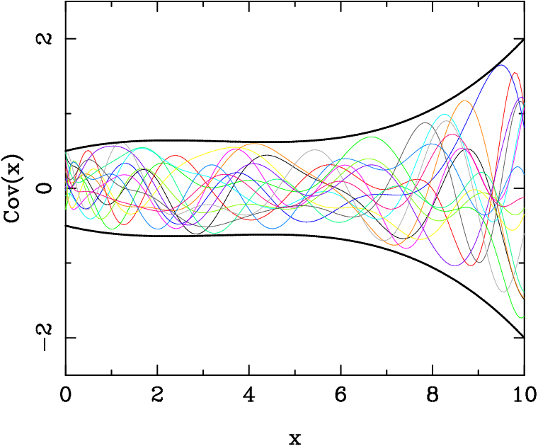


Algorithm. Equation (17) represents every function, however we are only concerned here with defining all functions within some bounded region. To begin we will show how an interval can be defined such that every function between can be drawn. For an orthonormal basis set the coefficients needed to draw a function can be expressed as
| (18) |
where is some interval over which the basis set is complete and is a weight function upon which the basis set is complete the constant ( is a diagonal) is calulated in general using
| (19) |
for all the basis sets we consider . Now we can write a general expression that provides a limit on . Using the triangle inequality we can write
| (20) |
and given that we have an expression for
| (21) |
So using equation (17) and limiting the coefficient values to (and similarly for ) every function with the region can be drawn22 2 Equation (21) is strictly only true for Riemann integrable functions, however essentially all bounded functions satisfy this constraint – in particular all class (smooth) functions, and all step functions. Examples of the type of (very peculiar) function that are not Riemann integrable are Dirichlet’s function and the Smith-Volterra-Cantor set..
We now define an arbitrary ‘bound function’ which describes a hard boundary (in Fig. 4 for example) where at any given point in the systematic functional form must lie in the region . Equation (17) is simply modified to include this arbitrary boundary
| (22) |
Now, if the basis set is complete, and (similar for ) equation (22) represents every possible function that can be drawn within the hard bound – and each function could yield a different bias. Note however that this statement says nothing about the probability that a particular function will be drawn.
An important caveat to this is that the total set of functions drawn using this algorithm is not bounded only some subset of the functions is. However a ‘clean’ subset of functions with can easily be drawn by removing any function for which at any .
In practice where the task of drawing all possible functions becomes a numerical/computational problem. For a given basis set the fundamental quantities that describe each and every function are the coefficients and . The task then is to explore the coefficient parameter space in an exhaustive a manner as possible.
As a first attempt the approach taken in this article is to randomly and uniformly sample the coefficient space , …, for . The free parameters in this approach, given a basis set, are the maximum order investigated and the number of random samples in the space that are chosen. We leave a more sophisticated Monte-Carlo formulation of this problem for future work.
When truncating the series we will be missing some highly oscillatory
functions (for the basis sets
considered) but we show in Appendix B that one can always make a definitive
statement about the fraction of all functional behaviour sampled down to some scale.
These free-form functions are regularised by the truncation of the basis set
and by the bound function.
Throughout the remainder of this Section we use the numerical
order and function number investigated in Appendix B.
Basis Sets. Throughout we will principally consider three different basis sets. These are
- •
Chebyshev polynomials . These functions form a complete basis set for , and are bounded by the region . To map these functions onto an arbitrary -range a variable transformation can be applied such that
(23) and for all .
- •
Fourier series. The Fourier series is a complete basis set in the range and the functions are bounded in the region for the basis set
(24) The cosine or sine of a real number are and .
- •
Tophat functions (binning). This uses a tophat functional form and is meant to be analogous to binning the -range. The maximum order in equation (17) here refers to the number of bins where for the bin is either zero or one depending on whether lies within the bin
(25) where and is the bin width. for all .
Table 3 summarises some of the basis set properties including the coefficient intervals over which a complete (sub)set of functions with can be drawn.
| Basis Set | Basis Functions | Orthogonal Weight | Orthogonal Constant | Interval | Coefficient Interval |
|---|---|---|---|---|---|
| Chebyshev | for ; for | for ; for | |||
| Fourier | for , & | for ; for | |||
| Tophat | H(-)+H(+) |
One may be concerned that there will always be some at which a boundary-touching function cannot be drawn. For every finite maximum index in the sum of equation (22), one can find a value of in such that cannot be at . The key realisation that we stress here is that this is a actually a statement about the scale upon which the space of functions is complete. The larger the maximum order , the smaller one can find an with for some , i.e. the concern is reduced to an issue of resolution because if then every function complete down to some scale can be drawn. We show this in Appendix B.
4.1 Hard Bound
Fig. 5 shows an example of a hard boundary and a random assortment of functions (a random, uniform, sampling of , …, ; and , …, for the Fourier basis set) for the Chebyshev, Fourier and tophat basis sets. As the order and number of functions is increased the functional forms begin to completely fill in the bounded area (hence “form filling functions”).
It can be seen even at this stage that the tophat basis set is not efficient at filling the bounded area. This is investigated further in Appendix B where we show that whilst all of the basis sets considered can fill any desired bounded region the Chebyshev and Fourier basis are many orders of magnitude more efficient in terms of computational time than the tophat functions (binning); we discuss computational time in Appendix C. This is a result of the restrictive step-like nature of the functions that binning imposes requiring a high order (number of bins) to characterise particular (smooth) functional behaviour. In addition to being inefficient, the tophat basis is not differentiable at the bin boundaries and as such could be construed as being un-physical, although in some special circumstances (e.g. photometric redshifts where a filter may have a tophat function in wavelength) a tophat basis set may be needed.
The key feature of the hard bound is that within the boundary all functions are given equal weight i.e. the probability that any given function is the ‘true’ systematic functional form is the same for all functions. Out of the full range of possible biases given a hard boundary, there should exist a maximum bias – because the space of functions and hence the range of biases is limited. We show that this is the case in Appendix D. The quantity of interest is therefore this maximum bias that is allowed by the functions that can be drawn within the hard boundary. In the data boundary case, Section 4.2, there is a maximum bias for each subset of functions that give the same weight (with respect to the data).
One intuitively expects that the systematic function that introduces the largest bias should be the one that most closely matches the signal term containing each parameter. In the case where there are degeneracies between parameters the worst function is some combination of the signals sensitivity to the parameters. Here we will use the simple example hard bound from Section 3.3 to demonstrate that in this case a maximum bias exists, and that this maximum is stable with respect to basis set.
Fig. 6 shows the maximum bias on as a function of the number of random realisations of the coefficient space for the Chebyshev, Fourier and tophat systematic basis sets, for all sets we consider a maximum order of . It can be seen that as soon as the “worst function” is found the maximum bias becomes constant and stable for the Chebyshev and Fourier basis sets. In this case the worst function is simply since this is the function that affects the signal () the most through the effect on (the worst function is a linear combination of the response of each individual parameter in the marginalised case, see Appendix D). There is an exact degeneracy since a function of the form will cause a bias of equal magnitude but opposite sign to , so in this case will also cause the same absolute bias (see Appendix D). For the top hat basis set it is very unlikely to find this particular worst function so the bias does not find the maximum even after realisations. The Chebyshev basis set finds this function after only a few realisations since is one of the basis functions of the Chebyshev expansion.
Fig. 6 is meant simply as an example of the type of convergence test that could be performed given a realistic application. In Appendix B we outline a diagnostic mechanism that can gauge whether a bounded area has been completely filled with functions.

4.2 Data Bound
If the systematic has been partially measured using data then there is no hard boundary within which all functions must lie, and every function is still allowed to some degree. The issue which must be addressed in this case is how each function should be weighted given the data available – a function is more likely to be the ‘true’ systematic signal if it is a good fit to the systematic data.
For the case of a data bound we propose a similar approach to the hard bound. We want to explore all possible functions, to do this we express an arbitrary function using an expansion as in equation (22). By choosing a complete basis set (e.g. Chebyshev, Fourier) the full space of functions can be explored by exhaustively exploring the space of coefficients, as described in Section 4.1.
In the following we will concatenate the two basis sets and for clarity, however note that for the Fourier basis set two sets of coefficients are needed.
The critical difference in this case is that for each function that is drawn we can assign a weight using the statistic
| (26) |
This quantifies how good a fit the function (the values of and , and some basis set) is to the residual systematic data.
However since we aim to exhaustively try every function (complete down to some scale) there will exist some functions that fit exactly through the data points. This causes a problem when using the statistic as a weight for such functions will have a , and hence be given a probability that such a function is likely, but such a conclusion has not taken account of the error bars on the systematic data.
In this simple example we have subtracted the mean of the systematic signal so data should be scattered about . In the case of Gaussian distributed data the scatter of the data points should be proportional to the error bar on each data point. If the observation could be repeated then the data points would be scattered in the same statistical manner about but have different actual values. This is very similar to the familiar sample variance; in cosmology we are used to a special kind of sample variance that we call cosmic variance in which the likelihood of the data, given only one realisation of our Universe, must be taken into account.
To take into account this sample variance effect we must consider the likelihood of the residual data. In Appendix E we show how for Gaussian distributed data the probability of a function , given some set of observations, can be written as a sum over , where at each point there is some data with an error bar as
| (27) | |||||
where we have translated the notation of equation (105) to reflect that of equation (26). For any given set of data the second term in equation (27) is a benign additive constant so the weight that we assign each function is
| (28) |
We stress that this is for Gaussian data with a known mean of zero such a function is uniquely described by the variance.
In general data may not be exactly centered at zero or be Gaussian distributed. As an alternative to the analytic procedure of marginalising over the data one could create Monte-Carlo realisations. For each realisation one could measure the of the fit of a given function to the data from equation (26) and assign a weight as the average over all realisations
| (29) |
where the extra factor of converts the average to a log-likelihood similar to equation (28).
The bound function in equation (22) represents a hard prior in this case. One should choose a bound function is much larger than the scatter in the systematic data . Any functions that deviate from the data by a large amount will be down-weighted by the poor fit even though they may yield a large bias, so as long as the boundary within which functions are considered is away from the data then any results should be robust.
For each function one now has an associated bias and a weight. Now consider a particular bias in some parameter: there exists a set of systematic functions that could yield this same bias and from that set there must exist a function which is the best fit to the data. If each best-fitting function for every bias can be found then one is left with a robust weight for each bias and a measure of the relative probability allowed by the data
| (30) |
is the minimum weight (equation 28) from the space of functions defined by the coefficients that yields the bias .
Another way of putting this is that for a given weight there exists a maximum and minimum bias. We show in Appendix D that, within the Fisher matrix approximation of equation (12), that there does indeed exist a maximum and minimum bias for each weight.


Fig. 7 shows the weight (equation 28) for each function drawn from the Chebyshev, Fourier and tophat basis sets against the bias induced by the function using the data bound toy model of Fig. 4. It can be seen from this Figure that for any given bias there exists a minimum weight that can be achieved by the functions giving that bias. In the right bottom panel of Fig. 7 we have found the minimum weight for each bias and converted this into a likelihood using equation (30) showing that this procedure is robust to the choice of basis set used (though the tophat basis set is far less efficient than Chebyshev and Fourier, see Appendix B for more details).
One can of course extend the formalism introduced here to an arbitrary number of dimensions. To extend this to two dimensions we have modified the simple example to have a much smaller data bound, since (as can be seen in Fig. 7) the fiducial scatter in the toy model systematic data introduces large biases in the measured parameters. Fig. 8 shows the joint statistical constraint on and for the mock data shown. On this same plot we show the systematic contours from the residual systematic – within the systematic contour there is a probability that the statistical maximum likelihood is biased.
We again show results for two different basis sets and show that the systematic contours are again independent of the basis set chosen. We have not used the tophat basis because it is not an efficient basis set (in terms of computational time, see Appendix B) to use even for a one dimensional analysis.
In a real application one would hope to show such plots with the systematic contours lying within the statistical ones, but for illustrative purposes we have shown a dominant systematic here. A hard bound in this case would represent a tophat contour in probability where, within the contour, the probability equals unity and outside the contour the probability is zero.

In the marginalisation approach one could also draw two sets of contours, but both would be statistical: one that has no systematic and the other in which a systematic has been included. Fig. 8 represents one of the key recommendations of this article, that in future we must not only show statistical contours for cosmological parameters but also systematic probability contours. Here we have shown one way of obtaining a robust estimate of such systematic probability contours.
4.3 Marginalisation vs. Bias
The bias and the marginal error are inter-related via the mean square error (MSE) which is defined, for a parameter , as
| (31) |
where is the marginal error on and is the bias. So both marginalisation over systematic parameters and functional form filling increase the MSE through the marginal error and bias respectively.
In Appendix A we show that the marginalising approach and the functional form filling approach are different however there is a subtelty. If the parameterisation and order are the same (i.e. a truncated basis set is used) then the MSE recovered from marginalising or considering the bias is the same. The conclusions from Appendix A are
- •
If the functional form of the systematic is known then the degradation in the MSE as a result of marginalising or functional form filling (bias) is the same.
- •
If the functional form of the systematic is unknown then the MSE from marginalising will tend to underestimate the true systematic error and is in general not equal to the MSE from functional form filling.
- •
Given that the marginalising necessarily truncates the basis set there are always some functions that marginalising cannot assess.


Given that the MSE, given a particular functional subset is the same for bias and marginalisation the key difference between marginalisation and functional form filling is that in marginalisation case the functional space is truncated by the choice of parameterisation and ultimately by the number of data points.
Looking back at Fig. 7 the functional form filling technique fills out the Weight–MSE (bias) bounded region by sampling every function down to some scale. To illustrate the way in which marginalisation cannot sample the full space of functions we have reproduced these plots but using various truncated basis sets. Note that the MSE from the bias and marginalisation is the same given a parameterisation as shown in Appendix A – marginalising is like functional form filling but with a very restricted class of function.
Fig. 9 shows the weight (fit to data) vs. bias using
the simple toy model for
the Chebyshev and Fourier truncated basis sets for realisations
of each truncated set. We truncate the
expansion at , and . It can be seen that if is used
the space of functions is very restricted, and as the order is
increased the space of functions increases. These results are also in
resonance with Appedix B. If one were marginalising a choice of
parameterisation (basis and order) would have to made in which case
the MSE conclusion would be dependent on this choice.
Discussion
We take this opportunity to discuss the difference between marginalising and functional form filling. Functional form filling is not the same as marginalising over a very large parameter set on a qualtitative level: we are not finding the best fit values of the parameters but rather using each parameter combination simply as a prescription that yields a particular bias. As the freedom in the functions increases (more parameters) the functional form filling approaches a stable regime in the results it gives. Functional form filling yields the probability that the maximum likelihood value is biased by some amount, whereas marginalisation yields a probability that the cosmological parameters take some value jointly with some values of the nuisance parameters.
One could marginalise over a very large number of parameters but in this case the joint covariance matrix will at some point necessarily become computationally singular as parameters are introduced can cannot be constrained by the data. One way to consistently include more parameters than data points is to add a prior such that any extra parameters were constrained where ansd ; but this requires adding the prior on which requires justification.
In the lack of any external prior the number of parameters that can be used in marginalising is necessarily truncated at a low order since once the number of free parameters becomes larger than the number of data points (for the data bound) the parameter fitting methodology becomes ill-posed (e.g. Sivia, 1996). In contrast the functional form filling technique could use an infinite basis set expansion (only computational, and physical, resources prohibit this) since we use the basis set simply as a prescription for drawing functions through the systematic – one could even draw these by hand if you were sure that you could draw a complete set of functions.
One may be concerned that information is being ignored or disgarded. Quite the opposite from discarding information present in data we assign a weight to every possible function with respect to the data, in this sense we throw nothing away – every function has a weight and a bias. In constrast when marginalising the functional space assessed is limited by the number of data points and as such a very large class of functions are never considered – if a basis set is truncated these are usually highly oscillatory functions.
The bias formalism becomes preferable if there is uncertainty over what the functional form is (which is most, if not all of the time).
In Appendix A we show that for the same basis set and prior functional form filling and marginalisation produce the same results in a mean-square-error sense. Hence in the limit of marginalising over functions, with suitable priors, the two approaches should produce the same results – in this article we focus on bias functional form filling.
4.4 Summary
We have presented an alogorithm by which any function within a bounded region can be drawn this is summarised as
- •
Chose a complete orthogonal basis set. We recommend Chebyshev polynomials because of their ease of calculation and computational efficiency (see Appendix B).
- •
Use equation (21) to calculate the interval over which the coefficient must be sampled.
- •
Define the bounded region within which functions must be drawn.
- •
Define a scale upon which the functional space must be complete.
- •
Randomly and uniformly sample from the space of coefficients using a maximum order and number of realisations such that the functional space is fully filled – the diagnostic tools from Appendix B can be used to guage the level of completness.
By defining the hard and data bounds we have now presented all the tools needed to correctly assess a systematic given some prior knowledge of the magnitude of the effect, either an external data set or some theoretical knowledge. In the hard boundary case every function is given equal weight and as such a maximum bias should exist. In the data boundary case a probability can be assigned to each bias.
We emphasise here that this method requires there to be at least some information at every data point associated with the signal – either a hard boundary or some systematic data. If there were no constraint the ranges of biases could become unbounded.
Our proposal is that when measuring some cosmological parameters these techniques can be used to augment the statistical marginal error contours: some cosmological parameters are measured and about their maximum likelihood point are drawn some marginalised statistical error contours and in addition:
- •
If a theory or simulation provides a hard boundary to some systematic then the maximum bias will define a systematic contour that can be drawn in within which the maximum likelihood could be biased.
- •
If some data is provided that measures the systematic then a further set of systematic contours can be drawn which will show the probability that the maximum likelihood point is biased by any particular amount.
The goal for any experiment is to control systematic effects to such a degree that any systematic contours drawn are smaller than the statistical contours.
We will use the functional form filling approach in the next Section to place requirements on weak lensing systematics. For general conclusions please skip to Section 6.
5 An Application to Cosmic Shear Systematics
We will now use the functional form filling approach to address shape measurement systematics in cosmic shear (due to methods Heymans et al, 2006, Massey et al., 2007; or PSF inaccuracies Paulin-Henriksson et al., 2008; Hoekstra, 2004). This Section represents an extension of the work of Amara & Refregier (2007b) where certain particular functional forms were investigated. Here we extend the analysis to include all functional behaviour to fully address the impact of the systematic. For a thorough exposition of cosmic shear we encourage the reader to refer to these extensive and recent reviews and websites (Munshi et al., 2006; Bartelmann & Schneider, 2001; Wittman, 2002; Refregier, 2003; http://www.gravitationallensing.net). The source code related to the work in this Section is released through http://www.icosmo.org, see Appendix F for details.
5.1 Background
Cosmic shear tomography uses both the redshift of a galaxy and the gravitational lensing distortion, shear, to constrain cosmological parameters. The observable in this case is the lensing power spectrum as a function as redshift and scale . Since we have redshift information the galaxy population is split into redshift bins where each bin has its own auto-correlation function and the cross-correlations between bins are also be taken.
Throughout this Section we will use a fiducial cosmology of , , , , , , , where we parameterised the dark energy equation of state using (Chevallier & Polarski, 2001; Linder, 2003) and included the spectral index , we consider non-flat models throughout where . We assume a weak lensing survey (similar to the DUNE/Euclid proposal, Refregier et al., 2008a) which has an Area square degrees, a median redshift of (using the given in Amara & Refregier, 2007b) with a surface number density of galaxies per square arcminute. We also assume a photometric redshift error of and split the redshift range into tomographic bins.
The observed lensing power spectrum can be written as a sum of signal, systematic and noise terms
| (32) |
so that an estimator of the observed lensing power spectrum can be written by subtracting the shot noise term
| (33) |
where is the underlying true lensing power spectrum, dependant on cosmology, which we want to measure and is some residual systematic. The error on this estimator can be written as
| (34) |
note that this is the error on the observed signal, not the observed signal itself, so that as the systematic increases the error on the observed increases. The Fisher matrix and bias are then defined in the usual way (equations 5 and 12) where .
| Parameter | Marginal Error |
|---|---|
Table 4 shows the expected marginal errors on the cosmological parameters using the fiducial survey calculated using the Fisher matrix formalism, note that no prior has been added to these results, they are for lensing alone.
The additive systematic which we consider here is a special kind that has the same shape as the lensing power spectrum but where it is multiplied by some unknown systematic function (sometimes referred to as a multiplicative systematic) (we use the notation of Amara & Refregier, 2008b)
| (35) |
where means the correlation between redshift bins and , an auto-correlation is where . The particular form of multiplicative bias we consider is that which causes the true shear, as function of angle and redshift , to be incorrectly determined such that the residual systematic shear is related to the true shear by some function
| (36) |
So that the systematic given in equation (35) can be written . This expression from Amara & Refregier (2007b) actually assigns an to each redshift slice where each is the bin weighted average. A more accurate approach is to include in the integrand of the lensing kernel ( in Appendix A of Amara & Refregier, 2007b). We compared results when the bin-weighted average was used against the correct integral method and found exact agreement, this is because the bins are narrow and the functional variation on sub-bin width scales is small.
We note that Huterer et al. (2006) have used Chebyshev polynomials in weak lensing systematic analysis, although they marginalise over a systematic parameterised using Chebyshev polynomials and then investigate the biases introduced if the most likely value of the estimated coefficients were incorrect. Here we are not measuring the Chebyshev coefficients but rather using this basis set to draw every possible function and determine the bias introduced by the function itself not some misestimation of any particular coefficient. The approach outlined in this article also has a resonance with the work of Bernstien (2008) in which flexible basis sets are used to address systematic quantities, although this is done within the self-calibration (marginalising) framework, and their general thesis is that of tuning the models that are marginalised over. Bernstien (2008) notes that an approach such as the one outlined in this article, using the formalism of Amara & Refregier (2007b), would be desirable in certain situations.
5.2 Functional Form Filling for m(z)
We will now place constraints on the function such that that the measurement of the cosmological parameters are robust. We first define some boundary (bound function) on such that any systematic function must lie within the bounded region. We parameterise the hard boundary (Section 4.1) using
| (37) |
we want to know what values of and are sufficient to ensure that the bias on cosmological parameters are less than their statistical error ; . We stress that this is a parameterisation of the boundary within which a function must lie, not the function itself.
To fill the bounded area with every functional form, complete down to the scale of , we use Chebyshev polynomials with a maximum order of and investigate realisations of the basis set, using the formalism outlined in Section 4. We do not expect any of the cosmological parameters to introduce features into the lensing power spectrum on scales so this should be sufficient.


Fig. 10 uses the diagnostic measure described in Appendix B to show that on the scale of every possible functional behaviour has been experienced at every point within the bounded region, for this example we use and .
To begin we will first consider with and . Using the functional form filling technique we have identified which systematic functions cause the largest bias for each cosmological parameter. Table 5 shows the maximum bias to marginal error ratio for each cosmological parameter due to this particular .
We have taken into account all degeneracies between parameters in this exercise – in the terminology of equation (12) the inverse Fisher matrix is marginalised over all parameters and the takes into account degeneracies between the cosmology and systematic functions.
| Parameter | bias/marginal error |
|---|---|

Fig. 11 shows the worst functions, that cause the largest bias, for each cosmological parameter. Since there are degeneracies between all parameters the worst function is practically the same for all parameters.
We find that the ratio of the maximum bias to the marginal error is for most parameters, except which is is not acceptable: the bias is larger than the statistical error. These results are in rough agreement with Amara & Refregier (2007b) where it was concluded, with a restricted functional parameterisation of , and the assumption of a flat Universe, that and yielded biases that were but were somewhat on the limit of what is acceptable. Furthermore it was concluded that functions which have a variation (cross from positive to negative) about have the largest effect, we also find that the functions that cause the largest bias in all the parameters varies in the region of . This is because it is at that dark energy begins to dominate and so the parameters and , and through degeneracies the other parameters, are affected by systematic functions that introduce variation at this redshift.
Fig. 12 shows the ratio of bias to marginal error as a function of and for . It can be seen that the redshift scaling has the expected effect on the maximum systematic bias: as increases the maximum bias for a given also increases as the systematic bounded area expands. The solid lines in Fig. 12 show the contours. For we need a for the bias on to be acceptable. If the redshift scaling is eliminated then the requirement on the absolute magnitude of is relaxed to .


Fig. 13 shows the affect of survey area on the requirement of and . The lines in this figure show the contours for varying survey area. We have picked as an example since this parameter provides the most stringent constraints on the shape measurement parameters (see Table 5 and Fig. 12). As the survey area increases and the marginal error on decreases the requirement on shape measurement accuracy becomes more stringent. We have fitted a simple scaling relation to these contours so that for statistical errors to be reliable the following relation holds
| (38) |
The requirements on and for the largest survey considered are at the limit of currently available shape measurement techniques, that yield on average at best (Miller et al, 2008; Kitching et al., 2008b). A large redshift variation of results in large biases (Fig. 11) so a shape measurement method that is unaffected by the magnitude/size of the galaxy population should yield robust cosmological constraints. For example Kitching et al. (2008b) have shown that the lensfit method has a characteristic that has a small magnitude/size dependence. In this case, , and a more relaxed constraint on – is required which is well within reach of these most recent developments in shape measurement. These results are also in agreement with Semboloni et al. (2008) where they find that for a very restrictive class of functions, of the form , but a more complex likelihood description, that some parameter combinations of and can give rise to biases that are less that the cosmological errors.
For the smaller surveys considered, that are well matched to currently available or upcoming experiments (e.g. CFHTLS, van Waerbeke et al., 2001; Pan-Starrs, Kaiser, 2002), the shape measurement techniques currently available have biases (Heymans et al., 2006; Massey et al., 2007; Kitching et al., 2008b) that are well within the required level of accuracy. The caveat to these conclusions is that here we have not discussed the size or galaxy-type dependence of any bias and we have not considered any calibration offset in the measured shear.
6 Conclusion
In this article we have presented a method that allows one to move beyond the tendency to treat a systematic effect as a statistical one. When a systematic is treated as a statistical signal extra parameters are introduced to describe the effect, and then these extra nuisance parameters are marginalised over jointly with cosmological parameters. We have shown that even in a very simple toy model such an approach is risky at best. The results being highly dependent on the choice of parameterisation, and in the limit of a large number of parameters any statistical signal on cosmological parameters can be completely diluted. One could use marginalisation if there exists a compelling physical theory for the systematic, however if the functional form is merely phenomenological or if it contains a truncated expansion then one should use caution. Even in the case that confidence is high with respect to the assumed functional form any residual must be investigated correctly.
As an alternative we advocate treating a systematic signal as such, an unknown contaminant in the data. We address the situation where we have at least some extra information on the systematic, either from some theory or simulation that may provide a hard boundary within which a systematic must lie, or from some external data set. We leave the case of ‘entangled systematics’ (where there is no extra information and where the systematic depends on the cosmological parameters) to be investigated in Amara et al. (in prep). Throughout we have introduced each concept using a simple toy model.
Since the systematic is treated as a genuine unknown we must address every possible functional form that is allowed, by either the hard boundary or the extra systematic data. To do this we use complete basis sets and randomly sample from the space of coefficients until all functional behaviour has been experienced at every point with the hard boundary, or within a few of the data. We have shown that such “functional form filling” can be achieved by this technique using either Chebyshev, Fourier or tophat basis sets. By treating each function as a possible systematic, a bias in the maximum likelihood value is introduced whilst the marginal error stays the same. Throughout we have shown that as long as functional filling is achieved all conclusions on the magnitude of a systematic effect are independent of the choice of complete basis set – though binning is highly inefficient in terms of computational time, and could be labelled as an unphysical basis set.
For the case of a hard boundary every function is given an equal probability and as such a maximum bias exists. For the case of extra systematic data we show that a probability can be assigned to each function, and bias, allowing for the production of robust systematic probability contours.
We have made a first application of hard boundary functional form filling by addressing multiplicative systematics in cosmic shear tomography; we have left an application of the data bound for future work. We address a lensing systematic, that can result from shape measurement or PSF reconstruction inaccuracies, that has the same overall shape as the lensing power spectrum but is multiplied by some extra function. This is commonly represented using a multiplicative function (Heymans et al, 2006; Massey et al., 2007) where . For a DUNE/Euclid type survey, we find that in order for the systematic on to yield a bias smaller than the marginal error the overall magnitude of should be for a linear scaling in , but as the magnitude of the redshift scaling is relaxed then the requirement on increases to . The most recent shape measurement methods have (e.g. using the lensfit method Miller et al., 2007; Kitching et al., 2008b) and have a small scaling as a function of magnitude/size. The results shown here then, coupled with some currently available shape measurement techniques imply that constraints on cosmological parameters from tomographic weak lensing surveys should be robust to shape measurement systematics (with the caveat that PSF calibration and galaxy size dependence of the bias have been neglected here).
The techniques introduced here should have a wide application in cosmological parameter estimation: in any place in which there is some signal with some extra information on a systematic. For example baryon acoustic oscillations and galaxy bias, CMB and foregrounds, galaxy clusters and mass selection, supernovae and light rise times, weak lensing and photometric redshift uncertainties. A sophistication of these techniques could assign different weights/prior probabilities to particular functional forms, that are known a priori to have a large/small effect on cosmological parameter determination, such weights could come from either theoretical or instrumental constraints.
Cosmology is entering into a phase in which the statistical accuracy on parameters will be orders of magnitude smaller than anything achieved thus far. But we must take care of systematics in a rigorous way to be sure that our statistical constraints are valid. There exists the pervading worry that the functional forms used to parameterise systematics are not representative of the true underlying nature of the systematic and that something may have been missed. In such a scenario one should always add the warning that “cosmological constraints are subject to the assumption of the systematic form”.
Here we have presented a way to address systematics in a way that requires no external assumptions, allowing for robust and rigorous statements on systematics to be made.
Acknowledgments
TDK is supported by the Science and Technology Facilities Council, research grant number E001114. AA is supported by the Swiss Institute of Technology through a Zwicky Prize Fellowship. FBA is supported by an Early Careers Fellowship from The Leverhulme Foundation. BJ is supported by the Deutsche Telekom Stiftung and by the Bonn-Cologne Graduate School of Physics and Astronomy. We thank Andy Taylor for many detailed discussions on functional form filling. We thank the organisers and participants of the Intrinsic Alignments and Cosmic Shear Workshop at UCL on March – April 2008. In particular Sarah Bridle, Catherine Heymans, Rachel Mandelbaum, Lindsay King, Bjoern Schaefer and Oliver Hahn. We would also like to thank all members of the DUNE/Euclid weak lensing working group. We also thank Eric Linder, Lance Miller, Anais Rassat and a rigorous referee for many insightful discussions.
References
- [1] Albrecht, A. et al.; 2006, eprint arXiv:astro-ph/0609591
- [2] Amara A., Refregier A., 2007, MNRAS, 381, 1018
- [3] Amara A., Refregier A., 2007b, arXiv0710.5171
- [4] Amara A., Abdalla, F., Joachimi B., Kitching T. D., Refregier A., in prep.
- [5] Abazajian, K.; Dodelson, S.; 2003, PhRvL, 91, 1301
- [6] Ballinger W., Heavens A., Taylor A., 1995, MNRAS, 276, 59
- [7] Bartelmann M, Schneider P.; 2001, PhR, 340, 291
- [8] Bernstein, G.; 2008, arXiv0808.3400
- [9] Bridle, S.; Abdalla, F. B.; 2007, ApJ, 655, 1
- [10] Bridle, S.; King, L.; eprint arXiv:0705.0166
- [11] Brown, M. L.; Taylor, A. N.; Bacon, D. J.; Gray, M. E.; Dye, S.; Meisenheimer, K.; Wolf, C.; 2003, MNRAS, 341, 100
- [12] Catelan, P.; Kamionkowski, M.; Blandford, R.; 2001, MNRAS, 320, 7
- [13] Chevallier, M.; Polarski, D.; 2001, IJMPD, 10, 213
- [14] Cooray, A.; 1999, A&A, 348, 31
- [15] Crittenden, G.; Natarajan, P.; Pen, U.-L.; Theuns, T.; 2001, ApJ, 559, 552
- [16] Fisher, R.; 1935, JRoyStatSoc, 98, 35
- [17] Hannestad, S.; Wong Y.; 2007, JCAP, 07, 004
- [18] Heavens A.F., 2003, MNRAS, 343, 1327
- [19] Heavens A., Taylor A., 1995, MNRAS, 275, 483
- [20] Heavens A.F., Kitching T.D., Verde L., 2007, MNRAS, 380, 1029
- [21] Heavens, A. F.; Refregier, A.; Heymans, C.; 2000, MNRAS, 319, 649
- [22] Heymans, C., et al.; 2006, MNRAS, 368, 1323
- [23] Heymans, C.; Heavens, A. F.; 2003, MNRAS, 339, 711
- [24] Hirata, C.; Seljak, U.; 2004, PhRvD, 70, 3526
- [25] Hoekstra H.; 2004, MNRAS, 347, 1337
- [26] Hu W., 1999, ApJ, 522, 21
- [27] Hu W., 2002, Phys. Rev. D66, 3515
- [28] Huterer, D.; Masahiro, T.; Bernstein, G.; Jain, B., 2006, MNRAS, 366, 101
- [29] Huterer, D.; Masahiro, T.; 2005, APh, 23, 369
- [30] Jain B., Taylor A., 2003, Phys. Rev. Lett., 9, 1302
- [31] Joachimi, B.; Schneider, P.; 2008, arXiv0804.2292
- [32] Jungman, G.; Kamionkowski, M.; Kosowsky, A.; Spergel, D.; PRD, 54, 1332
- [33] Kaiser N., et al; 2002, SPIE, 4836, 154
- [34] King, L. J.; Schneider, P.; 2003, A&A, 398, 23
- [35] Kim A., et al., 2004, MNRAS, 347, 909
- [36] Kitching, T. D.; Taylor, A. N.; Heavens, A. F.; 2008a, MNRAS, 389, 173
- [37] Kitching, T. D.; Miller, L.; Heymans, C.; Heavens, A. F.; Van Waerbeke, L.; 2008b, MNRAS, 390, 149
- [38] Kitching, T. D,; Heavens, A. F.; Verde, L.; Serra, P.; Melchiorri, A; 2008c, Phys. Rev. D 77, 103008
- [39] Kitching, T. D,; Amara A.; Rassat R.; Refregier A.; 2008d, submitted to A&A
- [40] Kunz, M.; Sapone, D.; 2007, PhRvL, 98l1301
- [41] Linder, E.; 2003, Phys.Rev.Lett., 90, 091301
- [42] Massey R., et al.; 2007, MNRAS, 376, 13
- [43] Miller, L.; Kitching, T. D.; Heymans, C.; Heavens, A. F.; Van Waerbeke, L.; 2007, MNRAS, 382, 315
- [44] Paulin-Henriksson, S.; Amara, A.; Voigt, L.; Refregier, A.; Bridle, S. L.; 2008, A&A, 484, 67
- [45] Peacock, J.; Schneider, P.; 2006, Msngr, 125, 48
- [46] Pedersen K., Dahle H., 2007, ApJ, 667, 26
- [47] Percival W., et al., 2004, MNRAS, 353, 1201
- [48] Refregier A.; 2003, Ann.Rev.Astron.Astrophys, 41, 645-668
- [49] Refregier A., et al.; 2006, SPIE, 6265, 58
- [50] Refregier A., Douspis, M., et al.; 2008a, SPIE, 23 - 28 June
- [51] Refregier A.; Amara A.; Rassat R.; Kitching T.; 2008b, submitted to A&A
- [52] Semboloni E., Tereno I., Heymans C., van Waerbeke L., 2008, submitted to MNRAS
- [53] Seo H., Eisenstein D., 2003, ApJ, 598, 720
- [54] Sivia, D. A.; 1996, Oxford University Press, Clarendon Press
- [55] Starkman, G.; Trotta, R.; Vaudrevange, P.; 2008, arXiv0811.2415S
- [56] Tadros H. et al, 1995, MNRAS, 305, 527
- [57] Takada M., White M., 2004, ApJL, 601, 1
- [58] Taylor, A. N.; Kitching, T. D.; Bacon, D. J.; Heavens, A. F.; 2007, MNRAS, 374, 1377
- [59] Tegmark, M.; Taylor A., Heavens A.; 1997, ApJ, 440, 22
- [60] Wittman, D.; 2002, LNP, 608, 55
- [61] van Waerbeke, L.; et al.; 2001; cpgl, conf, 165
Appendix A : Marginalisation vs. Bias
Here we will show how marginalisation is mathematically different to the bias formalism used in the main article.
When marginalising the log-likelihood of some cosmological parameters can be written, for a signal some theory and a systematic as
| (39) |
When marginalising over the systematic the effect is parameterised by some extra parameters . If extra data is provided on the systematic then this adds a prior such that the total log-likelihood can be written
| (40) |
The Fisher matrix for this is created by taking the derivatives of the log-likelihood with respect to cosmological parameters and systematic parameters so that the first and second terms in equation (40) give the following Fisher matrices
The marginal error on the cosmological parameters is found by inverting equation (Appendix A : Marginalisation vs. Bias). The inverse of the upper left-hand segment of the Fisher matrix in equation (Appendix A : Marginalisation vs. Bias) can be found by using the Schur complement of the block matrix and then expanding this using the Woodbury matrix identity which gives
where , and . The marginal error in the case of no systematic () has been increased by an extra factor that depends on the degeneracies between the systematic parameters and the cosmological ones () and on the information available on the systematic parameters themselves (). This is also equal to the mean square error of the cosmological parameters in this case, since no bias is introduced.
For the bias functional form filling technique the log-likelihood of the cosmological parameters can again be written as
| (50) |
In the data bound case we can assign a weight to each systematic function (not extra parameters)
| (51) |
so that a very similar expression to equation (40) can be written for the joint log-likelihood of the cosmological parameters and the systematic
| (52) |
We have not necessarily parameterised with any parameters we wish to measure, can simply be a function that has been arbitrarily drawn through the systematic data. However if the systematic is parameterised (as we do in the functional form filling approach using complete basis sets) then the signal data is not used to determine the values of the extra parameters – the number of degrees of freedom in the fit has been reduced with respect to the marginalising case. The systematic data (or a hard boundary) is used to determine the probability of the systematic. Hence the Fisher matrix can be written, in this case, like
The inverse of the upper left-hand segment is now simply . Using the result from Appendix D (for the hard boundary case) a bias is introduced with a maximum value of
| (61) |
We have again condensed the notation so that . Note that . Hence the total mean-square error on cosmological parameters for the bias case comes from the unaffected marginal error of the cosmological parameter and the bias
| (62) |
a similar expression can be written for the data bound case, see Appendix D equation (99). We have compressed the subscript notation from equation (61) in equation (62).
These equations show how marginalisation and the bias formalism relate in a general sense, and that they are mathematically different objects i.e. when finding the maximum bias using the functional form filling approach the MSE between marginalisation and functional form filling can be different. This difference arises because the space of functions probed by marginalisation is restricted. In the next section we will show that if the functional space assessed is the same then the MSE should be equal.
Information Content
If the parameterisation, and number of (truncated) parameters, are the same then the MSE resulting from the bias or marginalising is the same. We show this here using a simple illustrative example.
We approximate the nuisance correlation as a first-order expansion of a set of parameters
| (63) |
This can be though of as a restricted set of functions or a special case of . The nuisance parameters will be correlated with the cosmological parameters and we can form the extended vector and Fisher matrix as shown in equation (Appendix A : Marginalisation vs. Bias), as in equation (Appendix A : Marginalisation vs. Bias) we can write the marginalised covariance matrix of like
| (64) | |||||
and there is no bias of the measured parameters. The subscript ‘c’ on the covariance indicates that we are including the covariance between and .
If instead we do not account for the covariance between and in the data, the measured error in the parameters is
| (65) |
but we have induced a bias in the measurement of ,
| (66) |
where is the variance of the data. Using our linear expansion of we find
| (67) |
From this can see the bias effect explicitly comes through the correlation of the nuisance parameters with the cosmological parameters, via .
We can simplify things further by considering a single parameter and a single nuisance parameter . The conditional error on the parameter can be simplified to
| (68) |
where we have introduced the correlation coefficient defined as,
| (69) |
We can see this by looking at the inverse of the matrix ;
| (70) |
The marginalized error on is
| (71) |
Similarly the marginalized error on is given by
| (72) |
Note that the marginalized errors on and go to infinity when the correlation coefficient is unity, . This is because and are completely degenerate.
From the definition of the correlation coefficient we can write the covariance between and as
| (73) |
which agrees with the definition of given in equation (69).
Note that the results for , and are not just the errors and covariance when we marginalize. They are also the errors and covariances when the parameter is correlated with . The only way to get back the uncorrelated errors is if and are uncorrelated, so , or if we know from some other measurement, in which case they effectively decorrelate. Even if we assume some value, or range of values, for , there is still a correlation between possible values of and .
Now consider the bias on , , when we ignore the nuisance effect (or assume some fixed form) . In our simple model the bias can be written
| (74) |
Now the error on the bias, including all the correlations between parameters, is given by
| (75) |
One might have mistakenly thought that the covariance between and was
| (76) |
but in doing so we have ignored the real correlation between and that exists. In the case that of fully correlated parameters, when , the error on is only the uncorrelated error on , whereas the real uncertainty is infinite.
Finally the correlation between the bias and the cosmological parameter is
| (77) |
Now we want to compare the effect of the bias with marginalization on the error of . In the case of marginalization this is given by the correlated covariance
| (78) |
In the case of bias, we have to add the uncorrelated error, , with the error in the bias value, , which does include the correlation between cosmological and nuisance parameters, to form the MSE;
| (79) | |||||
Hence the MSE is the same as the marginalized error in this simple case, and there is no loss or gain of information. Our result here is for a 2-parameter case, but is easily extended to multiple parameters.
It is worth thinking about the assumptions that lead to this result. For instance we have assumed in our analysis that the nuisance bias is completely specified by the parameter .
This shows that if one fully understands the nuisance effect, there is no difference between marginalisation and form-filling. Given marginalisation can be done quickly, and in some cases analytically, we would advocate marginalisation in this case.
However, if the form of the nuisance function is not known, or is wrong, marginalization will tend to underestimate the true systematic error because of the limited functional space explored by the set of functions assessed by the truncated basis set.
Given that in general the number of parameters that can be marginalised over is limited by the number of data points if the systematic parameterisation is unknown then the marginalising will necessarily not be able to assess the impact of some functions.
Constraining nuisance effects with external data
The effect of additional, external data to constrain the nuisance effects will add an extra Fisher matrix to ;
| (80) |
If we define a new parameter
| (81) |
as the ratio of the conditional error on from the original dataset to the expected measured accuracy on from the external data. If the error on from the external data is small, we can expect to be large, while of the external error is large, will be small. This results in the correlation coefficient becoming
| (82) |
When the error on the nuisance parameters is highly constrained by the new data set, and the correlation coefficient decreases. The effect of new data in the nuisance functions is to de-correlate the nuisance parameter from the data. Propagating this through we find
| (83) |
so that the improved accuracy from the external dataset feeds through. The marginalised error on the cosmological parameter is now
| (84) |
The error on the bias is now
| (85) |
Finally, the MSE is
| (86) | |||||
Hence adding an external dataset to constrain does not change the conclusions that, if the systematic effect can be modelled by a known parameterization, the MSE is the same as the marginalized error on .
Summary
We summarise this Appendix by stating the its main conclusions
- •
If the functional form of the systematic is known then the degradation in the MSE as a result of marginalising or functional form filling (bias) is the same.
- •
If the functional form of the systematic is unknown then the MSE from marginalising will tend to underestimate the true systematic error and is in general not equal to the MSE from functional form filling.
- •
Given that the marginalising necessarily truncates the basis set there are always some functions that marginalising cannot assess.
Appendix B: Testing Functional Filling
In this Appendix we will present a numerical analysis that will show that if the order and the number of function evaluations is sufficient then a bounded area can be exhaustively filled with all possible functional forms complete to some scale. We want a non-parametric minimum-assumption approach for determining whether we have fully sampled the allowed function-space.
We can pick a certain scale upon which we can investigate whether all possible functional forms are evaluated. Having chosen a scale a bounded area can now be pixelated at that scale. In Fig. 14 we consider a particular pixel and its neighbouring pixels.

There are non-degenerate ways in which a function can pass through the pixel in question and two surrounding pixels (entering via one pixel and exiting via another) for example (enter , exit ),(enter , exit ), (enter , exit ), …, (enter , exit ). We call each combination of entrance and exit a ‘functional dependency’ or a ‘functional behaviour’. We exclude functions that are multiple-valued e.g (enter , exit ) which would require multiple values of for a given .
Some combinations are more likely than others, for example consider a box centered on (,). The function will enter through and exit via , corner functions of this type are unlikely but not impossible; a more robust and fair measure may concatenate boxes and (and and ) for example.
We now look at each and every pixel within the bounded region and for each function drawn perform a check of which entrant and exit functional dependencies are explored – checking off each functional dependency as it is sampled. We then assign for each pixel the percentage of functional dependencies that have been experienced as a result of having drawn the full set of functions. We perform this test for the hard boundary toy model presented in Section 3.3 for each of the basis sets considered in Section 4, Chebyshev, Fourier and tophat functions. We increase the maximum order in the expansion in equation (22) and the number of random realisations of the coefficient space ,…, (and ,…, for the Fourier basis set) .
Figs 15 to 17 show the toy model hard boundary that has been pixelated on the scale of . It can be seen that within the bounded area every pixel does experience all functional behaviour if the order and number of functions drawn is sufficiently large.
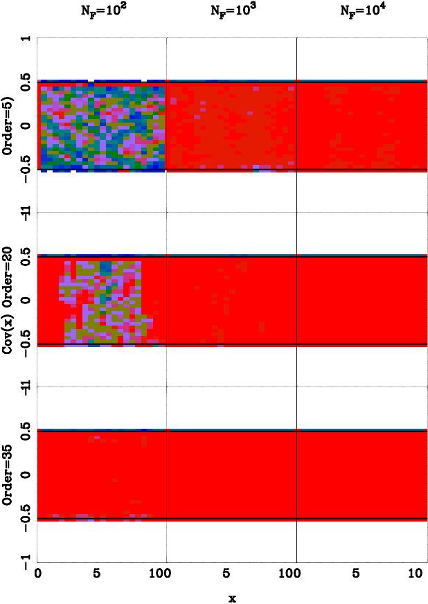
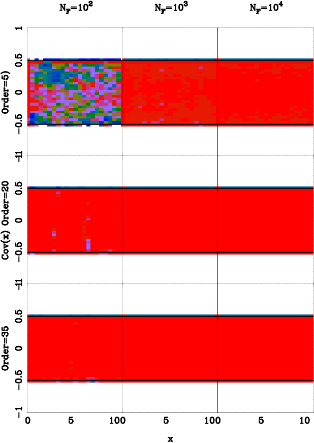
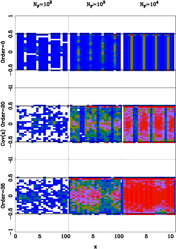
As expected when the functional order increases, and as the number of function evaluations increases, the number of pixels that experience all functional dependencies increases. We find that a maximum order of with realisations is sufficient for each point in the bounded area to experience every functional form for this simple example.
For the tophat basis set (binning) we find that the maximum order (number of bins) needs to be much larger than for either Chebyshev or Fourier basis sets. This can be understood since if the bin width (order) is larger than the resolution of the pixels then it is impossible for any given pixel to experience particular functional dependencies (such as [enter , exit ]). So even though tophat functions can be used for functional form filling there is some computational expense in this choice.
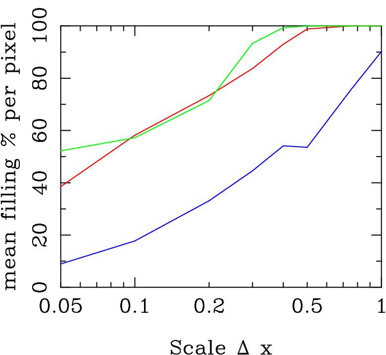
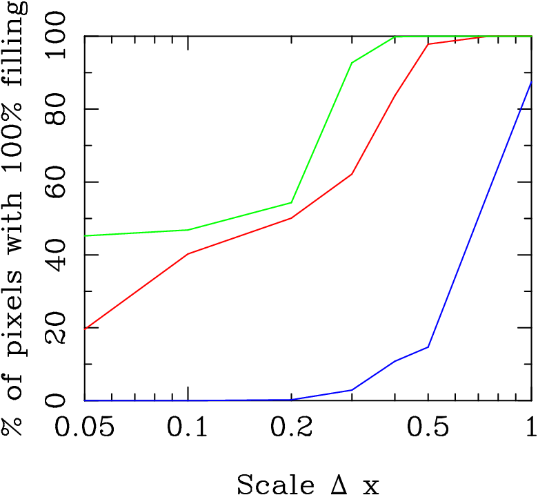
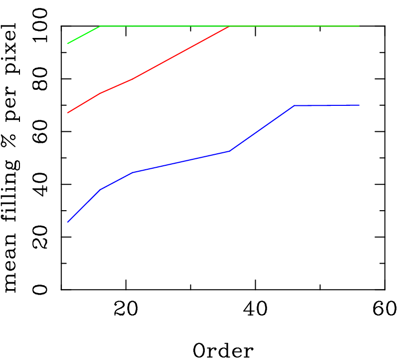
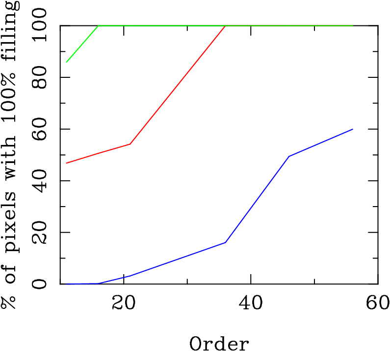

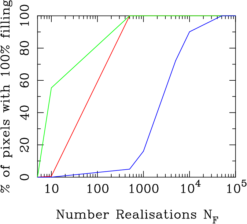
Fig. 18 shows some diagnostic plots representing the completeness of the functional space sampled. We show the percent of pixels that have 100% of the possible functional behaviours sampled, and the percentage of functional behaviours sampled by the average pixel. In the top panels we vary the scale that is investigated, and it can be seen that for the Chebyshev and Fourier basis sets of pixels have experienced every functional behaviour down to a scale of . The tophat basis set performs much worse with a mean filling of , and only of all pixels experiencing every possible behaviour. The general trend is that as the scale drops below the average oscillation length of the most highly varying functions the percentage of ‘good’ pixels (experiencing all functional behaviour) sharply declines. The tophat basis set fails at since, with this is approximately the ‘bin width’ of the functions. In a cosmological application one would ensure that the form filling was complete down to the scale upon which a particular parameter affects the signal.
In the middle panels of Fig. 18 we vary the maximum order of the basis set expansion whilst keeping both the scale and the number of random realisations fixed. It can again be seen that for a maximum order the Chebyshev and Fourier basis sets achieve 100% functional filling. Again the tophat basis set (binning) fails to achieve any complete functional filling, and only begins to fill in some pixels when the number of bins becomes more than the number of pixels.
The lower panel of Fig. 18 shows how the filling efficiency varies with the number of random realisations of the basis set. For the simple example given the Chebyshev and Fourier basis sets completely fill the bounded area, down to the scale of in realisations whereas the tophat basis set requires many orders of magnitude more realisations.
One could imagine futher metrics that could be used to gauge the completeness of the functional space that has been sampled, in this first exposition of the methodology we have shown a simple way to gauge this effect.
One concern is that this metric may favour the tophat basis since we are using a pixelated measure of scale. However we find that even with this advantage the tophat basis set achieves complete filling only at the expense of a prohibitive amount of computational time compared to the Chebyshev and Fourier basis sets, as the order and the number of realisations would need to be much larger to compensate for the pathological choice of basis functions.
We note that a step-function (e.g. function over the interval which is equal to for and for ) may be better approximated by a low order tophat function and may take a very high order Chebyshev or Fourier expansion. The feature highlighted here – a step function – has a feature (the step) which has a very small scale variation. In fact the scale of a step is actually zero. The issue of wether functional form filling is complete down to some scale is shown in Fig. 18, and as the maximum order is increased and more highly oscillatory functions are included the minimum complete scale will decrease. This example highlights that fact that the tophat basis set can probe these very small scales to some degree whilst missing larger scale features, this can be seen in Fig. 17.
For all the calculations in Section 4 we pessimistically use a maximum order of and use realisations for all basis sets.
Appendix C : Computational Time
One may be concerned at the amount of computational time that the functional form filling we are advocating may take. This is a valid convern since many realisations of the systematic data could be required and one must re-perform the cosmological parameter fitting for each and every possible function in order to evaluate the potential bias.
If, for a simple grid search in parameter space, the time taken to analyse a single point in parameter space is then for cosmological parameters the total time scales as where is the number of evaluations per parameter. Even for one parameter to correctly map out a likelihood surface. If one marginalises over extra systematic parameters then the total time must increase to . For the functional form filling case the total time taken for the calculation is simply the number of different function evaluations multiplied by the number of data realisations and the time to estimate the cosmological parameters is . The ratio in the computation time can now be written as .
Let us pessimistically assume that approximately function evaluations are needed and data realisations, and conservatively assume that extra systematic parameters are required to ensure a systematic effect is correctly determined. For we find . So on the contrary to such a technique being computationally expensive, treating systematics in such a fashion may in fact be much more efficient than marginalising over many nuisance parameters using a traditional grid search.
For some Monte Carlo parameter searches the computational time can be reduced to . In this case we find that . The computation time is now longer for functional form filling . This highlights the paramount importance of finding efficient form filling functions such as Chebyshev polynomials; we investigate the efficiency of Chebyshev, Fourier and tophat basis sets in Appendix B.
We take random realisations of the coefficient-space to uniformly sample the coefficients’ possible values. This is a first, brute-force attempt at the problem. Alternative approaches could explore a set grid of values in this space, or use a more sophisticated random search such as a Monte Carlo chain approach – we leave this for future work.
In this first investigation we have taken a simplistic approach and, as shown in Appendix B, we have found that a set of simple uniform random realisations is sufficient to explore the full space of functions.
Bayesian vs. Frequentist One may be concerned that what we are advocating is a frequenist solution to the systematic problem. On contrary what we suggest is explicitly Bayesian : the method can take into account any prior information on the systematic from either theory or data. The specific method used in this article to find the form filling functions is analogous to a brute force parameter in maximum likelihood rescontruction.
Appendix D : Extremal of the Bias
Here we will show that given a hard boundary or some data there exists a maximum absolute bias. Within the Fisher matrix formalism the bias caused by a function can be written (equation 12) as
| (87) |
where is the observed signal variance. We can rewrite this as
| (88) |
where , we compress this to
| (89) |
where .
We have the additional constraint that we are considering the set of systematic functions that give the same weight
| (90) |
with respect to some data vector . In this proof and throughout the article we assume that there is at least some systematic information at every data value in te signal. If there was no constraint at the position of some of the signal data values then the bias would be unbounded.
For the hard boundary there is a constraint that at all – this is actually for a constant (flat) hard boundary for a variable boundary the .
So to find the maximum bias we need to solve the following equation
| (91) |
where is a Langrange multiplier. Solving this for fixed and all we find that
| (92) |
To determine the value of the Lagrange multiplier we substitute this back into the constraint equation (90) to get a quadratic in
| (93) |
This has solutions of the form
| (94) |
where
| . | (95) |
So the function(s) with the maximum bias can be expressed as
| (96) |
Note that there exists two functions that represent the maximum and minimum bias, which are given by
| (97) |
So for a set of systematic functions that give the same weight with respect to some data there should exists a maximum and a minimum bias. Equation (90) can be understood by looking at Fig. 7. For the data boundary case there will be some large and small biases - actually every bias is ‘allowed’ but has some probability with repsect to the data. Equation (90) effectively takes a horizontal cut across on of the scatter plot panels in Fig. 7 at a given weight so that equation (97) gives the minimum and maximum biases for that weight.
If the mean of the data is zero and the variance of the data is then and
| (98) |
so that the mean bias is zero and the bias contours (contours are drawn for a constant weights, ) can be written as
| (99) |
For a hard boundary we have
| (100) |
which gives solutions for the maximum bias
| (101) |
this calculation can be compared to equations (98) and (99). This confirms that in the hard boundary case the absolute value of the bias has a maximum and that there exists two mirrored functions ( and ) which both yield this maximum absolute bias.
In the case when the systematic is constrained by some data points , we can easily construct a function that goes through all the systematic data points but has unbounded “bad effects” at some other point. However such a function, that has the same fit to the data but some other behaviour between the points is also assessed in terms of its impact on the cosmological parameter in question. Looking at Figure (7) such a function would have the same weight but would have a smaller bias than a “good function” that went through the same data points because the behaviour is not strongly degenerate with some “bad behaviour” but has a simple functional dependency.
The key conclusion of this Appendix is that out of the space of all functions that have the same weight with respect to the data there exists a maximum and a minimum bias that this space of functions can cause.
Appendix E: Data Weighting
We know that given some error bars on data, and a different realisation of the experiment, that the actual data points would be scattered differently but the statistical spread of the data would be the same. If a line fits exactly through some data points it is given a likelihood of exactly but we know that this probability is spurious since given another realisation of the experiment the data would be differently scattered and a new function would be assigned a probability of 1. This is a problem because should be unique. This problem occurs because in the original step the probability of the data has not been taken into account.
For the specific Gaussian case only we have used the marginalisation over the probability of the data can be done analytically. We stress here that in general the systematic mean will be non-zero and that only in this very simplified Gaussian case (and some other analytic examples) can this procedure can ve done anlytically.
Here we will outline how this ‘sample variance effect’ – that of taking into account the likelihood of the systematic data – can be incorporated into the weighting scheme given in equation (26).
We can write the probability of a function as the sum over the data vector multiplied by some prior probability of the data values
| (102) |
where are the function values are the variable positions at which the data has been taken.
We now want to marginalise over the probability of each data point to obtain
| (103) | |||||
Since we assume Gaussian data throughout the probability of the data can be written as a Gaussian centered about zero and can be replaced with a distribution such that
| (104) |
where is the error on the data point and and is the variance of data which we take to be . Note that each data point could have a different error bar - we have made the assumption that the data at each point is Gaussian distributed not that all data points are the same (the integral is over not over ). Evaluating the integral in equation (104) we have (now using log-likelihood for clarity)
| (105) |
So that in the case of Gaussian distributed data the probability of each function (and hence the probability of the bias incurred by that function) can be simply evaluated using equation (105). Note that a Gaussian with a mean of zero is unqiuely defined by its variance hence the data values themselves do not appear in the weighting formula given.
Appendix F : iCosmo module description
The ‘worst bias’ calculations presented in Section 5 were done using an extension to the open source interactive cosmology calculator iCosmo (Refregier et al., 2008b; http://www.icosmo.org). This additional module will be included in v and later.
The tomographic lensing module mk_bias_cheb takes and defined in equation (37) and uses the functional form filling technique (using the Chebyshev basis set) to calculate the maximum bias in each cosmological parameter. The lensing survey and central cosmology can be arbitrarily defined using the common set_fiducial routine described in Refregier et al. (2008b).