A universality result for the smallest eigenvalues of certain sample covariance matrices

Ohad N. Feldheim Sasha Sodin

Abstract

After proper rescaling and under some technical assumptions, the smallest eigenvalue of a sample covariance matrix with aspect ratio bounded away from $1$ converges to the Tracy–Widom distribution. This complements the results on the largest eigenvalue, due to Soshnikov and Péché.

Part I Introduction

¹¹footnotetext: [ohadfeld; sodinale]@post.tau.ac.il; address: School of Mathematical Sciences, Tel Aviv University, Ramat Aviv, Tel Aviv 69978, Israel²²footnotetext: Supported in part by the Adams Fellowship Program of the Israel Academy of Sciences and Humanities and by the ISF.

It has been long conjectured that some of the asymptotic statistical properties that are known for eigenvalues of large matrices with Gaussian entries should be valid, in particular, for more general random matrices with independent entries. This is part of a phenomenon called ‘universality’ in the physical literature; see for example Conjecture 1.2.1, Conjecture 1.2.2, and various remarks scattered in Mehta’s book [15].

In particular, the local statistics of the eigenvalues at the edge of the spectrum should be the same as in the Gaussian case (precise definitions are provided below.)

The first rigorous results of this kind are due to Soshnikov. In [21], he established a universality result at the edge for large Hermitian matrices with independent entries; we formulate his result as Theorem I.1.3 below. Universality at the edge for Hermitian random matrices with independent entries was further studied by Ruzmaikina [18] and Khorunzhiy and Vengerovsky [9].

In the subsequent work [22], Soshnikov extended his method to the largest eigenvalues of the sample covariance matrices $XX^{\ast}$ , under some restrictions on the dimensions of the matrices $X$ . These restrictions were later disposed of by Péché [16]; see Theorem I.1.2 below.

In the Hermitian case, the largest and the smallest eigenvalues are identically distributed; Soshnikov’s result encompasses both the largest and the smallest eigenvalue. The state of affairs is different for sample covariance matrices, the smallest eigenvalue of which is much smaller in absolute value than the largest one. Therefore Soshnikov’s approach does not seem to be applicable to the smallest eigenvalue of a sample covariance matrix; we discuss this further below.

In this paper, we suggest a different approach, and apply it to prove a universality result for the smallest eigenvalue of a sample covariance matrix; see Theorem I.1.1 below. We also apply it to give another proof of the results of Soshnikov and Péché, Theorems I.1.3 and I.1.2.

In the special case of Gaussian matrices, alternative approaches are available, and most of the results are known. The asymptotic distribution of the extreme eigenvalues of Gaussian Hermitian matrices has been first studied by Bronk [4] in the 1960-s, and more recently by Bowick and Brézin, Moore, Forrester, and finally by Tracy and Widom, who have established the conclusion of Theorem I.1.3 in the Gaussian case. Parallel results for Gaussian sample covariance matrices have been proved by Johansson, Johnstone, and Soshnikov, and Borodin and Forrester. We defer the precise references to Section I.3.

In fact, our argument (as well as those of Soshnikov and Péché) involves reduction to the Gaussian case. We discuss this in detail in Section I.3.

I.1 Formulation of results

The entries of the random matrices that we shall consider in this paper will be (complex-valued) random variables $r$ satisfying the following assumptions:

(A1): the distribution of $r$ is symmetric (that is, $r$ and $-r$ are identically distributed);
(A2): $\mathbb{E}|r|^{2k}\leq(C_{0}k)^{k}$ for some constant $C_{0}>0$ ( $r$ has subgaussian tails.)

Also, we shall assume that either

(A3₁): $\mathbb{E}r^{2}=\mathbb{E}r\bar{r}=1$ (or equivalently, $r$ is real almost surely and $\mathbb{E}r^{2}=1$ )

(A3₂): $\mathbb{E}r^{2}=0$ ; $\mathbb{E}r\bar{r}=1$ (that is, $\mathbb{E}(\Re r)^{2}=\mathbb{E}(\Im r)^{2}=1/2,\,\mathbb{E}(\Re r\,\Im r)=0$ .)

Our main result is

Theorem I.1.1.

Fix $\beta\in\{1,2\}$ . Let $\{X^{(N)}\}_{N}$ be a sequence of $M(N)\times N$ matrices, $M(N)\leq N$ , such that

1.

$\lim_{N\to+\infty}M(N)=+\infty$ ; $\limsup_{N\to+\infty}M(N)/N<1$ ;
2.

$\{X^{(N)}_{uv}\,|\,1\leq u\leq M(N),\,1\leq v\leq N\}$ are independent and satisfy (A1),(A2), and (A3_β).

Let $\lambda_{1}^{(N)}$ be the smallest eigenvalue of $B^{(N)}=X^{(N)}{X^{(N)}}^{\ast}$ . Then the random variable

\frac{\lambda_{1}^{(N)}-(M(N)^{1/2}-N^{1/2})^{2}}{(M(N)^{1/2}-N^{1/2})\left(M(N)^{-1/2}-N^{-1/2}\right)^{1/3}}

converges in distribution to the Tracy–Widom law $TW_{\beta}$ (cf. Section I.4) as $N\to\infty$ ¹¹ 1 $M(N)\leq N$ , so the denominator is negative. This is not a typo..

Our method also yields new proofs of two known results. The complementary result for the largest eigenvalue was proved by Soshnikov [22] (under additional restrictions on $M(N)$ ) and Péché [16] (in this generality):

Theorem I.1.2 (Soshnikov; Péché).

Fix $\beta\in\{1,2\}$ . Let $\{X^{(N)}\}_{N}$ be a sequence of $M(N)\times N$ matrices, $M(N)\leq N$ , such that

1.

$\lim_{N\to+\infty}M(N)=+\infty$ ;
2.

$\{X^{(N)}_{uv}\,|\,1\leq u\leq M(N),\,1\leq v\leq N\}$ are independent and satisfy (A1),(A2), and (A3_β).

Let $\lambda_{M(N)}^{(N)}$ be the largest eigenvalue of $B^{(N)}=X^{(N)}{X^{(N)}}^{\ast}$ . Then the random variable

\frac{\lambda_{M(N)}^{(N)}-(M(N)^{1/2}+N^{1/2})^{2}}{(M(N)^{1/2}+N^{1/2})\left(M(N)^{-1/2}+N^{-1/2}\right)^{1/3}}

converges in distribution to the Tracy–Widom law $TW_{\beta}$ .

The analogous theorem for Hermitian matrices was also proved by Soshnikov [21], and was the first universality result at the edge of the spectrum for matrices with independent entries. It was further studied by Ruzmaikina [18], and Khorunzhiy and Vengerovsky [9].

Theorem I.1.3 (Soshnikov).

Fix $\beta\in\{1,2\}$ . Let $\{A^{(N)}\}_{N}$ be a sequence of Hermitian $N\times N$ matrices such that $\{A^{(N)}_{uv}\,|\,1\leq u\leq v\leq N\}$ are independent and satisfy (A1),(A2), and, for $u<v$ , (A3_β). Let

\lambda_{1}^{(N)}\leq\cdots\leq\lambda_{N}^{(N)}

be the eigenvalues of $A^{(N)}$ . Then the random variables

-(N^{1/6}\lambda_{1}^{(N)}+2N^{2/3}),\quad N^{1/6}\lambda_{N}^{(N)}-2N^{2/3}

converge in distribution to the Tracy–Widom law $TW_{\beta}$ .

Most of this paper is devoted to the proofs of Theorems I.1.1-I.1.3. In the following section (I.2), we state slightly more general results in terms of point processes. Some of the definitions are postponed to Section I.4. There we also explain why the formulations of Section I.2 imply those of Section I.1. In Section I.5 we formulate two technical statements, and deduce the results of Section I.2. A guide to the subsequent sections, which are mostly devoted to the proof of the two technical statements, is provided at the end of Section I.5.

I.2 Formulation of results: extended version

Let us recall the definition of a point process and introduce a (slightly unusual) topology.

Definition I.2.1.

1.

A point process $\xi$ on $\mathbb{R}$ is a random integer-valued locally finite Borel measure on $\mathbb{R}$ .
2.

Let $\xi_{1},\xi_{2},\cdots,\xi_{N},\cdots;\xi$ be point processes on $\mathbb{R}$ . We shall write $\xi_{N}\overset{D}{\rightharpoonup}\xi$ if $\int fd\xi_{N}\overset{D}{\rightarrow}\int fd\xi$ (in distribution) for any bounded $f\in C(\mathbb{R})$ such that $\operatorname{supp}f\cap\mathbb{R}_{-}$ is compact.

Theorem I.2.2.

Under the assumptions of Theorem I.1.1, let

\lambda_{1}^{(N)}\leq\lambda_{2}^{(N)}\leq\cdots\leq\lambda_{M(N)}^{(N)}

be the eigenvalues of $B^{(N)}=X^{(N)}{X^{(N)}}^{\ast}$ , and let

y_{i}=\frac{\lambda_{i}^{(N)}-(M(N)^{1/2}-N^{1/2})^{2}}{(M(N)^{1/2}-N^{1/2})\left(M(N)^{-1/2}-N^{-1/2}\right)^{1/3}}~.

Then the point processes

\xi^{(N)}=\sum\delta_{y_{i}}

converge in distribution to the Airy point process $\mathfrak{Ai}_{\beta}$ :

\xi^{(N)}\overset{D}{\rightharpoonup}\mathfrak{Ai}_{\beta}~.

We shall recall the definition of $\mathfrak{Ai}_{\beta}$ in Section I.4.

Theorem I.2.3 (Soshnikov; Péché).

Under the assumptions of Theorem I.1.2, let

\lambda_{1}^{(N)}\leq\lambda_{2}^{(N)}\leq\cdots\leq\lambda_{M(N)}^{(N)}

be the eigenvalues of $B^{(N)}=X^{(N)}{X^{(N)}}^{\ast}$ , and let

y_{i}=\frac{\lambda_{M(N)-i+1}^{(N)}-(N^{1/2}+M(N)^{1/2})^{2}}{(M(N)^{1/2}+N^{1/2})\left(M(N)^{-1/2}+N^{-1/2}\right)^{1/3}}~.

Then the point processes

\eta^{(N)}=\sum\delta_{y_{i}}

converge in distribution to the Airy point process $\mathfrak{Ai}_{\beta}$ .

Theorem I.2.4 (Soshnikov).

Under the assumptions of Theorem I.1.3, let

\lambda_{1}^{(N)}\leq\lambda_{2}^{(N)}\leq\cdots\leq\lambda_{N}^{(N)}

be the eigenvalues of $A^{(N)}$ , and let

y_{i}^{\prime}=-(N^{1/6}\lambda_{i}^{(N)}+2N^{2/3}),\quad y_{i}=N^{1/6}\lambda_{N-i+1}^{(N)}-2N^{2/3}

Then the point processes

\xi^{(N)}=\sum\delta_{y_{i}^{\prime}}

and

\eta^{(N)}=\sum\delta_{y_{i}}

converge in distribution to the Airy point process $\mathfrak{Ai}_{\beta}$ .

I.3 Some Remarks

The most important example of random matrices satisfying the assumptions of Theorems I.1.1,I.1.2 is the Wishart Ensemble:

Example I.3.1.

1.

For $\beta=1$ , $X^{(N)}_{uv}\sim N(0,1)$ ;
2.

For $\beta=2$ , $X^{(N)}_{uv}\sim N(0,1/2)+iN(0,1/2)$ (meaning that the real and imaginary parts of $X^{(N)}_{uv}$ are independent Gaussian variables.)

We denote the random matrix $X^{(N)}$ by $X^{(N)}_{\text{inv}}$ (suppressing the dependence on $\beta$ ), and set $B^{(N)}_{\text{inv}}=X^{(N)}_{\text{inv}}{X^{(N)}_{\text{inv}}}^{\ast}$ .

Similarly, the most important example of random matrices satisfying the assumptions of Theorem I.1.3 is the Gaussian Orthogonal/Unitary Ensemble:

Example I.3.2.

1.

$\beta=1$ : in the Gaussian Orthogonal Ensemble (GOE),

$A^{(N)}_{uv}\sim\begin{cases}N(0,1)~,&u\neq v\\ N(0,2)~,&u=v~.\end{cases}$
2.

$\beta=2$ : in the Gaussian Unitary Ensemble (GUE),

$A^{(N)}_{uv}\sim\begin{cases}N(0,1/2)+iN(0,1/2)~,&u\neq v\\ N(0,1)~,&u=v~.\end{cases}$

We denote the matrix $A^{(N)}$ defined above by $A_{\text{inv}}^{(N)}$ .

The main feature of these examples is the invariance property: the distribution of $A_{\text{inv}}^{(N)}$ , $B^{(N)}_{\text{inv}}$ is invariant under conjugation by arbitrary orthogonal matrices (for $\beta=1$ ) or unitary matrices (for $\beta=2$ ). This feature facilitates the study of the eigenvalues of these matrices, and indeed, most of the results have been proved much earlier in this special case.

In particular, the conclusion of Theorem I.2.4 was proved for $A_{\text{inv}}^{(N)}$ in the early 90-s, by Bowick and Brézin, Forrester, Moore, and others, building on earlier work by Wigner, Dyson, and Mehta (see [15, 24] and references therein.)

The conclusion of Theorem I.2.3 was established for the invariant case $B^{(N)}_{\text{inv}}$ by Johansson [7] (for $\beta=2$ ) and Johnstone [8] (for $\beta=1$ ); see also Soshnikov [22]. The conclusion of Theorem I.2.2 was proved for $B^{(N)}_{\text{inv}}$ by Borodin and Forrester [3], under the weaker assumption $N-M(N)\to+\infty$ (instead of $\limsup M(N)/N<1$ ).

It has been long conjectured that, in the asymptotic limit $N\to\infty$ , some of the statistical properties that were proved for the eigenvalues of matrices with Gaussian entries should be valid, in particular, for more general random matrices with independent entries. See for example Conjecture 1.2.1, Conjecture 1.2.2, and various remarks scattered in Mehta’s book [15]. In particular, this should be true for local statistics of the eigenvalues at the edge of the spectrum.

The first rigorous results of this kind are due to Soshnikov. In [21], he established Theorem I.2.4. The main step in his proof is to show that the asymptotics of the mixed moments

\mathbb{E}\operatorname{tr}{A^{(N)}}^{m_{1}}\cdots\operatorname{tr}{A^{(N)}}^{m_{k}}~,

(I.3.1)

does not depend on the distribution of the entries of $A^{(N)}$ , when $\beta$ is fixed and $m_{1},\cdots,m_{k}=O(N^{2/3})$ . This reduces Theorem I.2.4 to the invariant case $A^{(N)}_{\text{inv}}$ .

In the subsequent work [22], Soshnikov applied a similar method to the largest eigenvalues of the sample covariance matrices $B^{(N)}$ , and proved Theorems I.1.2,I.2.3, under some additional restrictions on $M(N)$ . These restrictions were later disposed of by Péché [16].

This method does not seem to be directly applicable to the smallest eigenvalue of $B^{(N)}$ , since the asymptotics of (I.3.1) does not depend on the eigenvalues that are small in absolute value. In this paper, we make use of a modified technique, using traces of certain orthogonal polynomials of $A^{(N)}$ , $B^{(N)}$ . This technique is based on an idea going back to Bai and Yin [2], which was developed in several subsequent works; see [20] and references therein.

I.4 More definitions

For the convenience of the reader, we provide some definitions; this section is copied, up to change of notation, from the work of Soshnikov [21].

Definition I.4.1.

The measure $\rho_{k}=\rho_{k,\xi}=\mathbb{E}\xi^{\otimes k}$ on $\mathbb{R}^{k}$ is called the $k$ -point correlation measure of a point process $\xi$ .

Remark I.4.2.

Thus defined, the correlation measures have singular components on the diagonals $\{x_{1}=x_{2}\}$ , et cet. It is common to modify the definition to annihilate these singular components. However, the modified correlation measures $\tilde{\rho}_{k}$ are uniquely determined by $\rho_{k}$ , and vice versa; thus the difference is not very essential, and we find it more convenient to work with $\rho_{k}$ as above.

Remark I.4.3.

In general, a point process is not uniquely defined by its correlation measures. However, a sufficient condition due to Lenard [14] ensures uniqueness for the processes that we encounter in this paper.

For the sequel, let us introduce a topology on measures:

Definition I.4.4.

Let $\{\mu_{N}\}$ be a sequence of measures on $\mathbb{R}^{k}$ . We shall write $\mu_{N}\rightharpoonup\mu$ if $\int fd\mu_{n}\to\int fd\mu$ for any bounded continuous function $f$ on $\mathbb{R}^{k}$ such that $\operatorname{supp}f\cap\mathbb{R}_{-}^{k}$ is compact.

Definition I.4.5.

The Airy function $\operatorname{Ai}$ is (uniquely) defined by

\operatorname{Ai}^{\prime\prime}(x)=x\operatorname{Ai}(x)~,\qquad\operatorname{Ai}(x)\sim\frac{1}{2\sqrt{\pi}x^{1/4}}\exp\left(-\frac{2}{3}x^{3/2}\right)~,\quad x\to+\infty~.

Definition I.4.6.

The Airy point process $\mathfrak{Ai}_{2}$ is the (unique) point process such that, for every $k$ and any compact set

T\subset\left\{(x_{1},\cdots,x_{k})\,\big|x_{1}<\cdots<x_{k}\right\}~,

the restriction $\rho_{k}|_{T}$ is absolutely continuous with respect to the Lebesgue measure, and

\frac{d\rho_{k}|_{T}(x_{1},\cdots,x_{k})}{dx_{1}\cdots dx_{k}}=\det\Big(K(x_{i},x_{j})\Big)_{1\leq i,j\leq k}~,

where

K(x,x^{\prime})=\frac{\operatorname{Ai}(x)\operatorname{Ai}^{\prime}(x^{\prime})-\operatorname{Ai}^{\prime}(x)\operatorname{Ai}(x^{\prime})}{x-x^{\prime}}~.

2.

The Tracy–Widom law $TW_{2}$ is defined by its cumulative distribution function

$F_{2}(x)=\exp\left\{-\int_{x}^{+\infty}(s-x)q^{2}(s)ds~,\right\}$

where $q(\cdot)$ is the solution to the II ${}^{\text{nd}}$ Painlevé equation:

$q^{\prime\prime}(s)=sq(s)+2q(s)^{3}~,$

such that

$q(s)\sim\operatorname{Ai}(s)~,\quad s\to+\infty$

(the so-called Hastings–McLeod solution.)

For $\beta=1$ , the density of $\rho_{k}$ can be expressed as the square root of the determinant of a $2k\times 2k$ block matrix, which is composed of $2\times 2$ blocks. Denote

	$\displaystyle DK(x,x^{\prime})$	$\displaystyle=$	$\displaystyle-\frac{\partial}{\partial x^{\prime}}K(x,x^{\prime})~,$
	$\displaystyle JK(x,x^{\prime})$	$\displaystyle=$	$\displaystyle-\int_{x}^{+\infty}K(x^{\prime\prime},x^{\prime})dx^{\prime\prime}-\frac{1}{2}\operatorname{sign}(x-x^{\prime})~;$

then let

K_{1}(x,x^{\prime})=\left(\begin{array}[]{ccc}K(x,x^{\prime})&DK(x,x^{\prime})\\ JK(x,x^{\prime})&K(x,x^{\prime})\end{array}\right)~.

Definition I.4.7.

1.

The Airy point process $\mathfrak{Ai}_{1}$ is the (unique) point process such that, for every $k$ and any compact set

$T\subset\left\{(x_{1},\cdots,x_{k})\,\big|x_{1}<\cdots<x_{k}\right\}~,$

the restriction $\rho_{k}|_{T}$ is absolutely continuous with respect to the Lebesgue measure, and

$\frac{d\rho_{k}|_{T}(x_{1},\cdots,x_{k})}{dx_{1}\cdots dx_{k}}=\sqrt{\det\Big(K_{1}(x_{i},x_{j})\Big)_{1\leq i,j\leq k}}~.$
2.

The Tracy–Widom law $TW_{1}$ is defined by its cumulative distribution function

$F_{1}(x)=\exp\left\{-\int_{x}^{+\infty}\left[q(s)+(s-x)q^{2}(s)\right]ds\right\}~.$

Theorem (Tracy–Widom [24, 25]).

For $\beta\in\{1,2\}$ , the distribution of the rightmost atom of $\mathfrak{Ai}_{\beta}$ is exactly $TW_{\beta}$ .

The functional that sends a locally finite configuration of points (= locally finite integer-valued Borel measure) to its rightmost point (= atom) is continuous with respect to the convergence $\rightharpoonup$ , and therefore Theorem I.2.2 implies Theorem I.1.1, Theorem I.2.3 implies Theorem I.1.2, Theorem I.2.4 implies Theorem I.1.3.

I.5 The main technical statements

Definition I.5.1.

The Chebyshev polynomials of the second kind are defined as follows:

U_{n}(\cos\theta)=\frac{\sin((n+1)\theta)}{\sin\theta}~.

(I.5.1)

The following elementary proposition may clarify the connection between $U_{n}$ and the spectra of the matrices considered in this paper. We shall not use it, and therefore omit the proof (see e.g. [20, §5.1].)

Proposition I.5.2.

1.

The polynomials $U_{n}$ are the orthogonal polynomials with respect to Wigner’s semicircle measure $\sigma_{\text{W}}$ :

$\frac{d\sigma_{\text{W}}(x)}{dx}=\frac{2}{\pi}(1-x^{2})_{+}^{1/2}~.$

That is,

$\int U_{n}(x)U_{n^{\prime}}(x)d\sigma_{\text{W}}(x)=\delta_{nn^{\prime}}~.$
2.

For $0\leq s\leq 1$ , the polynomials $V_{n,s}=U_{n}+\sqrt{s}U_{n-1}$ are orthogonal with respect to the Marchenko–Pastur measure $\sigma_{\text{MP}}^{(s)}$ :

$\frac{d\sigma_{\text{MP}}^{(s)}(x)}{dx}=\frac{2}{\pi}\frac{(1-x^{2})_{+}^{1/2}}{(1+s)+2\sqrt{s}x}~.$

In the next parts of this paper we shall prove the following two statements:

Theorem I.5.3.

Fix $\beta\in\{1,2\}$ , and let $\{A^{(N)}\}$ be a sequence of random matrices satisfying the assumptions of Theorem I.1.3. Fix $k\geq 1$ , and let $\{(n_{1}^{(N)},\cdots,n_{k}^{(N)})\}_{N}$ be a sequence of $k$ -tuples.

1.

If $\sum n_{i}^{(N)}\equiv 1\mod 2$ ,

$\mathbb{E}\prod_{i=1}^{k}\operatorname{tr}U_{n_{i}^{(N)}}(A^{(N)}/(2\sqrt{N-2}))=0~.$

Suppose $\sum n_{i}^{(N)}=2n^{(N)}$ . There exists a constant $C$ (depending only on $C_{0}$ in (A2)), such that

\mathbb{E}\prod_{i=1}^{k}\operatorname{tr}U_{n_{i}^{(N)}}(A^{(N)}/(2\sqrt{N-2}))\leq(Cn^{(N)})^{k}\,\exp\left\{C{n^{(N)}}^{3/2}/{N^{1/2}}\right\}~.

If moreover $n^{(N)}=O(N^{1/3})$ ,

\mathbb{E}\prod_{i=1}^{k}\operatorname{tr}U_{n_{i}^{(N)}}(A^{(N)}/(2\sqrt{N-2}))\\ =\mathbb{E}\prod_{i=1}^{k}\operatorname{tr}U_{n_{i}^{(N)}}(A_{\text{inv}}^{(N)}/(2\sqrt{N-2}))+o((n^{(N)})^{k})

as $N\to+\infty$ , where $A_{\text{inv}}^{(N)}$ is as in Example I.3.2, and the implicit constant in $o(\cdots)$ may depend on $k$ , $C_{0}$ , and $n/N^{1/3}$ .

There are several ways to deduce Theorem I.2.4 from Theorem I.5.3. For example, one may use Levitan’s uniqueness theorem [14] for the transform

\mu\mapsto\mathfrak{T}(\mu),\quad\mathfrak{T}(\mu)(\alpha)=\int_{-\infty}^{+\infty}\frac{\sin(\alpha\sqrt{x})}{\alpha\sqrt{x}}d\mu(x)~,

which appears naturally from the asymptotics of $U_{n}$ near $\pm 1$ . However, the justification of convergence makes this approach quite cumbersome.

We shall follow Soshnikov’s original argument [21] and go back to moments and to the Laplace transform

\mu\mapsto\mathfrak{L}(\mu),\quad\mathfrak{L}(\mu)(\alpha)=\int_{-\infty}^{+\infty}\exp(\alpha x)d\mu(x)~.

Proof of Theorem I.2.4.

We shall use the following simple identities (see e.g. Snyder [19]):

	$\displaystyle x^{2m}$	$\displaystyle=$	$\displaystyle\frac{1}{(2m+1)2^{2m}}\sum_{n=0}^{m}(2n+1)\binom{2m+1}{m-n}U_{2n}(x)~;$		(I.5.2)
	$\displaystyle x^{2m-1}$	$\displaystyle=$	$\displaystyle\frac{1}{(2m)2^{2m-1}}\sum_{n=0}^{m}2n\binom{2m}{m-n}U_{2n-1}(x)~.$		(I.5.3)

Let us show that

1.

$\mathbb{E}\operatorname{tr}(A^{(N)}/(2\sqrt{N}))^{m}\leq\frac{C_{1}N}{m^{3/2}}\exp(C_{2}m^{3}/N^{2})$ , where $C_{1},C_{2}$ may depend on $C_{0}$ ;
2.

$\mathbb{E}\operatorname{tr}(A^{(N)}/(2\sqrt{N}))^{m}=\mathbb{E}\operatorname{tr}(A^{(N)}_{\text{inv}}/(2\sqrt{N}))^{m}+o(1)$ for $m=O(N^{2/3})$ , where the implicit constant in $o(1)$ may depend on $C_{0}$ and on $m/N^{2/3}$ .

(This is more or less the content of Theorem 2 in [21].) Substitute

x=A^{(N)}/(2\sqrt{N-2})

in (I.5.2) and take the expectation of the trace:

\mathbb{E}\operatorname{tr}\left[\frac{A^{(N)}}{2\sqrt{N-2}}\right]^{m}\\ =\frac{1}{(2m+1)2^{2m}}\sum_{n=0}^{m}(2n+1)\,\binom{2m+1}{m-n}\,\mathbb{E}\operatorname{tr}U_{2n}\left[\frac{A^{(N)}}{2\sqrt{N-2}}\right]~.

(I.5.4)

The $0$ -th term in (I.5.4) is equal to

\mathrm{TERM}_{0}=\binom{2m+1}{m}\,N\leq\frac{C\,2^{2m}\,N}{\sqrt{m}}~.

By the second item of Theorem I.5.3,

\begin{split}\mathrm{TERM}_{n}&\leq(2n+1)\binom{2m+1}{m-n}\,Cn\,\exp(Cn^{3/2}/N^{1/2})\\ &\leq 2^{2m}\,\frac{C^{\prime}n^{2}}{\sqrt{m}}\,\exp(-cn^{2}/m+Cn^{3/2}/N^{1/2})~.\end{split}

(I.5.5)

Thus

\mathbb{E}\operatorname{tr}\left[\frac{A^{(N)}}{2\sqrt{N-2}}\right]^{m}\\ \leq\frac{C2^{2m}}{\sqrt{m}}\frac{1}{m2^{2m}}\left\{N+\sum_{n=1}^{m}n^{2}\exp(-cn^{2}/m+Cn^{3/2}/N^{1/2})\right\}\\ \leq\frac{CN}{m\sqrt{m}}\exp(Cm^{3}/N^{2})~.

(I.5.6)

This proves 1.

The inequality (I.5.5) also ensures that the contribution of

n>C^{\prime}m^{2}/N+N^{1/3}

(with, say, $C^{\prime}=10$ ) is negligible. Hence one can restrict the sum to

n\leq C^{\prime}m^{2}/N+N^{1/3}~,

and apply the third item. This proves 2. for even values of $m$ ; for odd values of $m$ , both sides are zero.

Proceeding with Soshnikov’s argument, we deduce that the sequences $\{\xi^{(N)}\}$ , $\{\eta^{(N)}\}$ are precompact, and that

(4N)^{-m_{N}/2}\,\mathbb{E}\operatorname{tr}(A^{(N)})^{m_{N}}\to\int\exp(\alpha y)((-1)^{p}d\rho_{1,\xi}(y)+d\rho_{1,\eta}(y))

for any limit points $\xi$ , $\eta$ , as long as $m_{N}/N^{2/3}\to\alpha$ and $m_{N}$ is of constant parity $p$ . Therefore the Laplace transforms $\mathfrak{L}(\rho_{1,\xi}),\mathfrak{L}(\rho_{1,\eta})$ do not depend on the distribution of the entries of the matrix $A^{(N)}$ . In exactly the same way we show that $\mathfrak{L}(\rho_{k,\xi}),\mathfrak{L}(\rho_{k,\eta})$ are defined uniquely for any $k\geq 1$ , and hence are the same as for $A^{(N)}_{\text{inv}}$ . Therefore (again, see [21]), we deduce that

\xi^{(N)},\eta^{(N)}\overset{D}{\rightharpoonup}\mathfrak{Ai}_{\beta}~.

∎

Theorem I.5.4.

Fix $\beta\in\{1,2\}$ , and let $\{B^{(N)}\}$ be a sequence of random matrices satisfying the assumptions of Theorem I.1.2. Fix $k\geq 1$ , and let $\{(n_{1}^{(N)},\cdots,n_{k}^{(N)})\}_{N}$ be a sequence of $k$ -tuples.

Suppose $\sum n_{i}^{(N)}=n^{(N)}$ . There exists a constant $C$ (depending only on $C_{0}$ in (A2)), such that

\mathbb{E}\prod_{i=1}^{k}\operatorname{tr}V_{n_{i}^{(N)},M(N)/N}\left(\frac{B^{(N)}-(M(N)+N-2)}{2\sqrt{(M(N)-1)(N-1)}}\right)\\ \leq(Cn^{(N)})^{k}\,\exp\left\{C{n^{(N)}}^{3/2}/{M(N)^{1/2}}\right\}~.

If moreover $n^{(N)}=O(M(N)^{1/3})$ ,

\mathbb{E}\prod_{i=1}^{k}\operatorname{tr}V_{n_{i}^{(N)},M(N)/N}\left(\frac{B^{(N)}-(M(N)+N-2)}{2\sqrt{(M(N)-1)(N-1)}}\right)\\ =\mathbb{E}\prod_{i=1}^{k}\operatorname{tr}V_{n_{i}^{(N)},M(N)/N}\left(\frac{B_{\text{inv}}^{(N)}-(M(N)+N-2)}{2\sqrt{(M(N)-1)(N-1)}}\right)+o((n^{(N)})^{k})

as $N\to+\infty$ , where $B_{\text{inv}}^{(N)}$ is as in Example I.3.1, and the implicit constant in $o(\cdots)$ may depend on $k$ , $C_{0}$ , and $n/M(N)^{1/3}$ .

Similarly to the above, Theorem I.5.4 implies Theorems I.2.2,I.2.3.

Sketch of proof of Theorems I.2.2,I.2.3.

As in the proof of Theorem I.2.4, we consider moments. Expressing

\mathbb{E}\operatorname{tr}\left[\frac{B^{(N)}-(M(N)+N-2)}{2\sqrt{(M(N)-1)(N-1)}}\right]^{2m}\\ +\mathbb{E}\operatorname{tr}\left[\frac{B^{(N)}-(M(N)+N-2)}{2\sqrt{(M(N)-1)(N-1)}}\right]^{2m-1}

(I.5.7)

in terms of

\mathbb{E}\operatorname{tr}V_{n,M(N)/N}\left[\frac{B^{(N)}-(M(N)+N-2)}{2\sqrt{(M(N)-1)(N-1)}}\right]~,

one may check that the asymptotics of (I.5.7) is the same as for $B^{(N)}=B^{(N)}_{\text{inv}}$ . If $M(N)/N<1-\eta<1$ , the same is true for

\mathbb{E}\operatorname{tr}\left[\frac{B^{(N)}-(M(N)+N-2)}{2\sqrt{(M(N)-1)(N-1)}}\right]^{2m}\\ -\mathbb{E}\operatorname{tr}\left[\frac{B^{(N)}-(M(N)+N-2)}{2\sqrt{(M(N)-1)(N-1)}}\right]^{2m-1}

(I.5.8)

(with the implicit constants depending on $\eta$ .) From this point, proceed as in the proof of Theorem I.2.4. ∎

Remark I.5.5.

Taking Remarks II.3.5,IV.1.6 into account, one can actually avoid the use of any results for Wishart matrices, and compare the correlation measures to those in Theorem I.2.4.

Plan of the proceeding sections. Parts II,III are devoted to the proof of Theorem I.5.3. In Part II we focus on the special case of matrices the entries of which are uniformly distributed on the $(\beta-1)$ -dimensional sphere (except for the diagonal entries, which are zero, see (II.0.1) below.) We discuss the asymptotics of the expectations in Theorem I.5.3 in detail, first for $k=1$ , and obtain a certain “genus expansion”, Proposition II.2.5. In Section II.3 we extend these results to arbitrary $k\geq 1$ . This part is based on the connection to non-backtracking paths on the complete graph, which is very explicit and simple in the special case (II.0.1) (see Claim II.1.2 below).

In Part III we show that the results of Part II can be extended to matrices with arbitrary distribution of entries (that satisfy the conditions of Theorem I.1.3.) The three main technical difficulties that appear are:

1.

to express $\operatorname{tr}U_{n}(A/(2\sqrt{N-2}))$ as a sum over paths;
2.

to show that multiple edges do not contribute to the part of the asymptotics that comes from non-backtracking paths.
3.

to show that paths with backtracking do not contribute to the asymptotics of the expressions in Theorem I.5.3.

In Part IV we prove Theorem I.5.4. The asymptotics of the expressions in Theorem I.5.4 is closely connected to non-backtracking paths on the complete bipartite graph. Therefore the proofs mostly mimic the proofs in Parts II,III, and we mainly indicate the necessary modifications.

Part V is devoted to extensions and some remarks. We discuss additional results that can be proved using the methods of this paper, and indicate the modifications that should be made in the proofs. In particular, we discuss quaternionic random matrices (which correspond to $\beta=4$ ), and matrices with unequal real and imaginary part. In Section V.2 we discuss some deviation inequalities for the extreme eigenvalues.

Notation: The large parameter in this paper is $N\to\infty$ . For quantities $\phi,\psi$ depending on $N$ , we write $\phi\ll\psi$ for $\phi=o(\psi)$ , and $\phi\sim\psi$ for $\phi/\psi=1+o(1)$ ; $\phi=\Theta(\psi)$ if $\phi=O(\psi)$ and $\psi=O(\phi)$ . The letters $C,C^{\prime},C_{1},\cdots$ will stand for positive constants the value of which may vary from line to line. Some of these may depend on $C_{0}$ in (A2) or on other parameters; we mention it explicitly when this is the case.

Part II Matrices with uniform entries

In this part, we focus on the special cases

\begin{split}\beta=1,&\quad A_{uv}=\begin{cases}\pm 1\quad\text{with prob.\ $1/2$},&u\neq v~,\\ 0,&u=v~;\end{cases}\\ \beta=2,&\quad A_{uv}\sim\begin{cases}\textrm{unif}(S^{1}),&u\neq v~,\\ 0,&u=v~.\end{cases}\\ \end{split}

(II.0.1)

From this point, we suppress the dependence on $N$ in the notation.

II.1 Reduction to diagrams

Consider the following sequence of polynomials $P_{n}=P_{n,N}$ :

\begin{split}P_{0}(x)&=1,P_{1}(x)=x,P_{2}(x)=x^{2}-(N-1),\\ P_{n}(x)&=xP_{n-1}(x)-(N-2)P_{n-2}(x)\quad\text{for $n\geq 3$.}\end{split}

(II.1.1)

Lemma II.1.1.

The following identity holds:

\begin{split}&P_{n}(x)=(N-2)^{n/2}\\ &\qquad\times\left\{U_{n}\left(\frac{x}{2\sqrt{N-2}}\right)-\frac{1}{N-2}U_{n-2}\left(\frac{x}{2\sqrt{N-2}}\right)\right\}~,\end{split}

(II.1.2)

where formally $U_{-2}\equiv U_{-1}\equiv 0$ .

Proof.

For $n=0,1,2$ the identity (II.1.2) follows directly from (II.1.1), (I.5.1). Next, (I.5.1) implies (cf. [19]) that

U_{n}(y)=2yU_{n-1}(y)-U_{n-2}(y)~,\quad n=2,3,\cdots~.

(II.1.3)

Taking $y=x/(2\sqrt{N-2})$ , we see that the right-hand side of (II.1.2) satisfies the same recurrent relation as the left-hand side. ∎

Claim II.1.2.

For any Hermitian $N\times N$ matrix $A$ with zeros on the diagonal and other entries on the unit circle,

P_{n}(A)_{u_{0}u_{n}}=\sum_{p_{n}}A_{u_{0}u_{1}}A_{u_{1}u_{2}}\cdots A_{u_{n-1}u_{n}}~,

(II.1.4)

where the sum is over all paths $p_{n}=u_{0}u_{1}\cdots u_{n}$ such that

(a): $u_{j}\neq u_{j-1}$ for $j=1,\cdots,n$ ;
(b): $u_{j}\neq u_{j-2}$ for $j=2,\cdots,n$ (the non-backtracking condition).

Proof.

For $n=0,1$ the identity (II.1.4) is trivial. For $n\geq 2$ observe that

P_{n}(A)=P_{n-1}(A)A-(N-2)P_{n-2}(A)

(II.1.5)

according to (II.1.3), and on the other hand

A_{uv}A_{vu}=\begin{cases}1,&u\neq v\\ 0,&u=v\end{cases}

and hence the right-hand side of (II.1.4) also satisfies (II.1.5). ∎

By Claim II.1.2, the expectation $\mathbb{E}\operatorname{tr}P_{n}(A)$ is equal to the number of paths $p_{n}=u_{0}u_{1}\cdots u_{n}$ that satisfy the conditions (a),(b) (above) and (c),(d ${}_{\beta}^{1}$ ) (below):

(c)

$u_{n}=u_{0}$ ;

(d ${}_{1}^{1}$ )

for any $u\neq v$ ,

\#\left\{j\,|\,u_{j}=u,\,u_{j+1}=v\right\}\equiv\#\left\{j\,|\,u_{j}=v,\,u_{j+1}=u\right\}\mod 2~;

(d ${}_{2}^{1}$ )

for any $u\neq v$ ,

\#\left\{j\,|\,u_{j}=u,\,u_{j+1}=v\right\}=\#\left\{j\,|\,u_{j}=v,\,u_{j+1}=u\right\}~.

In particular, $\mathbb{E}\operatorname{tr}P_{2n+1}(A)=0$ , therefore we shall only study

\Sigma_{\beta}^{1}=\Sigma_{\beta}^{1}(2n)=\mathbb{E}\operatorname{tr}P_{2n}(A)~.

(II.1.6)

Let $p_{2n}=u_{0}u_{1}\cdots u_{2n}$ be a path satisfying (a), (b), (c), (d ${}_{\beta}^{1}$ ). Consider a directed multigraph $G=(V,E_{\text{dir}})$ , where $V\subset\{1,\cdots,N\}$ is the set of all vertices $u_{j}$ , and $E_{\text{dir}}$ is the set of edges $(u_{j-1},u_{j})$ (with multiplicities). A matching of $p_{2n}$ is a matching (= involution without fixed points) of $\{0,1,\cdots,2n-1\}$ , so that

•

for $\beta=1$ , every edge $(u,v)$ is matched either to a coincident edge $(u,v)$ or to $(v,u)$ ;
•

for $\beta=2$ , an edge $(u,v)$ is matched to $(v,u)$ .

A path together with a matching will be called a matched path.

Denote by ${\Sigma^{1m}_{\beta}}(2n)$ the number of matched paths (satisfying (a), (b), (c), (d ${}_{\beta}^{1}$ )), and denote by ${\Sigma_{\beta}}(2n)$ the number of paths satisfying (a), (b), (c) and the stronger condition (d_β):

(d₁)

for any $u\neq v$ ,

\#\left\{j\,|\,u_{j}=u,\,u_{j+1}=v\right\}+\#\left\{j\,|\,u_{j}=v,\,u_{j+1}=u\right\}\in\{0,2\}~.

(d₂)

for any $u\neq v$ ,

\#\left\{j\,|\,u_{j}=u,\,u_{j+1}=v\right\}=\#\left\{j\,|\,u_{j}=v,\,u_{j+1}=u\right\}\in\{0,1\}~.

Obviously,

\Sigma_{\beta}(2n)\leq\Sigma_{\beta}^{1}(2n)\leq\Sigma_{\beta}^{1m}(2n)~.

(II.1.7)

Our next goal is to study the asymptotics of $\Sigma^{1m}_{\beta}(2n)$ . In particular, we shall prove that

\Sigma_{\beta}^{1m}(2n)\leq\Sigma_{\beta}(2n)(1+o(1))

as long as $n=o(N^{1/2})$ .

Let us introduce some more graph-theoretical notation.

Definition II.1.3.

Let $\beta\in\{1,2\}$ .

•

A diagram of type $\beta$ is an (undirected) multigraph $\bar{G}=(\bar{V},\bar{E})$ , together with a circuit $\bar{p}=\bar{u}_{0}\bar{u}_{1}\cdots\bar{u}_{0}$ on $\bar{G}$ , such that

–

$\bar{p}$ is non-backtracking (meaning that no edge is followed by its reverse, unless the edge is $\bar{u}\bar{u}$ and $\beta=1$ );

–

For every $(\bar{u},\bar{v})\in\bar{E}$ ,

\begin{split}\#\left\{j\,|\,\bar{u}_{j}=\bar{u},\,\bar{u}_{j+1}=\bar{v}\right\}+\#\left\{j\,|\,\bar{u}_{j}=\bar{v},\,\bar{u}_{j+1}=\bar{u}\right\}=2\quad(\beta=1)~,\\ \#\left\{j\,|\,\bar{u}_{j}=\bar{u},\,\bar{u}_{j+1}=\bar{v}\right\}=\#\left\{j\,|\,\bar{u}_{j}=\bar{v},\,\bar{u}_{j+1}=\bar{u}\right\}=1\quad(\beta=2)~;\end{split}

–

the degree of $\bar{u}_{0}$ in $\bar{G}$ is 1; the degrees of all the other vertices are equal to 3.

•

A weighted diagram is a diagram $\bar{G}$ together with a weight function $\bar{w}:\bar{E}\to\{-1,0,1,2,\cdots\}$ .

Let us construct a mapping from the collection of matched paths satisfying (a), (b), (c), (d ${}_{\beta}^{1}$ ) into the collection of weighted diagrams (of type $\beta$ .)

(i) Start with the multigraph $G=G(p_{2n})=(V,E_{\text{dir}})$ corresponding to the path $p_{2n}$ :

V=\{u\,\mid\,\exists j,\,u_{j}=u\}~,\,\,E_{\text{dir}}=\{(u_{j},u_{j+1})\}~,

and unite each pair of matched edges into a single undirected edge.

(ii) If the degree of $u_{0}$ is greater than 1, add a vertex $r$ connected to $u_{0}$ , and replace $p_{2n}$ with $ru_{0}u_{1}\cdots u_{0}r$ . Otherwise set $r=u_{0}$ .

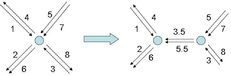
(iii) For every vertex $u\neq r$ of degree $d>3$ , replace $u$ with $\leq d-2$ vertices of degree $\leq 3$ using the inductive procedure illustrated in Figure 1.

(iv) Erase all the vertices of degree 2.

(v) Set

\bar{w}(\bar{e})=\begin{cases}\text{the number of erased vertices on $\bar{e}$}\\ -1,\quad\text{if $\bar{e}$ was created at {\bf(ii) - (iii)}}~.\end{cases}

Refer to caption — Figure 1: Splitting a vertex of high degree ( $\beta=1$ )

The above construction yields

Claim II.1.4.

There are at most $N^{\#\bar{V}+\sum_{\bar{e}}\bar{w}(\bar{e})}$ matched paths corresponding to a weighted diagram $(\bar{G},\bar{p},\bar{w})$ . If $\bar{w}(\bar{e})\geq 1$ for every $\bar{e}\in\bar{E}$ , there are exactly

N\big(N-1\big)\cdots\big(N-(\#\bar{V}+\sum_{\bar{e}}\bar{w}(\bar{e}))+1\big)

(II.1.8)

such paths. In particular, if $\bar{w}(\bar{e})\geq 1$ for every $\bar{e}\in\bar{E}$ , and if

\#\bar{V}+\sum_{\bar{e}}\bar{w}(\bar{e})=o(N^{1/2})~,

the number of matched paths and the number of paths (without a matching) are both

N^{\#\bar{V}+\sum_{\bar{e}}\bar{w}(\bar{e})}\,(1-o(1))~.

II.2 Counting diagrams

Let us present an automaton which constructs all possible diagrams. Consider first the case $\beta=2$ .

States: $(t;\ell_{1},\cdots,\ell_{k})$ , where $t,k\geq 0$ and $\ell_{j}>0$ ; initial state: $t=k=0$ . We can visualise the state of the automaton as a “thread” made of $t$ pieces, and $k$ “loops” (the $j$ -th loop is made of $\ell_{j}$ pieces).

There are 2 transitions for $\beta=2$ :

1.

(“creation” of a new loop, see Figure 2):

t\longleftarrow t^{\prime}\leq t+1~;\quad\ell_{1},\cdots,\ell_{k}\longleftarrow\ell_{1},\cdots,\ell_{k},\ell_{k+1}~,

where $\ell_{k+1}\leq t-t^{\prime}+2$ .

-1,0) (3, .5).50360 (3.7, 1.7).50360 (2.3, 1.7).5180185 (10, .5).50360 (10.7, 1.7).50360 (9.3, 1.7).5180180

Figure 2: Transition 1.

2.

(“annihilation” of the $j$ -th loop, see Figure 3):

t\longleftarrow t^{\prime}\leq t+\ell_{j}+2~;\quad\ell_{1},\cdots,\ell_{k}\longleftarrow\ell_{1},\cdots,\ell_{j-1},\ell_{j+1},\cdots,\ell_{k}~.

-1,0) (3, .5).50360 (3.7, 1.7).50360 (2.3, 1.7).50360 , 1.7).6160-20 (10, .5).60360 (10.7, 1.7).50360 (9.3, 1.7).6160-20

Figure 3: Transition 2. for

\beta=2

We impose the restriction $t>0$ all along the way, and demand that after some (even) number of steps $s=2g$ the automaton return to the original state and stop.

Claim II.2.1.

Every diagram (corresponding to $\beta=2$ ) is generated by the automaton. If the automaton stops after $s=2g$ steps, the diagram has $\#\bar{E}=6g-1=3s-1$ edges and $\#\bar{V}=4g=2s$ vertices.

Proof.

It suffices to observe that the first (creation) step creates 3 edges and 3 vertices, the last (annihilation) step creates 2 edges and one vertex, and every other step creates 3 edges and 2 vertices. ∎

Denote by $D_{2}(s)$ the number of diagrams corresponding to $s$ steps (of course, $D_{2}(s)=0$ for odd values of $s$ .)

For $\beta=1$ , the transitions are slightly different. First, every time a loop is annihilated (transition 2.), the automaton has to choose a direction in which the loop is passed. That is, there are two possibilities: the one in Figure 3, and the one in Figure 4.

-1,0) (3, .5).50360 (3.7, 1.7).50360 (2.3, 1.7).50360 (2.3, 1.7).6180-20 (10, .5).60360 (10.7, 1.7).50360 , 1.7).6160-20

Figure 4: Transition 2. (2

{}^{\text{nd}}

possibility) for

\beta=1

Also, we have a new transition

3.: (“creation and annihilation”): $t\longleftarrow t^{\prime}\leq t+1$ (see Figure 5.)

-1,0) (3, .5).50360 (3.7, 1.7).50360 (2.3, 1.7).6180190 (2.3, 1.7).50360 (10, .5).50360 (10.7, 1.7).50360

Figure 5: Transition 3. for

\beta=1

Now the number of steps $s$ can be written as $s=2g+h$ , where $g$ is the number of steps of the first kind, and $h$ is the number of steps of the third kind. Similarly to Claim II.2.2, we have

Claim II.2.2.

Every diagram (corresponding to $\beta=1$ ) is generated by the (new) automaton. If the automaton stops after $s=2g+h$ steps (with $g,h$ as above), the diagram has $\#\bar{E}=6g+3h-1=3s-1$ edges and $\#\bar{V}=4g+2h=2s$ vertices.

Denote by $D_{1}(s)$ the number of diagrams corresponding to $s$ steps (and $\beta=1$ ).

The following crude estimate will be of use:

Proposition II.2.3.

For $\beta\in\{1,2\}$ ,

(s/C)^{s}\leq D_{\beta}(s)\leq(Cs)^{s}~,

where $C>1$ is a universal constant.

Proof.

Let us consider for example the case $\beta=2$ (the argument for $\beta=1$ is similar.) Let $s=2g$ ; the number of loops after $j$ steps is non-negative, and zero at the beginning and at the end. Hence the number of ways to order the transitions of the two types is exactly the Catalan number

(2g)!/(g!(g+1)!)\leq 4^{g}~.

Denote by $m_{i}$ the number $2-\left(\text{increase in $t+\sum\ell_{j}$}\right)$ at the $i$ -th step. Then $m_{i}\geq 0$ and $m_{1}+\cdots+m_{2g}=4g$ . Therefore the number of ways to choose the numbers $m_{i}$ is at most

\binom{6g-1}{4g-1}\leq(3e)^{2g}~.

The number of diagrams corresponding to a fixed order of transitions and fixed $m_{i}$ is at most $(6g)^{2g}$ . This proves the upper bound.

To prove the lower bound, consider the fixed sequence of transitions $1.2.1.2.\cdots 1.2.$ , and $m_{i}=0$ ( $1\leq i<2g$ .) It is not hard to check that the number of diagrams thus restricted is equal to

\prod_{i=1}^{g}(4i-3)(2i-1)\geq(g/C)^{2g}~.

∎

Remark II.2.4.

Observe that

D_{1}(1)=1,\quad D_{2}(1)=0,\quad D_{2}(2)=1

(see Figure 6.) Therefore the upper bound in Proposition II.2.3 can be formally improved to $D_{\beta}(s)\leq C^{s-1}s^{s}$ (perhaps, with a different constant $C>0$ ).

-1,0) (2.8,1).8180195 (2.8,1).7185195 (9.8,1).8180185 ,1).65230218

Figure 6: The simplest diagrams:

s=\beta=1

g=0,h=1

(left),

s=\beta=2

g=1

(right)

The preceding considerations allow to prove (a more precise form of) Theorem I.5.3 for the special case (II.0.1), $k=1$ .

Proposition II.2.5.

Let $\beta\in\{1,2\}$ , and let the random matrix $A$ be as in (II.0.1). Then

1.

$\mathbb{E}\operatorname{tr}U_{2n+1}\left(A/(2\sqrt{N-2})\right)=0$ ;
2.

$\mathbb{E}\operatorname{tr}U_{2n}\left(A/(2\sqrt{N-2})\right)\leq n\exp(Cn^{3/2}/N^{1/2})$ ;

for $n=o(\sqrt{N})$ ,

\mathbb{E}\operatorname{tr}U_{2n}\left(A/(2\sqrt{N-2})\right)=(1+o(1))\,n\sum_{s\geq 1}(n^{3}/N)^{s-1}\frac{D_{\beta}(s)}{(3s-2)!}~.

Remark II.2.6.

For future use, denote

\phi_{\beta}(n;N)=\frac{n}{4}\sum_{s\geq 1}((n/2)^{3}/N)^{s-1}\frac{D_{\beta}(s)}{(3s-2)!}

(for any $n,N\in\mathbb{R}_{+}$ .) Then for $n\ll N^{1/2}$

\mathbb{E}\operatorname{tr}U_{n}(A/(2\sqrt{N-2}))=(1+o(1))\Big\{\phi_{\beta}(n;N)+(-1)^{n}\phi_{\beta}(n;N)\Big\}~.

Proof of Proposition II.2.5.

The first statement is obvious.

According to (II.1.6),(II.1.7),

\mathbb{E}P_{2n}(A)=\Sigma^{1}_{\beta}(2n)\leq\Sigma^{1m}_{\beta}(2n)~.

Every matched path corresponds to some weighted diagram with a certain number of steps $1\leq s\leq n$ . For this diagram, $\#\bar{V}=2s$ and $\#\bar{E}=3s-1$ by Claims II.2.2,II.2.1. Also,

\sum_{\bar{e}}\bar{w}(\bar{e})=n-\#\bar{E}=n-3s+1~.

The number of ways to place the weights on the diagram is at most

\binom{n+3s-2}{3s-2}\leq(n+3s-2)^{3s-2}/(3s-2)!~.

By Claim II.1.4, the number of ways to choose the vertices is at most $N^{2s+n-3s+1}=N^{n-s+1}$ . Hence by Proposition II.2.3 (and Remark II.2.4)

\begin{split}\Sigma^{1m}_{\beta}(2n)&\leq\sum_{1\leq s\leq n}D_{\beta}(s)N^{n-s+1}\frac{(n+3s-2)^{3s-2}}{(3s-2)!}\\ &\leq\sum_{1\leq s\leq n}C^{s-1}s^{s}N^{n-s+1}\frac{(n+3s-2)^{3s-2}}{(3s-2)!}\\ &\leq nN^{n}\sum_{s\geq 1}\frac{(C_{1}n^{3}/N)^{s-1}}{(2(s-1))!}\leq nN^{n}\exp(C_{2}n^{3/2}/N^{1/2})~.\end{split}

Thus

\mathbb{E}\frac{P_{2n}(A)}{(N-2)^{n}}\leq n\exp(C_{3}n/N+C_{2}n^{3/2}/N^{1/2})\leq n\exp(C_{4}n^{3/2}/N^{1/2})~.

Hence by Lemma II.1.1

\mathbb{E}U_{2n}\left(\frac{A}{2\sqrt{N-2}}\right)\\ \leq\sum_{k\geq 0}\frac{(n-k)\exp(C_{4}(n-k)^{3/2}/N^{1/2})}{(N-2)^{k}}\leq n\exp(C_{5}n^{3/2}/N^{1/2})~.

This proves the second statement.

Fix $1\ll n_{0}\ll N^{1/3}$ . Suppose $n\ll N^{1/2}$ . If $n>n_{0}$ , choose $s_{0}$ so that

\max(1,n^{3/2}/N^{1/2})\ll s_{0}\ll n^{1/2}~.

Then by Proposition II.2.3

\begin{split}\Sigma^{1m}_{\beta}(2n)&\leq\sum_{1\leq s\leq n}D_{\beta}(s)N^{n-s+1}\frac{(n+3s-2)^{3s-2}}{(3s-2)!}\\ &\leq\sum_{1\leq s\leq s_{0}}D_{\beta}(s)N^{n-s+1}\frac{(n+3s-2)^{3s-2}}{(3s-2)!}\,\,(1+o(1))\\ &\leq\sum_{1\leq s\leq s_{0}}D_{\beta}(s)N^{n-s+1}\frac{n^{3s-2}}{(3s-2)!}\,\,(1+o(1))\\ &\leq\sum_{1\leq s}D_{\beta}(s)N^{n-s+1}\frac{n^{3s-2}}{(3s-2)!}\,\,(1+o(1))~.\\ \end{split}

(II.2.1)

On the other hand, for every diagram corresponding to a certain $s\geq 1$ , there are

\binom{n-3s}{3s-2}

ways to place the weights so that $\bar{w}(\bar{e})\geq 1$ for every $\bar{e}\in\bar{E}$ ; for $s\ll n^{1/2}$ ,

\binom{n-3s}{3s-2}=\frac{n^{3s-2}}{(3s-2)!}\,(1+o(1))~.

If the weights are placed in this way, the number of ways to choose the vertices is

N^{n-s+1}(1+o(1))~,

according to the second part of Claim II.1.4. Every path thus constructed satisfies the condition (d_β) and hence has a unique matching. Therefore

\begin{split}\Sigma^{1m}_{\beta}(2n)\geq\Sigma_{\beta}(2n)&\geq\sum_{1\leq s\leq s_{0}}D_{\beta}(s)N^{n-s+1}\frac{n^{3s-2}}{(3s-2)!}\,\,(1+o(1))\\ &\geq\sum_{1\leq s}D_{\beta}(s)N^{n-s+1}\frac{n^{3s-2}}{(3s-2)!}\,\,(1+o(1))~,\\ \end{split}

(II.2.2)

where on the last step we have used Proposition II.2.3 again. The inequalities (II.2.1), (II.2.2) yield:

\Sigma^{1m}_{\beta}(2n)\sim\Sigma_{\beta}(2n)\sim\sum_{1\leq s}D_{\beta}(s)N^{n-s+1}\frac{n^{3s-2}}{(3s-2)!}~,

whence by (II.1.6), (II.1.7)

\mathbb{E}\operatorname{tr}P_{2n}(A)\sim\sum_{1\leq s}D_{\beta}(s)N^{n-s+1}\frac{n^{3s-2}}{(3s-2)!}~.

(II.2.3)

If $n\leq n_{0}$ , a similar argument shows that

\begin{split}\Sigma_{\beta}^{1m}(2n)&\sim\Sigma_{\beta}(2n)\sim D_{\beta}(\beta)N^{n-\beta+1}\frac{n^{3\beta-2}}{(3\beta-2)!}\\ &\sim\sum_{1\leq s}D_{\beta}(s)N^{n-s+1}\frac{n^{3s-2}}{(3s-2)!}~,\end{split}

and hence (II.2.3) is still true.

Applying Lemma II.1.1 as in the proof of the second statement of this proposition, we deduce the third statement.

∎

II.3 Product of several traces

In this section, we shall consider the expectations

\mathbb{E}\operatorname{tr}P_{n_{1}}(A)\operatorname{tr}P_{n_{2}}(A)\cdots\operatorname{tr}P_{n_{k}}(A)

for $k>1$ , which we need in order to study

\mathbb{E}\operatorname{tr}U_{n_{1}}(A/(2\sqrt{N-2}))\operatorname{tr}U_{n_{2}}(A/(2\sqrt{N-2}))\cdots\operatorname{tr}U_{n_{k}}(A/(2\sqrt{N-2}))~.

Mutatis mutandis, the analysis will be quite similar to the case $k=1$ , which we have considered in the two preceding sections.

According to Claim II.1.2,

\mathbb{E}\operatorname{tr}P_{n_{1}}(A)\operatorname{tr}P_{n_{2}}(A)\cdots\operatorname{tr}P_{n_{k}}(A)=\Sigma^{1}_{\beta}(n_{1},\cdots,n_{k})~,

where $\Sigma^{1}_{\beta}(n_{1},\cdots,n_{k})$ is the number of $k$ -tuples of paths (or shortly: $k$ -paths)

p_{n_{1},\cdots,n_{k}}=u_{0}^{1}u_{1}^{1}\cdots u_{n_{1}}^{1},u_{0}^{2}u_{0}^{2}\cdots u_{n_{2}}^{2},\cdots,u_{0}^{k}u_{1}^{k}\cdots u_{n_{k}}^{k}

that satisfy the conditions

(a)

$u_{j}^{i}\neq u_{j-1}^{i}$ for $i=1,\cdots,k$ and $j=1,\cdots,n_{i}$ ;

(b)

$u_{j}^{i}\neq u_{j-2}^{i}$ for $i=1,\cdots,k$ and $j=2,\cdots,n_{i}$ ;

(c)

$u_{n_{i}}^{i}=u_{0}^{i}$ for $i=1,\cdots,k$ ;

(d ${}_{\beta}^{1}$ )

for any $u\neq v$ ,

\begin{cases}\begin{aligned} &\#\{(i,j)\,|\,u_{j}^{i}=u,u_{j+1}^{i}=v\}\\ &\qquad\equiv\#\{(i,j)\,|\,u_{j}^{i}=v,u_{j+1}^{i}=u\}\mod 2~,\end{aligned}&\beta=1~;\\ \begin{aligned} &\#\{(i,j)\,|\,u_{j}^{i}=u,u_{j+1}^{i}=v\}\\ &\qquad=\#\{(i,j)\,|\,u_{j}^{i}=v,u_{j+1}^{i}=u\}~,\end{aligned}&\beta=2~.\end{cases}

As in Section II.1, we also consider matched $k$ -paths, that is, $k$ -paths together with a matching (= involution of ${\uplus_{i=1}^{n}}\{0,1,\cdots,n_{i}-1\}\times\{i\}$ without fixed points) such that

•

for $\beta=1$ , every edge $(u,v)$ is matched either to a coincident edge $(u,v)$ or to $(v,u)$ ;
•

for $\beta=2$ , an edge $(u,v)$ is matched to $(v,u)$ .

Denote by $\Sigma_{\beta}^{1m}(n_{1},\cdots,n_{k})$ the number of matched $k$ -paths satisfying (a), (b), (c), (d ${}_{\beta}^{1}$ ), and by $\Sigma_{\beta}(n_{1},\cdots,n_{k})$ the number of $k$ -paths satisfying (a), (b), (c), and (d_β) below:

(d_β)

for any $u\neq v$ ,

\begin{split}&\#\{(i,j)\,|\,u_{j}^{i}=u,u_{j+1}^{i}=v\}\\ &\qquad+\#\{(i,j)\,|\,u_{j}^{i}=v,u_{j+1}^{i}=u\}\in\{0,2\}~,\quad\beta=1~;\\ &\#\{(i,j)\,|\,u_{j}^{i}=u,u_{j+1}^{i}=v\}\\ &\qquad=\#\{(i,j)\,|\,u_{j}^{i}=v,u_{j+1}^{i}=u\}\in\{0,1\}~,\quad\beta=2~.\end{split}

Similarly to (II.1.7),

\Sigma_{\beta}(n_{1},\cdots,n_{k})\leq\Sigma_{\beta}^{1}(n_{1},\cdots,n_{k})\leq\Sigma_{\beta}^{1m}(n_{1},\cdots,n_{k})~.

(II.3.1)

Next, we extend the definition of a diagram (Definition II.1.3) in the following way:

Definition II.3.1.

Let $\beta\in\{1,2\}$ .

•

A $k$ -diagram of type $\beta$ is an (undirected) multigraph $\bar{G}=(\bar{V},\bar{E})$ , together with a $k$ -tuple of circuits

\bar{p}=\bar{u}_{0}^{1}\bar{u}_{1}^{1}\cdots\bar{u}_{0}^{1},\,\,\,\bar{u}_{0}^{2}\bar{u}_{1}^{2}\cdots\bar{u}_{0}^{2},\,\,\,\cdots,\,\,\,\bar{u}_{0}^{k}\bar{u}_{1}^{k}\cdots\bar{u}_{0}^{k}

on $\bar{G}$ , such that

–

$\bar{p}$ is non-backtracking (meaning that in every circuit no edge is followed by its reverse, unless $\beta=1$ and the edge is $\bar{u}\bar{u}$ );

–

For every $(\bar{u},\bar{v})\in\bar{E}$ ,

\begin{split}&\#\left\{(i,j)\,|\,\bar{u}_{j}^{i}=\bar{u},\,\bar{u}_{j+1}^{i}=\bar{v}\right\}\\ &\qquad+\#\left\{j\,|\,\bar{u}_{j}^{i}=\bar{v},\,\bar{u}_{j+1}^{i}=\bar{u}\right\}=2\quad(\beta=1)~,\\ &\#\left\{(i,j)\,|\,\bar{u}_{j}^{i}=\bar{u},\,\bar{u}_{j+1}^{i}=\bar{v}\right\}\\ &\qquad=\#\left\{j\,|\,\bar{u}_{j}^{i}=\bar{v},\,\bar{u}_{j+1}^{i}=\bar{u}\right\}=1\quad(\beta=2)~;\end{split}

–

the degree of $u_{0}^{i}$ in $\bar{G}$ is 1; the degrees of all the other vertices are equal to 3.

•

A weighted $k$ -diagram is a $k$ -diagram $\bar{G}$ together with a weight function $\bar{w}:\bar{E}\to\{-1,0,1,2,\cdots\}$ .

The mapping from the collection of matched $k$ -paths satisfying the (new) conditions (a), (b), (c), (d ${}_{\beta}^{1}$ ) to the collection of weighted $k$ -diagrams is constructed exactly as for $k=1$ , and Claim II.1.4 remains true verbatim.

To make the automaton from Section II.2 generate $k$ -diagrams, we start from the same initial state $t=k=0$ , and demand that the automaton return to the same initial state after $s$ steps, and that $t=0$ exactly $k+1$ times during the procedure. That is, $t=0$ after $0$ , $s_{1}$ , $s_{1}+s_{2}$ , $\cdots$ , $s_{1}+\cdots s_{k}$ steps, where $s_{1},\cdots,s_{k}>0$ are some numbers such that $s_{1}+\cdots+s_{k}=s$ .

Claims II.2.2 and II.2.1 take on the following form:

Claim II.3.2.

Every $k$ -diagram is generated by the automaton, with the new restrictions. If the automaton stops after $s=s_{1}+\cdots+s_{k}$ steps (with $s_{1},\cdots,s_{k}$ as above), the $k$ -diagram has $\#\bar{E}=\sum(3s_{i}-1)=3s-k$ edges and $\#\bar{V}=\sum 2s_{i}=2s$ vertices.

Denote by $D_{\beta,k}(s)$ the number of $k$ -diagrams generated in $s$ steps, and let $D_{\beta}(s_{1},\cdots,s_{k})$ be the number of $k$ -diagrams corresponding to $s_{1},\cdots,s_{k}$ ; that is,

D_{\beta,k}(s)=\sum_{s_{1}+\cdots+s_{k}=s}D_{\beta}(s_{1},\cdots,s_{k})~.

Then Proposition II.2.3 can be extended in the following way:

Proposition II.3.3.

For $\beta\in\{1,2\}$ ,

(s/C)^{s+k-1}/(k-1)!\leq D_{\beta,k}(s)\leq(Cs)^{s+k-1}/(k-1)!~.

Now we can extend Proposition II.2.5 to all $k\geq 1$ , in the following (slightly weaker) form:

Proposition II.3.4.

Let $\beta\in\{1,2\}$ , and let $k\geq 1$ , $(n_{1},\cdots,n_{k})\in\mathbb{N}^{k}$ . Also let $A$ be an $N\times N$ random matrix as in (II.0.1). Then

1.

If $\sum n_{i}\equiv 1\mod 2$ ,

$\mathbb{E}\prod_{i=1}^{k}\operatorname{tr}U_{n_{i}^{(N)}}(A^{(N)}/(2\sqrt{N-2}))=0~.$

If $\sum n_{i}=2n\equiv 0\mod 2$ ,

\mathbb{E}\prod_{i=1}^{k}\operatorname{tr}U_{n_{i}}(A/(2\sqrt{N-2}))\leq(Cn)^{k}\,\exp\left\{Cn^{3/2}/{N^{1/2}}\right\}~.

3.

If moreover $n\ll N^{1/2}$ ,

$\mathbb{E}\prod_{i=1}^{k}\operatorname{tr}U_{n_{i}^{(N)}}(A^{(N)}/(2\sqrt{N-2}))\sim\Sigma_{\beta}(n_{1},\cdots,n_{k})$

as $N\to+\infty$ .

Proof.

As in Proposition II.2.5, the first statement is obvious.

The weights $\bar{w}(\bar{e})$ satisfy a system of linear equations (depending on the diagram):

\sum_{j}\bar{w}(\bar{u}^{i}_{j},\bar{u}^{i}_{j+1})=n_{i},\quad i=1,\cdots,k~.

(II.3.2)

For every $\bar{e}\in\bar{E}$ and every $i$ , the coefficient $c_{i}(\bar{e})$ of $\bar{w}(\bar{e})$ in the $i$ -th equation is $0$ , $1$ , or $2$ , and

\sum_{i=1}^{k}c_{i}(\bar{e})=2~.

As $\bar{w}(\bar{e})\geq-1$ ,

{\sum}^{\prime}\bar{w}(\bar{e})\leq\frac{\sum n_{i}+2k}{2}=n+k~,

where the sum is over all the edges except the first one in every circuit. Therefore

{\sum}^{\prime}(\bar{w}(\bar{e})+2)\leq n+k+2(3s-2k)=n+6s-3k~,

(II.3.3)

and the number of ways to place the weights is at most

\binom{n+6s-3k}{3s-2k}\leq(n+6s-3k)^{3s-2k}/(3s-2k)!

The number of ways to choose the vertices is at most $N^{n-s+k}$ ; hence

\begin{split}\Sigma_{\beta}^{1m}(n_{1},\cdots,n_{k})&\leq\sum_{k\leq s\leq n}N^{n-s+k}\frac{(Cs)^{s+k-1}}{(k-1)!}\,\frac{(n+6s-3k)^{3s-2k}}{(3s-2k)!}\\ &\leq N^{n}(C_{1}n)^{k}\sum\left(\frac{C_{2}n^{3}}{Ns^{2}}\right)^{s-k}\leq N^{n}(C_{1}n)^{k}\exp\left(\frac{C_{2}n^{3/2}}{N^{1/2}}\right)~.\end{split}

This proves the second statement.

The proof of the third statement is similar to the proof of the third statement in Proposition II.2.5. Choose $1\ll n_{0}\ll N^{1/3}$ . We write

\{1,\cdots,k\}=I_{1}\uplus I_{2}~,

where $I_{1}$ is the set of indices such that $n_{i}\leq n_{0}$ (and $I_{2}$ is its complement). The circuits corresponding to $i\in I_{1}$ are (typically) trivial; for the circuits corresponding to $i\in I_{2}$ , we consider the system of equations (II.3.2) and prove that most of its solutions satisfy $\bar{w}(\bar{e})\geq 1$ . This is again similar to the proof of Proposition II.2.5; we omit the details. ∎

Remark II.3.5.

Extending Remark II.2.6, one can write

\mathbb{E}\prod_{i=1}^{k}\operatorname{tr}U_{n_{i}}(A/(2\sqrt{N-2}))\\ =(1+o(1))\sum_{I\subset\{1,\cdots,k\}}(-1)^{\sum_{i\in I}n_{i}}\,\phi_{\beta}(\{n_{i}\}_{i\in I};N)\,\phi_{\beta}(\{n_{i}\}_{i\notin I};N)~,

where now

\phi_{\beta}:\uplus_{k\geq 0}\mathbb{R}_{+}^{k}\times\mathbb{N}\to\mathbb{R}_{+}

(e.g. $\phi_{\beta}(\varnothing,N)=1$ , and $\phi_{\beta}(\{n\},N)$ is as in Remark II.2.6.)

Remark II.3.6.

The number $D_{2}(2g)$ is equal to the number of homotopically distinct ways to glue the boundary of a disk²² 2 with a marked point on the boundary, obtaining a compact orientable surface of (orientable) genus $g$ . There is a similar interpretation for $\beta=1$ : $D_{1}(s)$ is the number of homotopically distinct ways to obtain a compact surface of non-orientable genus $s$ .

One can extend this observation to $D_{\beta,k}(s)$ (which corresponds to gluing $k$ disks); this could be compared to the Harer–Zagier formulæ, cf. [15, 6.5.6].

Part III General matrices

In Part II, we have proved a version of Theorem I.5.3 for the special case (II.0.1). In this part, we extend the considerations of Part II to general matrices $A$ that satisfy the assumptions of Theorem I.1.3.

Unfortunately, the nice formula (II.1.4) is not valid for general matrices $A$ . Instead, for every path $p$ and matrix $A$ , we shall define an expression $\gamma(p,A)$ , such that for every $1\leq u,v\leq N$ and every $n\geq 0$ ,

(N-2)^{n/2}U_{n}(A/(2\sqrt{N-2}))_{uv}=\sum\gamma(p,A)~,

where the sum is over all paths $p$ of length $n$ from $u$ to $v$ .

III.1 Extending Claim II.1.2

To any path $p_{n}=u_{0}u_{1}\cdots u_{n}$ we associate an expression $\gamma(p_{n},A)$ and a sub-path $\mathcal{C}(p_{n})$ that satisfies (a),(b). Namely, set

\gamma(p_{0},A)=1,\quad\mathcal{C}(p_{0})=p_{0}~,

and proceed as follows:

If $u_{n}=u_{n-1}$ ,

if $n\geq 2$ and $\mathcal{C}(p_{n-2})=u_{0}$ , set

\gamma(p_{n},A)=\gamma(p_{n-1},A)A_{u_{n-1}u_{n}}+\gamma(p_{n-2},A)~,\quad\mathcal{C}(p_{n})=\mathcal{C}(p_{n-1})~;

2:

else, set

$\gamma(p_{n},A)=\gamma(p_{n-1},A)A_{u_{n-1}u_{n}}~,\quad\mathcal{C}(p_{n})=\mathcal{C}(p_{n-1})~.$

Else,

if $(u_{n},u_{n-1})$ is the last edge edge of $\mathcal{C}(p_{n-1})$ ,

if the previous step of type 2 was not of sub-type 2:1 (or did not exist), set

\begin{split}\gamma(p_{n},A)&=\gamma(\tilde{p}_{n-1},A)\left\{|A_{u_{n-1}u_{n}}|^{2}-1\right\}\\ &=\gamma(p_{n-1},A)A_{u_{n-1}u_{n}}-\gamma(\tilde{p}_{n-1},A)~,\end{split}

where $\tilde{p}_{n-1}$ is obtained from $p_{n-1}$ by erasing the last edge in $\mathcal{C}(p_{n-1})$ , and let $\mathcal{C}(p_{n})$ be $\mathcal{C}(p_{n-1})$ without the last edge;

2

else, set

$\gamma(p_{n},A)=\gamma(p_{n-1},A)A_{u_{n-1}u_{n}}~,$

and again, $\mathcal{C}(p_{n})$ is $\mathcal{C}(p_{n-1})$ without the last edge;

2:

else, set

$\gamma(p_{n},A)=\gamma(p_{n-1},A)A_{u_{n-1}u_{n}}~,$

and append $(u_{n-1},u_{n})$ to $\mathcal{C}(p_{n-1})$ in order to obtain $\mathcal{C}(p_{n})$ .

Claim III.1.1.

For any Hermitian $N\times N$ matrix $A$ ,

(N-2)^{n/2}U_{n}(A/(2\sqrt{N-2}))_{u_{0}u_{n}}=\sum_{p_{n}}\gamma(p_{n},A)~,

(III.1.1)

where the sum is over all paths $p_{n}=u_{0}u_{1}\cdots u_{n}$ .

Sketch of proof.

We check the claim for $n=0,1$ and proceed by induction. Suppose (III.1.1) holds up to $n-1$ . Then by (II.1.3)

(N-2)^{n/2}U_{n}(A/(2\sqrt{N-2}))_{u_{0}u_{n}}\\ =\sum_{u_{n-1}}{\sum_{p_{n-1}}}^{\prime}\gamma(p_{n-1},A)A_{u_{n-1}u_{n}}-(N-2){\sum_{q_{n-2}}}^{\prime\prime}\gamma(q_{n-2},A)~,

where $\sum^{\prime}$ is over paths $p_{n-1}$ of length $n-1$ from $u_{0}$ to $u_{n-1}$ , and $\sum^{\prime\prime}$ is over paths $q_{n-2}$ of length $n-2$ from $u_{0}$ to $u_{n}$ .

In the first sum, set $p_{n}=p_{n-1}u_{n}$ ; it is then equal to

\sum_{p_{n}}\gamma(p_{n},A)-{\sum}^{1:1}\gamma(p_{n-2},A)+{\sum}^{2:1:1}\gamma(\tilde{p}_{n-1},A)

(where the sum is split according to the construction above.) The map $\sim:p_{n}\mapsto\tilde{p}_{n-1}$ is almost $N-2$ to 1. Namely,

\#\sim^{-1}(q_{n-2})=\begin{cases}N-1,&\mathcal{C}(q_{n-2})=u_{0}\\ N-2~.\end{cases}

Thus

{\sum}^{2:1:1}=(N-2)\sum_{q_{n-2}}\gamma(q_{n-2},A)+\sum_{\mathcal{C}(q_{n-2})=u_{0}}\gamma(q_{n-2},A)~.

(III.1.2)

But the last sum in (III.1.2) is exactly $\sum^{1:1}$ . Thus finally

(N-2)^{n/2}U_{n}(A/(2\sqrt{N-2}))_{u_{0}u_{n}}=\sum_{p_{n}}\gamma(p_{n},A)~.

∎

By Claim III.1.1,

(N-2)^{n/2}\operatorname{tr}U_{n}(A/(2\sqrt{N-2}))=\sum_{p_{n}}\gamma(p_{n},A)~,

(III.1.3)

where the sum is over all paths $p_{n}$ satisfying (c). Every path $p_{n}$ is decomposed into a non-backtracking part $\mathcal{C}(p_{n})$ , the ‘loops’³³ 3 these are called ‘loops’ in the standard graph-theoretical terminology, not to be confused with loops in the sense of Section II.2 $u_{n-1}=u_{n}$ , and the remainder $\mathcal{F}_{1}(p_{n})$ , which is a forest (= union of trees.)

III.2 Non-backtracking paths

According to (III.1.3),

(N-2)^{n/2}\,\mathbb{E}\operatorname{tr}U_{n}(A/(2\sqrt{N-2}))=\sum_{p_{n}}\mathbb{E}\gamma(p_{n},A)~,

(III.2.1)

where the sum is over all paths satisfying (c) in which every edge is passed an even number of times. This expression is zero for odd $n$ . In this section, we let $\beta=1$ and focus on the sub-sum

\Sigma_{1}^{2,A}(2n)=\sum\mathbb{E}A_{u_{0}u_{1}}A_{u_{1}u_{2}}\cdots A_{u_{2n-1}u_{2n}}

over paths $p_{2n}$ satisfying (a), (b), (c), (d ${}_{\beta}^{1}$ ).

Lemma III.2.1.

1.

$\Sigma_{1}^{2,A}(2n)\leq n\exp(C^{\prime}n^{3/2}/N^{1/2})$ ;
2.

for $n=o(\sqrt{N})$ , $\Sigma_{1}^{2,A}(2n)=\Sigma_{1}(2n)(1+o(1))$ .

Here $C^{\prime}>0$ and the implicit constant in $o(1)$ depend only on $C_{0}$ from (A2).

By (A3₁),

\Sigma_{1}^{2,A}\geq\Sigma^{1}_{1}(2n)\geq\Sigma_{1}(2n)

(with $\Sigma^{1}_{1}(2n),\Sigma_{1}(2n)$ as in Section II.1). Therefore we only need to prove the upper bounds. For a constant $C>0$ , denote

\Sigma_{1}^{1m,C}(2n)=\sum_{p_{2n}}C^{n-\#E(p_{2n})}~,

where now the sum is over matched paths $p_{2n}$ , and $\#E(p_{2n})$ is the number of distinct edges in $p_{2n}$ . By (A2),

\Sigma_{1}^{2,A}(2n)\leq\Sigma_{1}^{1m,C}(2n)

for some constant $C$ depending only on $C_{0}$ (note that a factor $(k/C^{\prime})^{k}$ from (A2) is absorbed in the number of matchings.) Thus we may restrict our attention to $\Sigma_{1}^{1m,C}(2n)$ .

For any weighted diagram corresponding to a path $p_{2n}$ , $n-\#E(p_{2n})\leq b$ , where $b$ is the number of edges $\bar{e}$ with $\bar{w}(\bar{e})=-1$ . This allows us to follow the proof of Proposition II.2.5.

Proof of Lemma III.2.1.

As in the proof of Proposition II.2.5,

\begin{split}\Sigma_{1}^{1m,C}(2n)&\leq\sum_{1\leq s\leq n}D_{1}(s)N^{n-s+1}\sum_{b\geq 0}C^{b}\binom{n+3s-2}{3s-2-b}\binom{3s-1}{b}\\ &\leq\sum_{1\leq s\leq n}D_{1}(s)N^{n-s+1}\binom{n+3s-2}{3s-2}\sum_{b\geq 0}\frac{(C_{1}s/n)^{b}}{b!}\\ &=\sum_{1\leq s\leq n}D_{1}(s)N^{n-s+1}\binom{n+3s-2}{3s-2}\exp(C_{1}s/n)~.\end{split}

From this point proceed exactly as in the proof of Proposition II.2.5. ∎

III.3 Backtracking paths

Now let us estimate the contribution of all the other paths; we still assume that $\beta=1$ .

Let $p_{2n}$ be a path that gives non-zero contribution to (III.1.3). We decompose it into $q_{2(n-m)}=\mathcal{C}(p_{2n})$ , a forest $f_{2m}=\mathcal{F}(p_{2n})$ , and the ‘loops’. Recall that $q_{2(n-m)}$ (which may degenerate to a single vertex) satisfies (a), (b), (c), (d ${}_{1}^{1}$ ). Also,

every leaf of

f_{2m}

appears somewhere else on

p_{2n}

(at least once).

(III.3.1)

These statements follow from the expression for $\gamma(p_{n},A)$ in Section III.1.

The paths for which $f_{2m}$ is empty correspond to the expression $\Sigma^{2,A}_{\beta}(2n)$ that we have studies in the previous section. Let us show that the contribution of the other paths is negligible. The basic idea is to show that the contribution of paths with forests is negligible with respect to the contribution of non-backtracking paths, where each tree of the forest is replaced by the simplest non-backtracking piece (Figure 6, right).

To start the computations, we need a new kind of diagrams (cf. Definitions II.1.3, II.3.1.)

Definition III.3.1.

A tree diagram (or shortly, t-diagram) is a rooted binary planar tree (that is, a binary rooted tree with fixed imbedding into the plane). A weighted t-diagram is a t-diagram together with a weight function $\bar{w}$ from the set of edges to $\{-1,0,1,2,\cdots\}$ .

Similarly to Section II.1, we can attach a weighted t-diagram to every tree in the forest $f_{2m}$ .

Lemma III.3.2.

The number $D^{t}(\ell)$ of different t-diagrams with $\ell$ leaves satisfies

D^{t}(\ell)\leq 4^{\ell}~.

Proof.

A t-diagram with $i+1$ leaves is obtained by gluing a leaf to a t-diagram with $i$ leaves. The new leaf can be glued to one of the edges on the branch connecting the root to the last-glued leaf (see Figure 7). Denote by $d_{i}$ the index of the latter edge on the branch, so that $d_{i}=1$ if the edge is adjacent to a leaf. Then

\sum_{i=1}^{\ell-1}d_{i}\leq 2(\ell-1)~;

therefore the number of ways to choose the indices $d_{i}$ is at most

\binom{2(\ell-1)}{\ell-1}\leq 4^{\ell}~.

This proves the inequality.

∎

Let us bound the number of ways to construct a tree $t_{2m^{\prime}}$ . The number of edges on a t-diagram with $\ell$ leaves is $2\ell-1$ ; hence the number of ways to place the weights is thus at most

\binom{2m^{\prime}+2\ell-2}{2\ell-2}\leq(C_{1}m^{\prime}/\ell)^{2\ell-2}

(since $\ell\leq m^{\prime}$ .)

According to (III.3.1), every leaf should appear somewhere else on $p_{2n}$ . Thus we can assume there are $\ell_{1}\leq\ell/2$ pairs of coinciding leaves, and every one of the remaining $\ell-2\ell_{1}$ coincides with some edge that is not a leaf. The number of ways to choose the vertices on the leaves is therefore at most

\sum_{0\leq\ell_{1}\leq\ell/2}\binom{\ell}{2\ell_{1}}\,n^{\ell-2\ell_{1}}\,\frac{(2\ell_{1})!}{2^{\ell_{1}}\ell_{1}!}\,N^{2\ell_{1}}\leq\begin{cases}(C\ell N^{2})^{\ell/2}~,&\ell\equiv 0\mod 2\\ nN^{-1}(C\ell N^{2})^{\ell/2}~,&\ell\equiv 1\mod 2\end{cases}

(since $n\ll N^{1/2}$ .)

The number of ways to choose the other vertices is at most $N^{m^{\prime}-2\ell}$ . Hence the number of ways to choose all the vertices is at most

\begin{cases}N^{m^{\prime}}(C\ell/N^{2})^{\ell/2}~,&\ell\equiv 0\mod 2\\ nN^{m^{\prime}-1}(C\ell/N^{2})^{\ell/2}~,&\ell\equiv 1\mod 2~.\end{cases}

(III.3.2)

Thus the total number of trees is bounded by

N^{m^{\prime}}\Big\{\sum_{\ell\equiv 0\mod 2}4^{\ell}(C_{1}m^{\prime}/\ell)^{2\ell-2}(C\ell/N^{2})^{\ell/2}\\ +\sum_{\ell\equiv 1\mod 2}4^{\ell}(C_{1}m^{\prime}/\ell)^{2\ell-2}\frac{n}{N}(C\ell/N^{2})^{\ell/2}\Big\}\leq C_{2}N^{m^{\prime}-2}(m^{\prime 2}+n)~.

A more careful computation (in the spirit of Section III.2) shows that the last estimate remains valid if we count every tree with a weight, depending on higher moments of $A$ , and take the ‘loops’ into account.

Therefore the number of $t$ -tuples of trees with $m$ edges is at most

\sum_{m_{1}+\cdots+m_{t}=m}\prod_{j=1}^{t}C_{2}N^{m_{j}-2}(m_{j}^{2}+n)~,

and the total contribution of paths $p_{2n}$ with $t$ trees and $m$ edges on these trees is at most

C_{3}\,\binom{n-m+1}{t}\,\Sigma_{1}(2(n-m))\sum_{m_{1}+\cdots+m_{t}=m}\prod_{j=1}^{t}C_{2}N^{m_{j}-2}(m_{j}^{2}+n)~.

It is not hard to check that the sum of these terms over $m,t>0$ is negligible with respect to $\Sigma_{1}(2n)$ , for $n=o(\sqrt{N})$ .

This proves the claim at the beginning of this section; namely, item 3. of Proposition II.2.5 is valid in the generality of Theorem I.1.3 (for $\beta=1$ ). A similar argument allows to extend item 2. of Proposition II.2.5.

Proof of Theorem I.5.3.

We shall only sketch the argument for $k=1$ ; the extension is straightforward. For $\beta=1$ , we have just proved the stronger conclusion of Proposition II.2.5.

For $\beta=2$ , the error terms for $A$ are dominated by those for $\widetilde{A}$ , where

\widetilde{A}_{uv}=\pm|A_{uv}|~,

and the random signs are independent above the diagonal; $\widetilde{A}$ satisfies the assumptions of the theorem with $\beta=1$ . ∎

Part IV Sample covariance matrices

IV.1 Proof of Theorem I.5.4

As in the Hermitian case, we start with the special cases

\begin{split}\beta=1,&\quad X_{uv}=\pm 1\quad\text{with prob.\ $1/2$}~,\\ \beta=2,&\quad X_{uv}\sim\textrm{unif}(S^{1})~.\end{split}

(IV.1.1)

Define a sequence of polynomials $Q_{n}=Q_{n,M,N}$ as follows:

\begin{split}Q_{0}(x)&=1~,\quad Q_{1}(x)=x-N~,\\ Q_{n}(x)&=(x-(M+N-2))Q_{n-1}(x)-(M-1)(N-1)Q_{n-2}(x)~.\end{split}

Lemma IV.1.1.

Q_{n}(x)=((M-1)(N-1))^{n/2}\Big\{U_{n}\left(\frac{x-(M+N-2)}{2\sqrt{(M-1)(N-1)}}\right)\\ +\frac{M-2}{\sqrt{(M-1)(N-1)}}U_{n-1}\left(\frac{x-(M+N-2)}{2\sqrt{(M-1)(N-1)}}\right)\Big\}

Similarly to Lemma II.1.1, Lemma IV.1.1 can be easily proved by induction.

Claim IV.1.2.

Let $X$ be an $M\times N$ matrix with entries on the unit circle, $B=XX^{\ast}$ . Then

Q_{n}(B)_{u_{0}u_{n}}=\sum_{p_{n}}X_{u_{0}v_{0}}X_{u_{1}v_{0}}X_{u_{1}v_{1}}X_{u_{2}v_{1}}\cdots X_{u_{n-1}v_{n-1}}X_{u_{n}v_{n-1}}~,

where the sum is over paths $p_{n}=u_{0}v_{0}u_{1}v_{1}\cdots v_{n-1}u_{n}$ in the complete bipartite graph $K_{M,N}$ (that is, $1\leq u_{j}\leq M$ , $1\leq v_{j}\leq N$ ), such that

(b̂): $u_{j-1}\neq u_{j}$ for $1\leq j\leq n$ and $v_{j-1}\neq v_{j}$ for $1\leq j\leq n-1$ .

Proof.

For $n=0,1$ , the verification is straightforward. Induction step:

\begin{split}\left(Q_{n}(B)(B-N\mathbf{1})\right)_{u_{0}u_{n+1}}&=\left(Q_{n}(B)Q_{1}(B)\right)_{u_{0}u_{n+1}}\\ &=\sum_{p_{n+1}}X_{u_{0}v_{0}}X_{u_{1}v_{0}}\cdots X_{u_{n-1}v_{n}}X_{u_{n}v_{n-1}}X_{u_{n}v_{n}}X_{u_{n+1}v_{n}}~,\end{split}

where the sum is over paths $p_{n+1}$ that satisfy (b̂), except perhaps for the inequality $v_{n-1}\neq v_{n}$ . Now separate the paths in 3 categories: $v_{n-1}\neq v_{n}$ ; $v_{n-1}=v_{n}$ , $u_{n-1}\neq u_{n+1}$ ; $v_{n-1}=v_{n}$ , $u_{n-1}=u_{n+1}$ , which yield $Q_{n+1}(B)_{u_{0}u_{n+1}}$ , $(M-2)Q_{n}(B)_{u_{0}u_{n+1}}$ , and $(M-1)(N-1)Q_{n-1}(B)_{u_{0}u_{n+1}}$ , respectively. ∎

Thus $\mathbb{E}\operatorname{tr}Q_{n}(B)$ is equal to the number of paths $p_{n}=u_{0}v_{0}u_{1}v_{1}\cdots v_{n-1}u_{n}$ that satisfy (b̂) and also (ĉ), (d̂ ${}_{\beta}^{1}$ ):

(ĉ)

$u_{n}=u_{0}$ ;

(d̂ ${}_{1}^{1}$ )

for any $u,v$ ,

\#\{j\,|\,(u_{j},v_{j})=(u,v)\}\equiv\#\{j\,|\,(u_{j},v_{j})=(v,u)\}\mod 2~;

(d̂ ${}_{2}^{1}$ )

for any $u,v$ ,

\#\{j\,|\,(u_{j},v_{j})=(u,v)\}=\#\{j\,|\,(u_{j},v_{j})=(v,u)\}~.

Denote the number of such paths by $\hat{\Sigma}^{1}_{\beta}(n)$ . The remainder of this section is devoted to the following analogue of Proposition II.2.5:

Proposition IV.1.3.

1.

$\hat{\Sigma}_{\beta}^{1}(n)\leq Cn(MN)^{n/2}\exp(Cn^{3/2}/M^{1/2})$ ;

if $n\ll M^{1/2}$ ,

\begin{split}\hat{\Sigma}_{\beta}^{1}(n)=(1+o(1))\,&(MN)^{n/2}\\ \Big\{&(1+\sqrt{M/N})\,\phi_{\beta}(n,(M^{-1/2}+N^{-1/2})^{-2})\\ +(-1)^{n}&(1-\sqrt{M/N})\,\phi_{\beta}(n,(M^{-1/2}-N^{-1/2})^{-2})\Big\}~,\end{split}

where $\phi_{\beta}$ is as in Remark II.2.6.

As in Section II.1, we consider matched paths; every (matched) path corresponds to a diagram. Let us study the number of paths corresponding to a given diagram. To place the weights, we need the following elementary lemma.

Lemma IV.1.4.

The number of ways to represent a non-negative integer $m$ as

m=m_{1}^{\prime}+\cdots+m_{a}^{\prime}+m_{1}^{\prime\prime}+\cdots+m_{b}^{\prime\prime}

(IV.1.2)

with $m_{j}^{\prime}\equiv 1\mod 2$ and $m_{j}^{\prime\prime}\equiv 0\mod 2$ is given by

\delta(m,a,b)=\begin{cases}0,&a\neq m\mod 2\\ \binom{\frac{m-a}{2}+a+b-1}{a+b-1}~,&a\equiv m\mod 2~.\end{cases}

Proof.

The first part is obvious. The second part follows from the equivalence between (IV.1.2) and

\frac{m-a}{2}=\frac{m_{1}^{\prime}-1}{2}+\cdots+\frac{m_{a}^{\prime}-1}{2}+\frac{m_{1}^{\prime\prime}}{2}+\cdots+\frac{m_{b}^{\prime\prime}}{2}~.

∎

Now consider a diagram corresponding to a certain $s\geq 1$ (in the sense of Claims II.2.2,II.2.1.) Let $p_{n}$ be a path corresponding to this diagram. Denote by $V_{+}$ ( $V_{-}$ ) the number of vertices of the 1 ${}^{\textrm{st}}$ (2 ${}^{\textrm{nd}}$ ) type (that is, $u_{j}$ or $v_{j}$ , respectively). Denote by $\bar{V}_{+}$ ( $\bar{V}_{-}=2s-\bar{V}_{+}$ ) the number of vertices of the 1 ${}^{\textrm{st}}$ (2 ${}^{\textrm{nd}}$ ) type on the diagram.

Lemma IV.1.5.

In the notation above,

V_{+}=\frac{n+2-\bar{V}_{+}}{2}~,\quad V_{-}=\frac{n-2s+\bar{V}_{+}}{2}~.

Proof.

Let

\sigma(\bar{w})=\begin{cases}+1,&\text{$\bar{w}$ is of the first type}\\ -1,&\text{$\bar{w}$ is of the second type}~.\end{cases}

Consider the sum

S=\sum_{\bar{e}=(\bar{w},\bar{w}^{\prime})}(\sigma(\bar{w})+\sigma(\bar{w}^{\prime}))~,

where the sum is over all the edges in the diagram. The root $\bar{u}_{0}$ is of the first type; every other vertex $\bar{w}$ is counted with coefficient $3\,\sigma(\bar{w})$ . Hence

S=1+3(\bar{V}_{+}-1)-3(\bar{V}_{-}-1)=1+3(2\bar{V}_{+}-2s-1)~.

Therefore

V_{+}-V_{-}=\bar{V}_{+}-\bar{V}_{-}-\frac{1}{2}S=-\bar{V}_{+}+s+1~.

On the other hand,

V_{+}+V_{-}=\#\bar{V}+\sum\bar{w}(\bar{e})=n+1-s~.

The statement follows. ∎

The collection of paths corresponding to a given diagram and given choice of types of the vertices $\bar{w}\in\bar{V}$ is non-empty iff $\bar{V}_{+}\equiv n\mod 2$ . Therefore the number of ways to choose the vertices on the diagram is at most

\begin{split}&\sum_{\bar{V}_{+}\equiv n\mod 2}\binom{2s-1}{\bar{V}_{+}-1}M^{\frac{n+2-\bar{V}_{+}}{2}}N^{\frac{n-2s+\bar{V}_{+}}{2}}\\ &\qquad=(MN)^{\frac{n+1}{2}}\sum\binom{2s-1}{\bar{V}_{+}-1}(M^{-1/2})^{\bar{V}_{+}-1}(N^{-1/2})^{2s-(\bar{V}_{+}-1)}\\ &\qquad=\frac{1}{2}(MN)^{n/2}\Big\{\left(1+\sqrt{M/N}\right)(M^{-1/2}+N^{-1/2})^{2s-2}\\ &\qquad\qquad+\left(1-\sqrt{M/N}\right)(M^{-1/2}-N^{-1/2})^{2s-2}\Big\}~.\end{split}

Together with Lemma IV.1.4, this proves the first statement of Proposition IV.1.3. To prove the second part, we argue exactly as in the proof of Proposition II.2.5, item 3.

Remark IV.1.6.

The extension to higher $k\geq 1$ is straightforward; instead of item 2., we obtain

\mathbb{E}\prod_{i=1}^{k}\operatorname{tr}V_{n_{i},M/N}\left(\frac{B-(M+N-2)}{2\sqrt{(M-1)(N-1)}}\right)\\ =(1+o(1))\sum_{I\subset\{1,\cdots,k\}}(-(1-\sqrt{M/N}))^{\sum_{i\in I}n_{i}}\,(1+\sqrt{M/N})^{\sum_{i\notin I}n_{i}}\\ \phi_{\beta}(\{n_{i}\}_{i\in I};(M^{-1/2}-N^{-1/2})^{-1/2}\,\phi_{\beta}(\{n_{i}\}_{i\notin I};(M^{-1/2}+N^{-1/2})^{-1/2})~.

To prove Theorem I.5.4, it remains to extend these considerations to general matrices $B$ . This is done along the lines of Part III (actually, the argument is slightly simpler, since there can be no ‘loops’.)

Part V Extensions and further applications

V.1 Some extensions

In this section, we outline the proofs of some results that are more or less straightforward extensions of what we have already considered.

Matrices with quaternion entries. In addition to $\beta=1,2$ , one can also consider $\beta=4$ . Then Theorems I.1.1, I.1.2, I.1.3, I.2.2, I.2.3, I.2.4 remain valid, after the following modifications.

Instead of complex-valued random variables, the entries of the matrices will be random (real) quaternions $r=r^{(0)}+ir^{(1)}+jr^{(2)}+kr^{(3)}$ . The assumptions (A1),(A2) still make sense, with

|r|=\sqrt{(r^{(0)})^{2}+(r^{(1)})^{2}+(r^{(2)})^{2}+(r^{(3)})^{2}}~;

the analogue of (A3₁), (A3₂) will be

(A3₄): $\mathbb{E}r^{(i)}r^{(j)}=\delta_{ij}/4$ , $0\leq i,j\leq 3$ .

If $A$ is an $N\times N$ (real-) quaternionic matrix, and $\overline{A_{uv}}=A_{vu}$ ( $A$ is “self-dual Hermitian”), one can consider the eigenvalues of $A$ , which are real numbers $\lambda_{1}\leq\cdots\leq\lambda_{N}$ (see [15]). To define the Airy point process $\mathfrak{Ai}_{4}$ and the distribution $TW_{4}$ , let

IK(x,x^{\prime})=-\int_{x}^{+\infty}K(x^{\prime\prime},x^{\prime})dx^{\prime}~,

K_{4}(x,x^{\prime})=\frac{1}{2}\left(\begin{array}[]{ccc}K(2x,2x^{\prime})&DK(2x,2x^{\prime})\\ IK(2x,2x^{\prime})&K(2x,2x^{\prime})\end{array}\right)~.

Then the density of the correlation measures $\rho_{k}$ of $\mathfrak{Ai}_{4}$ off the diagonals is given by

\frac{d\rho_{k}|_{T}(x_{1},\cdots,x_{k})}{dx_{1}\cdots dx_{k}}=\sqrt{\det\Big(K_{4}(x_{i},x_{j})\Big)_{1\leq i,j\leq k}}~,

and the Tracy–Widom distribution $TW_{4}$ ,– by its cumulative distribution function

F_{4}(x)=\frac{1}{2}\left(F_{1}(x)+\frac{F_{2}(x)}{F_{1}(x)}\right)~.

The Tracy–Widom theorem (formulated in Section I.4) holds also for $\beta=4$ ; see [25] for more details.

The rôle of Examples I.3.2,I.3.1 is played by the Gaussian Symplectic Ensemble (GSE),

A^{(N)}_{uv}\sim\begin{cases}N(0,1/4)+iN(0,1/4)+jN(0,1/4)+kN(0,1/4)~,&u\neq v\\ N(0,1/2)~,&u=v~,\end{cases}

and the quaternionic Wishart ensemble,

X^{(N)}_{uv}\sim N(0,1/4)+iN(0,1/4)+jN(0,1/4)+kN(0,1/4)~,

respectively. Theorems I.2.4,I.2.2,I.5.4 are known to be true in this particular case (of course, with $\beta=4$ ).

To prove the theorems for matrices with arbitrary entries, we extend Theorems I.5.3 and I.5.4. Note that, for any self-dual Hermitian quaternionic matrix $A$ with eigenvalues $\lambda_{1}\leq\cdots\leq\lambda_{N}$ and a (real) polynomial $P$ , $P(A)$ is well-defined and

\operatorname{tr}P(A)=\sum_{i=1}^{N}P(\lambda_{i})~.

Consider first the matrices

\quad A_{uv}\sim\begin{cases}\textrm{unif}(S^{3}),&u\neq v~,\\ 0,&u=v~,\end{cases}

(V.1.1)

which are the quaternion analogue of (II.0.1). The relation (II.1.4) remains valid for these matrices. Multiplication of quaternions is non-commutative, hence the expectation of a product of random quaternions depends on the order of terms in the product; see e.g. Bryc and Pierce [5] for a detailed analysis.

However, one can easily show the following:

Lemma V.1.1.

For a path $p_{2n}=u_{0}u_{1}u_{2}\cdots u_{2n-1}u_{0}$ , denote

\mathfrak{e}(p_{2n})=\mathbb{E}A_{u_{0}u_{1}}A_{u_{1}u_{2}}\cdots A_{u_{2n-1}u_{2n}}~.

1.

If $A$ is as in (V.1.1), $|\mathfrak{e}(p_{2n})|\leq 1$ for any path $p_{2n}$ .
2.

Also, $\mathfrak{e}(p_{2n})$ is real.
3.

Let $p_{2n}$ and $p_{2n^{\prime}}^{\prime}$ be two paths that satisfy (a), (b), (c), (d₁) and have the same diagram. If the corresponding weights are non-negative, $\mathfrak{e}(p_{2n})=\mathfrak{e}(p_{2n^{\prime}}^{\prime})$ .
4.

The statements 1,2,3 are also true for $k$ -paths, for any $k\geq 1$ .

Proof.

The first part follows from the multiplicativity of the absolute value and Jensen’s inequality. To prove the second part, note that, for any $\zeta\in S^{3}$ ,

\zeta^{-1}\mathfrak{e}(p_{2n})\zeta=\zeta^{-1}\,\big(\mathbb{E}A_{u_{0}u_{1}}A_{u_{1}u_{2}}\cdots A_{u_{2n-1}u_{2n}}\big)\,\zeta\\ =\mathbb{E}(\zeta^{-1}A_{u_{0}u_{1}}\zeta)\,(\zeta^{-1}A_{u_{1}u_{2}}\zeta)\,\cdots(\zeta^{-1}A_{u_{2n-1}u_{2n}}\zeta)=\mathfrak{e}(p_{2n})

(since $A_{uv}\sim\zeta^{-1}A_{uv}\zeta$ .) Similarly, the third part is true since $rr^{\prime}\sim\textrm{unif}(S^{3})$ for independent $r,r^{\prime}\sim\textrm{unif}(S^{3})$ . The same arguments are valid for the fourth part.

∎

Applying the lemma and proceeding as in Part II, we see that, for $n_{i}\ll N^{1/2}$ , the asymptotics of expectations $\mathbb{E}\prod\operatorname{tr}P_{n_{i}}(A/(2\sqrt{N-2}))$ is given by a series in $n_{i}^{3/2}/N^{1/2}$ , the coefficients of which are sums over diagrams (one may compute these coefficients recursively, but we shall not need this.)

To extend these results to general matrices, we proceed as in Part III. First, observe that if $p_{2n}$ is a path without ‘loops’ on which every edge appears exactly twice, then

\mathbb{E}A_{u_{0}u_{1}}A_{u_{1}u_{2}}\cdots A_{u_{2n-1}u_{2n}}=\mathfrak{e}(p_{2n})

for any (Hermitian self-dual) random matrix $A$ , the elements of which satisfy (A3₄). Hence the contribution of paths that satisfy (a), (b), (c), (d₁) is asymptotically the same as in the uniform case (V.1.1). The contribution of other paths is dominated by the corresponding term for $\beta=1$ , and hence is negligible.

These considerations show that Theorem I.5.3 is valid also for $\beta=4$ . Similarly, Theorem I.5.4 can be extended. Theorems I.1.1, I.1.2, and I.1.3 follow by the arguments of Section I.5, which remain valid without any modification.

Matrices with unequal real and imaginary parts. In [15, Chapter 14], Mehta considers the following ensemble of random Hermitian matrices:

A^{(N)}_{uv}\sim\begin{cases}N(0,1/(1+\alpha^{2}))+iN(0,\alpha^{2}/(1+\alpha^{2}))~,&u\neq v\\ N(0,2/(1+\alpha^{2}))~,&u=v\end{cases}

(V.1.2)

(where of course the entries above the diagonal are independent.) Taking $\alpha=0$ , we recover GOE, $\alpha=1$ yields GUE, whereas $\alpha=\infty$ yields what is called the Anti-Symmetric Gaussian Orthogonal Ensemble (AGOE, cf. [15, Chapter 13].)

It may be natural to consider the following generalisation: again, $A$ will be a random Hermitian matrix as in Theorem I.1.3, with (A3_β) replaced with

(A3 ${}_{1,2}^{\alpha}$ ): $\mathbb{E}r^{2}=\frac{1-\alpha^{2}}{1+\alpha^{2}}$ , $\mathbb{E}r\bar{r}=1$ .

Exactly as in the preceding proofs, one can show that, for any $0\leq\alpha\leq+\infty$ (that may depend on $N$ ), the distribution of the largest eigenvalue of $A$ is asymptotically the same as in the Gaussian case (V.1.2). Again, the proof passes through an analogue of Theorem I.5.3, which yields a diagram expansion.

Corollary V.1.2.

Let $A$ be a random matrix as in Theorem I.1.3, with (A3_β) replaced with (A3 ${}_{1,2}^{\alpha}$ ), and let $\lambda_{N}$ be its largest eigenvalue.

1.

If $0\leq\alpha\ll N^{-1/6}$ ,

$N^{1/6}\lambda_{N}-2N^{2/3}\overset{D}{\rightarrow}TW_{1}~;$
2.

If $N^{-1/6}\ll\alpha\leq+\infty$ ,

$N^{1/6}\lambda_{N}-2N^{2/3}\overset{D}{\rightarrow}TW_{2}~.$

That is, the crossover from GOE asymptotics to GUE asymptotics occurs at $\alpha\approx N^{-1/6}$ . This is of course coherent with [15, (14.1.31)], which asserts that the crossover should occur for

\sqrt{\frac{\alpha^{2}}{1+\alpha^{2}}}\approx\text{Average spacing between eigenvalues}

(the average spacing at the edge is of order $N^{1/6}$ , cf. Theorem I.2.4.) Also, the GUE asymptotics for the largest eigenvalues is valid up to $\alpha=+\infty$ ; this is coherent with the analysis in [15, 13.2.2].

Sketch of proof.

If a path $p_{2n}=u_{0}u_{1}u_{2}\cdots u_{2n-1}u_{0}$ satisfies (a), (b), (c), (d₁),

\mathbb{E}A_{u_{0}u_{1}}A_{u_{1}u_{2}}\cdots A_{u_{2n-1}u_{2n}}=\left(\frac{1-\alpha^{2}}{1+\alpha^{2}}\right)^{n_{1}}~,

where $n_{1}$ is the number of edges passed twice in the same direction. For $n$ of order $N^{1/3}$ , the diagrams of the paths that contribute to the asymptotics are generated by the automaton of Section II.1 that stops after $s=O(1)$ steps. If the diagram is not of type $\beta=2$ , $n_{1}$ will be of order $N^{1/3}$ , and hence the contribution of $p_{2n}$ will be of order

\left(\frac{1-\alpha^{2}}{1+\alpha^{2}}\right)^{\Theta(N^{1/3})}~.

This expression is $1+o(1)$ for $0\leq\alpha\ll N^{-1/6}$ , and negligible for

N^{-1/6}\ll\alpha\ll N^{1/6}~.

For $\alpha\gg 1$ , the contribution of diagrams that are not of type $\beta=2$ is negligible for a different reason. Namely, if there is at least one “loop” (in the sense of Section II.2) that is passed twice in the same direction, the contribution of paths with even and odd weights on this loop nearly cancel each other.

The same applies to $k$ -paths and $k$ -diagrams. ∎

Forrester, Nagao and Honner [6] have studied the extreme eigenvalues of the Gaussian ensemble (V.1.2) in the crossover regime $\alpha^{2}N^{1/3}\to t$ . In particular, they have computed the limiting correlation measures for the point processes

\eta^{(N)}=\sum\delta_{y_{i}},\quad y_{i}=N^{1/6}\lambda_{N-i+1}^{(N)}-2N^{2/3}.

Our argument shows that their results extend to general matrices $A^{(N)}$ that satisfy the assumptions of Corollary V.1.2.

Similar results can be proved for ensembles interpolating between $\beta=2$ and $\beta=4$ , and for sample covariance matrices interpolating between $\beta=1$ and $\beta=2$ and between $\beta=2$ and $\beta=4$ .

V.2 Deviation inequalities for extreme eigenvalues

Explicit upper bounds for the probability that the extreme eigenvalues deviate from their mean have various applications. The reader may refer to the lecture notes by Ledoux [11] for an extensive discussion and references. The following estimates follow from Theorems I.5.3,I.5.4.

Corollary V.2.1.

1.

For $A$ as in Theorem I.1.3,

$\mathbb{P}\left\{\|A\|\geq 2\sqrt{N}(1+\varepsilon)\right\}\leq C\exp(-C^{-1}N\varepsilon^{3/2})~,$

where the constant $C>0$ may depend on $C_{0}$ from (A2).
2.
For $B$ as in Theorem I.1.2,
1. (a)
  
  $\mathbb{P}\left\{\lambda_{M}(B)\geq(\sqrt{M}+\sqrt{N})^{2}+\varepsilon N\right\}\leq C\exp(-C^{-1}M\varepsilon^{3/2})$ ,
2. (b)
  
  $\mathbb{P}\left\{\lambda_{1}(B)\,\,\leq(\sqrt{M}-\sqrt{N})^{2}-\varepsilon N\right\}\leq\frac{C}{1-\sqrt{M/N}}\exp(-C^{-1}M\varepsilon^{3/2})$ .

In slightly less general form, the estimate 1. follows from the recent work of Aubrun [1] and Ledoux [10, 11, 12]. Estimates similar to 1. and 2.(a) can be probably also derived from bounds on traces of high moments, similar to those considered by Soshnikov and Péché [21, 22, 16]. The estimate 2.(b) seems to be new.

Proof.

We shall only prove the first estimate (deducing it from Theorem I.5.3.) The estimates 2.(a), 2.(b) can be similarly deduced from Theorem I.5.4.

For $\varepsilon\leq CN^{-2/3}$ , the atatements is trivial. For larger $\varepsilon$ , we have by the estimate 1. in the proof of Theorem I.2.4,

\mathbb{E}\operatorname{tr}(A/(2\sqrt{N}))^{2m}\leq\frac{C_{1}^{\prime}N}{m^{3/2}}\exp(C_{2}^{\prime}m^{3}/N^{2})~.

Now take $m=\sqrt{\frac{\varepsilon}{C_{2}^{\prime}}}N$ and apply Chebyshev’s inequality. ∎

We conclude with a short discussion of the fluctuations of $\lambda_{1}(B)$ for $M$ approaching $N$ , and (two forms of) an open question.

The inequality 2.(b) in Corollary V.2.1 shows that the order of the fluctuations of $\lambda_{1}(B)$ is at most $O(N^{1/3+o(1)})$ . On the other hand, for the Gaussian case $B_{\textrm{inv}}$ , the fluctuations are of order

O\left((N-M+1)^{4/3}/N\right)~,

(V.2.1)

which is strictly smaller when $M=N-o(N)$ . It is therefore natural to ask whether (V.2.1) holds under the general assumptions of Theorem I.1.2. Recently, Rudelson and Vershynin [17] have proved this for $N-M=O(1)$ ; to the best of our knowledge, the intermediate case $1\ll N-M\ll N$ is still open.

One may also ask whether the assumption $\limsup M/N<1$ in Theorems I.1.1,I.2.2 can be relaxed to $N-M\to\infty$ (as is the case for $B_{\textrm{inv}}$ , cf. Borodin and Forrester [3]). A positive answer to this question would imply a positive answer to the previous one.

Added in proof: The regime $N-M=O(1)$ (“hard edge”) has been recently further studied by Tao and Vu [23], who have proved an universality result for $\lambda_{1}(B)$ .

Acknowledgment. We are grateful to our supervisors, Michael Krivelevich and Vitali Milman, for their patient guidance, to Alexander Soshnikov for sharing his confidence that the combinatorial questions that we consider in this paper should be soluble, and to Ofer Zeitouni for his interest in this work.
Taro Nagao has kindly referred us to the work [6], and Nina Sodin has helped us with the illustrations. Charles Bordenave, Michel Ledoux, and Ron Peled have taken the time to comment on a preliminary version of this text. We thank them very much.
Finally, we express our gratitude to the participants of the Random Matrix Seminar in the ILT (Kharkov), who have patiently listened to a detailed exposition of this work, and whose critical comments have helped correct numerous lapses.

References

[1] G. Aubrun, A sharp small deviation inequality for the largest eigenvalue of a random matrix, Séminaire de Probabilités XXXVIII, 320–337, Lecture Notes in Math., 1857, Springer, Berlin, 2005.
[2] Z. D. Bai, Y. Q. Yin, Limit of the smallest eigenvalue of a large-dimensional sample covariance matrix, Ann. Probab. 21 (1993), no. 3, 1275–1294.
[3] A. Borodin, P. J. Forrester, Increasing subsequences and the hard-to-soft edge transition in matrix ensembles, J. Phys. A 36 (2003), no. 12, 2963–2981.
[4] B. V. Bronk, Accuracy of the Semicircle Approximation for the Density of Eigenvalues of Random Matrices, J. Math. Phys. 5, 215 (1964)
[5] W. Bryc, V. U. Pierce, Duality of real and quaternionic random matrices, Electron. J. Probab. 14 (2009), no. 17, 452–476.
[6] P. J. Forrester, T. Nagao, G. Honner, Correlations for the orthogonal-unitary and symplectic-unitary transitions at the hard and soft edges, Nuclear Phys. B 553 (1999), no. 3, 601–643.
[7] K. Johansson, Shape fluctuations and random matrices, Comm. Math. Phys. 209 (2000), no. 2, 437–476.
[8] I. M. Johnstone, On the distribution of the largest eigenvalue in principal components analysis, Ann. Statist. 29 (2001), no. 2, 295–327.
[9] O. Khorunzhiy, V. Vengerovsky, Even Walks and Estimates of High Moments of Large Wigner Random Matrices, preprint: arXiv:0806.0157
[10] M. Ledoux, A remark on hypercontractivity and tail inequalities for the largest eigenvalues of random matrices, Séminaire de Probabilités XXXVII, 360–369, Lecture Notes in Math., 1832, Springer, Berlin, 2003.
[11] M. Ledoux, Deviation inequalities on largest eigenvalues, Geometric aspects of functional analysis, 167–219, Lecture Notes in Math., 1910, Springer, Berlin, 2007.
[12] M. Ledoux, A recursion formula for the moments of the Gaussian Orthogonal Ensemble, to appear in Annales IHP.
[13] A. Lenard, Correlation functions and the uniqueness of the state in classical statistical mechanics, Comm. Math. Phys. 30 (1973), 35–44.
[14] B. M. Levitan, On a uniqueness theorem (Russian), Doklady Akad. Nauk SSSR (N.S.) 76 (1951), 485–488.
[15] M. L. Mehta, Random matrices, Third edition, Pure and Applied Mathematics (Amsterdam), 142, Elsevier/Academic Press, Amsterdam, 2004, xviii+688 pp.
[16] S. Péché, Universality results for largest eigenvalues of some sample covariance matrix ensembles, Probab. Theory Related Fields 143 (2009), no. 3-4, 481–516.
[17] M. Rudelson, R. Vershynin, The smallest singular value of a random rectangular matrix, to appear in Comm. Pure Appl. Math.
[18] A. Ruzmaikina, Universality of the edge distribution of eigenvalues of Wigner random matrices with polynomially decaying distributions of entries, Comm. Math. Phys. 261 (2006), no. 2, 277–296.
[19] M. A. Snyder, Chebyshev methods in numerical approximation, Prentice-Hall, Inc., Englewood Cliffs, N.J. 1966 x+114 pp.
[20] S. Sodin, Random matrices, nonbacktracking walks, and orthogonal polynomials, J. Math. Phys. 48 (2007), no. 12.
[21] A. Soshnikov, Universality at the edge of the spectrum in Wigner random matrices, Comm. Math. Phys. 207 (1999), no. 3, 697–733.
[22] A. Soshnikov, A note on universality of the distribution of the largest eigenvalues in certain sample covariance matrices, J. Statist. Phys. 108 (2002), no. 5-6, 1033–1056.
[23] T. Tao, V. Vu, Random matrices: The distribution of the smallest singular values, to appear in Geom. Funct. Anal.
[24] C. Tracy, H. Widom, Level-Spacing Distributions and the Airy Kernel, Comm. Math. Phys. 159 (1994), 151-174.
[25] C. Tracy, H. Widom, On orthogonal and symplectic matrix ensembles, Comm. Math. Phys. 177 (1996), no. 3, 727–754.