跳到论文正文
W Papers独立论文阅读器 arXiv:0812.1934 论文正文 计算阅读时间 · 0%
引用这篇论文根据当前论文元数据生成,正式投稿前建议核对。


License: arXiv.org perpetual non-exclusive license
arXiv:0812.1934v2 [hep-th] 22 Dec 2008

DESY 08-124
December 2008
Nonequilibrium Dynamics of
Scalar Fields in a Thermal Bath

A. Anisimov    W. Buchmüller    M. Drewes    S. Mendizabal Affiliation: Deutsches Elektronen-Synchrotron DESY, Hamburg, Germany
Abstract

We study the approach to equilibrium for a scalar field which is coupled to a large thermal bath. Our analysis of the initial value problem is based on Kadanoff-Baym equations which are shown to be equivalent to a stochastic Langevin equation. The interaction with the thermal bath generates a temperature-dependent spectral density, either through decay and inverse decay processes or via Landau damping. In equilibrium, energy density and pressure are determined by the Bose-Einstein distribution function evaluated at a complex quasi-particle pole. The time evolution of the statistical propagator is compared with solutions of the Boltzmann equations for particles as well as quasi-particles. The dependence on initial conditions and the range of validity of the Boltzmann approximation are determined.

1 Introduction

The current standard model of cosmology explains many features of our universe as the result of out-of-equilibrium processes during its very early high-temperature phase (cf. [1, 2]). This includes the matter-antimatter asymmetry, i.e. the origin of matter, the production of dark matter, the formation of light elements and the decoupling of photons leading to the cosmic microwave background.

Many nonequilibrium processes in the early universe can be treated in the canonical way by means of Boltzmann equations (cf. [1]) with sufficient accuracy. In some cases, however, quantum effects play a crucial role. This applies in particular to baryogenesis, the generation of the matter-antimatter asymmetry. Here the CP asymmetry, which leads to the baryon asymmetry, is the result of a quantum interference. It is therefore important to go beyond the classical Boltzmann equations and to treat the entire baryogenesis process quantum mechanically.

An attractive baryogenesis scenario is leptogenesis [3, 4], where a quantitative understanding of the baryon asymmetry in terms of neutrino properties has been achieved [5]. In leptogenesis the out-of-equilibrium dynamics of a heavy Majorana neutrino, which is coupled to a large thermal bath of standard model particles, is the origin of the baryon asymmetry. Given the simplicity of this process, a full quantum mechanical treatment may be possible and some progress in this direction has already been made during the past years [6, 7, 8]. One important application is the study of flavor effects [9].

The treatment of nonequilibrium processes in quantum field theory is usually based either on Kadanoff-Baym equations and the Schwinger-Keldysh formalism [10, 11, 12, 13] or on stochastic Langevin equations [14, 15, 16, 17]. Both methods have been applied to various processes in particle physics and cosmology, including also electroweak baryogenesis [18]. In this paper we examine the connection between both approaches, which has been also considered in [19]. As we shall see, the Kadanoff-Baym equations and the Langevin equation are, in fact, equivalent for the case of a large thermal bath where backreaction effects can be neglected.

Boltzmann equations are first-order differential equations for number densities, which are local in time. They represent a valuable approximation for nonequilibrium processes in a dilute, weakly coupled gas. However, when the interactions between the quanta of the thermal plasma are strong, which is certainly the case in the presence of non-Abelian gauge interactions, the validity of the Boltzmann approximation is questionable. Correspondingly, the notion of number density becomes ambiguous, although several useful definitions have been suggested [13, 17].

In this paper we study the approach to equilibrium for a scalar field which is coupled to a thermal bath with many degrees of freedom such that backreaction effects can be neglected. We shall focus on the description of this nonequilibrium process in terms of Green’s functions rather than number densities. This is analogous to studies of preheating after inflation based on the statistical propagator [13, 20]. As we shall see, the Kadanoff-Baym equations and the Langevin equation lead to identical results.

Knowing the exact solution of the initial value problem for the Green’s function of the scalar field, we can systematically study the conditions for the validity of ordinary Boltzmann equations as well as Boltzmann equations for quasi-particles. At large times the scalar field reaches equilibrium. As we shall see, this state does not correspond to a gas of quasi-particles. There is an additional thermal ‘vacuum’ contribution which in principle can even lead to a negative pressure of low-momentum modes. The general solution of the Green’s function also allows us to study the dependence of the equilibration on the initial conditions. This is an important problem in leptogenesis, because the baryon asymmetry can only be predicted in terms of neutrino properties when there is no dependence on the initial conditions [21].

To illustrate our results we consider a toy model of three scalars [22, 17, 23], one being much heavier than the other two. Two particles are in thermal equilibrium whereas the third one slowly approaches thermal equilibrium starting from zero initial abundance. Due to the interaction with the thermal bath this particle has a non-trivial spectral density, approximately described by a ‘thermal mass’ and a ‘thermal width’. These are generated either by decays and inverse decays or by a process similar to Landau damping. Some aspects of this model have previously been studied based on the time evolution of a number density [17].

The paper is organized as follows. In Section 2 we define the various Green’s functions in the Schwinger-Keldysh formalism and present a brief derivation of the Kadanoff-Baym equations. The theoretical framework leading to the Langevin equation is discussed in Section 3, following [17]. Section 4 deals with the solutions of the Kadanoff-Baym equations. Thermal equilibrium and the quasi-particle picture are discussed in Section 5, and a sytematic comparison with Boltzmann equations is made in Section 6. The results are illustrated for a thermal bath of scalars in Section 7. A brief summary and outlook is given in Section 8. Various properties of the spectral function are discussed in the Appendix.

2 The Schwinger-Keldysh formalism

Let us consider the nonequilibrium dynamics of a scalar field. In the Schwinger-Keldysh formalism the basic quantity is the Green’s function defined on a contour CC in the complex x0x^{0}-plane (cf. Figure 1),

ΔC​(x1,x2)=θC​(x10,x20)​Δ>​(x1,x2)+θC​(x20,x10)​Δ<​(x1,x2).\Delta_{C}(x_{1},x_{2})=\theta_{C}(x^{0}_{1},x^{0}_{2})\Delta^{>}(x_{1},x_{2})+\theta_{C}(x^{0}_{2},x^{0}_{1})\Delta^{<}(x_{1},x_{2})\ . (2.1)

The θ\theta-functions enforce path ordering along the contour CC, and Δ>\Delta^{>} and Δ<\Delta^{<} are the correlation functions

Δ>​(x1,x2)=⟨Φ⁡(x1)​Φ​(x2)⟩=Tr⁡(ρ​Φ​(x1)​Φ​(x2)),\displaystyle\Delta^{>}(x_{1},x_{2})=\langle\Phi(x_{1})\Phi(x_{2})\rangle=\Tr(\uprho\Phi(x_{1})\Phi(x_{2}))\;, (2.2)
Δ<​(x1,x2)=⟨Φ⁡(x2)​Φ​(x1)⟩=Tr⁡(ρ​Φ​(x2)​Φ​(x1)),\displaystyle\Delta^{<}(x_{1},x_{2})=\langle\Phi(x_{2})\Phi(x_{1})\rangle=\Tr(\uprho\Phi(x_{2})\Phi(x_{1}))\ , (2.3)

where ρ\uprho is the density matrix of the system at some initial time tit_{i}.

We consider the case that the field Φ\Phi is coupled to a thermal bath described by a self-energy Π\Pi. The Green’s function ΔC\Delta_{C} then satisfies the Schwinger-Dyson equation

(□1+m2)​ΔC​(x1,x2)+∫Cd4​x′​ΠC​(x1,x′)​ΔC​(x′,x2)=−i​δC​(x1−x2),(\square_{1}+m^{2})\Delta_{C}(x_{1},x_{2})+\int_{C}d^{4}x^{\prime}\Pi_{C}(x_{1},x^{\prime})\Delta_{C}(x^{\prime},x_{2})=-i\delta_{C}(x_{1}-x_{2})\ , (2.4)

where □1=(∂2/∂x12)\Box_{1}=(\partial^{2}/\partial x_{1}^{2}). Like the Green’s function, also the self-energy can be decomposed as

ΠC​(x1,x2)=θC​(x10,x20)​Π>​(x1,x2)+θC​(x20,x10)​Π<​(x1,x2).\Pi_{C}(x_{1},x_{2})=\theta_{C}(x^{0}_{1},x^{0}_{2})\Pi^{>}(x_{1},x_{2})+\theta_{C}(x^{0}_{2},x^{0}_{1})\Pi^{<}(x_{1},x_{2})\ . (2.5)

In the Schwinger-Dyson equation the time coordinates of ΔC\Delta_{C} and ΠC\Pi_{C} can be on the upper or lower branch of the contour CC, which we denote by the subscripts ‘++’ and ‘−-’, respectively. Obviously, one has

Δ−⁣+​(x1,x2)\displaystyle\Delta_{-+}(x_{1},x_{2}) =Δ>​(x1,x2),Δ+⁣−​(x1,x2)=Δ<​(x1,x2),\displaystyle=\Delta^{>}(x_{1},x_{2})\ ,\quad\Delta_{+-}(x_{1},x_{2})=\Delta^{<}(x_{1},x_{2})\ , (2.6)
Π−⁣+​(x1,x2)\displaystyle\Pi_{-+}(x_{1},x_{2}) =Π>​(x1,x2),Π+⁣−​(x1,x2)=Π<​(x1,x2),\displaystyle=\Pi^{>}(x_{1},x_{2})\ ,\quad\Pi_{+-}(x_{1},x_{2})=\Pi^{<}(x_{1},x_{2})\ , (2.7)

whereas Δ+⁣+\Delta_{++}, Π+⁣+\Pi_{++} and Δ−⁣−\Delta_{--}, Π−⁣−\Pi_{--} are causal and anti-causal Green functions, respectively. From the Schwinger-Dyson equation (2.4) one obtains for the correlation functions Δ<\Delta^{<} and Δ>\Delta^{>},

(□1+m2)​Δ<​(x1,x2)\displaystyle(\square_{1}+m^{2})\Delta^{<}(x_{1},x_{2}) =∫d4​x′​(−Π+⁣+​(x1,x′)​Δ<​(x′,x2)+Π<​(x1,x′)​Δ−⁣−​(x′,x2)),\displaystyle=\int d^{4}x^{\prime}\left(-\Pi_{++}(x_{1},x^{\prime})\Delta^{<}(x^{\prime},x_{2})+\Pi^{<}(x_{1},x^{\prime})\Delta_{--}(x^{\prime},x_{2})\right)\ , (2.8)
(□1+m2)​Δ>​(x1,x2)\displaystyle(\square_{1}+m^{2})\Delta^{>}(x_{1},x_{2}) =∫d4​x′​(−Π>​(x1,x′)​Δ+⁣+​(x′,x2)+Π−⁣−​(x1,x′)​Δ>​(x′,x2)),\displaystyle=\int d^{4}x^{\prime}\left(-\Pi^{>}(x_{1},x^{\prime})\Delta_{++}(x^{\prime},x_{2})+\Pi_{--}(x_{1},x^{\prime})\Delta^{>}(x^{\prime},x_{2})\right)\ , (2.9)

where the relative sign in the integrands is due to the anti-causal time ordering on the lower branch of CC.

Refer to caption
Figure 1: Path in the complex time plane for nonequilibrium Green’s functions.

It is convenient to also introduce retarded and advanced Green functions,

ΔR​(x1,x2)\displaystyle\Delta^{R}(x_{1},x_{2}) =θ⁡(t1−t2)​(Δ>​(x1,x2)−Δ<​(x1,x2))\displaystyle=\theta(t_{1}-t_{2})(\Delta^{>}(x_{1},x_{2})-\Delta^{<}(x_{1},x_{2})) (2.10)
=θ⁡(t1−t2)​⟨[ϕ⁡(x1),ϕ⁡(x2)]⟩\displaystyle=\theta(t_{1}-t_{2})\langle[\phi(x_{1}),\phi(x_{2})]\rangle
=Δ+⁣+​(x1,x2)−Δ+⁣−​(x1,x2)\displaystyle=\Delta_{++}(x_{1},x_{2})-\Delta_{+-}(x_{1},x_{2})
=Δ−⁣+​(x1,x2)−Δ−⁣−​(x1,x2),\displaystyle=\Delta_{-+}(x_{1},x_{2})-\Delta_{--}(x_{1},x_{2})\ ,
ΔA​(x1,x2)\displaystyle\Delta^{A}(x_{1},x_{2}) =−θ⁡(t2−t1)​(Δ>​(x1,x2)−Δ<​(x1,x2))\displaystyle=-\theta(t_{2}-t_{1})(\Delta^{>}(x_{1},x_{2})-\Delta^{<}(x_{1},x_{2})) (2.11)
=−θ⁡(t2−t1)​⟨[ϕ⁡(x1),ϕ⁡(x2)]⟩\displaystyle=-\theta(t_{2}-t_{1})\langle[\phi(x_{1}),\phi(x_{2})]\rangle
=Δ+⁣+​(x1,x2)−Δ−⁣+​(x1,x2)\displaystyle=\Delta_{++}(x_{1},x_{2})-\Delta_{-+}(x_{1},x_{2})
=Δ+⁣−​(x1,x2)−Δ−⁣−​(x1,x2),\displaystyle=\Delta_{+-}(x_{1},x_{2})-\Delta_{--}(x_{1},x_{2})\ ,
ΠR​(x1,x2)\displaystyle\Pi^{R}(x_{1},x_{2}) =θ⁡(t1−t2)​(Π>​(x1,x2)−Π<​(x1,x2))\displaystyle=\theta(t_{1}-t_{2})(\Pi^{>}(x_{1},x_{2})-\Pi^{<}(x_{1},x_{2}))
=Π+⁣+​(x1,x2)−Π+⁣−​(x1,x2)\displaystyle=\Pi_{++}(x_{1},x_{2})-\Pi_{+-}(x_{1},x_{2})
=Π−⁣+​(x1,x2)−Π−⁣−​(x1,x2),\displaystyle=\Pi_{-+}(x_{1},x_{2})-\Pi_{--}(x_{1},x_{2})\ , (2.12)
ΠA​(x1,x2)\displaystyle\Pi^{A}(x_{1},x_{2}) =−θ⁡(t2−t1)​(Π>​(x1,x2)−Π<​(x1,x2))\displaystyle=-\theta(t_{2}-t_{1})(\Pi^{>}(x_{1},x_{2})-\Pi^{<}(x_{1},x_{2}))
=Π+⁣+​(x1,x2)−Π−⁣+​(x1,x2)\displaystyle=\Pi_{++}(x_{1},x_{2})-\Pi_{-+}(x_{1},x_{2})
=Π+⁣−​(x1,x2)−Π−⁣−​(x1,x2).\displaystyle=\Pi_{+-}(x_{1},x_{2})-\Pi_{--}(x_{1},x_{2})\ . (2.13)

From Eqs. (2.8) and (2.9) one obtains the Kadanoff-Baym equations for the correlation functions Δ>\Delta^{>} and Δ<\Delta^{<},

(□1+m2)​Δ>​(x1,x2)\displaystyle(\square_{1}+m^{2})\Delta^{>}(x_{1},x_{2}) =−∫d4x′(Π>(x1,x′)ΔA(x′,x2)+ΠR(x1,x′)Δ>(x′,x2)),\displaystyle=-\int d^{4}x^{\prime}\left(\Pi^{>}(x_{1},x^{\prime})\Delta^{A}(x^{\prime},x_{2})+\Pi^{R}(x_{1},x^{\prime})\Delta^{>}(x^{\prime},x_{2})\right)\ , (2.14)
(□1+m2)​Δ<​(x1,x2)\displaystyle(\square_{1}+m^{2})\Delta^{<}(x_{1},x_{2}) =−∫d4x′(Π<(x1,x′)ΔA(x′,x2)+ΠR(x1,x′)Δ<(x′,x2)).\displaystyle=-\int d^{4}x^{\prime}\left(\Pi^{<}(x_{1},x^{\prime})\Delta^{A}(x^{\prime},x_{2})+\Pi^{R}(x_{1},x^{\prime})\Delta^{<}(x^{\prime},x_{2})\right)\ . (2.15)

We now define the real symmetric and antisymmetric correlation functions

Δ+​(x1,x2)\displaystyle\Delta^{+}(x_{1},x_{2}) =12​⟨{Φ⁡(x1),Φ⁡(x2)}⟩,\displaystyle=\frac{1}{2}\langle\{\Phi(x_{1}),\Phi(x_{2})\}\rangle\ , (2.16)
Δ−​(x1,x2)\displaystyle\Delta^{-}(x_{1},x_{2}) =i⁡⟨[Φ⁡(x1),Φ⁡(x2)]⟩,\displaystyle=i\langle[\Phi(x_{1}),\Phi(x_{2})]\rangle\ , (2.17)

and self-energies

Π+​(x1,x2)\displaystyle\Pi^{+}(x_{1},x_{2}) =−i2​(Π>​(x1,x2)+Π<​(x1,x2)),\displaystyle=-\frac{i}{2}\left(\Pi^{>}(x_{1},x_{2})+\Pi^{<}(x_{1},x_{2})\right)\ , (2.18)
Π−​(x1,x2)\displaystyle\Pi^{-}(x_{1},x_{2}) =Π>​(x1,x2)−Π<​(x1,x2),\displaystyle=\Pi^{>}(x_{1},x_{2})-\Pi^{<}(x_{1},x_{2})\ , (2.19)

which also determine the retarded and advanced self-energies,

ΠR​(x1,x2)=θ⁡(t1−t2)​Π−​(x1,x2),ΠA​(x1,x2)=−θ⁡(t2−t1)​Π−​(x1,x2).\Pi^{R}(x_{1},x_{2})=\theta(t_{1}-t_{2})\Pi^{-}(x_{1},x_{2})\ ,\quad\Pi^{A}(x_{1},x_{2})=-\theta(t_{2}-t_{1})\Pi^{-}(x_{1},x_{2})\ . (2.20)

Adding and subtracting the Kadanoff-Baym equations (2.14) and (2.15), one obtains from Eqs. (2.10)-(2.13) and (2.16)-(2.19) an homogeneous equation for Δ−\Delta^{-} and an inhomogeneous equation for Δ+\Delta^{+},

(□1+m2)​Δ−​(x1,x2)\displaystyle(\square_{1}+m^{2})\Delta^{-}(x_{1},x_{2}) =\displaystyle= −∫d3x′∫t2t1dt′Π−(x1,x′)Δ−(x′,x2),\displaystyle-\int d^{3}\textbf{x}^{\prime}\int_{t_{2}}^{t_{1}}dt^{\prime}\Pi^{-}(x_{1},x^{\prime})\Delta^{-}(x^{\prime},x_{2})\;, (2.21)
(□1+m2)​Δ+​(x1,x2)\displaystyle(\square_{1}+m^{2})\Delta^{+}(x_{1},x_{2}) =\displaystyle= −∫d3x′∫tit1dt′Π−(x1,x′)Δ+(x′,x2)\displaystyle-\int d^{3}\textbf{x}^{\prime}\int_{t_{i}}^{t_{1}}dt^{\prime}\Pi^{-}(x_{1},x^{\prime})\Delta^{+}(x^{\prime},x_{2}) (2.22)
+∫d3x′∫tit2dt′Π+(x1,x′)Δ−(x′,x2).\displaystyle+\int d^{3}\textbf{x}^{\prime}\int_{t_{i}}^{t_{2}}dt^{\prime}\Pi^{+}(x_{1},x^{\prime})\Delta^{-}(x^{\prime},x_{2})\;.

We shall refer to these as equations as the first and second Kadanoff-Baym equation. Δ−\Delta^{-} and Δ+\Delta^{+} are known as spectral function and statistical propagator (cf. [13]). Together they determine the path ordered Green’s function,

ΔC​(x1,x2)=Δ+​(x1,x2)−i2​signC​(x10−x20)​Δ−​(x1,x2).\Delta_{C}(x_{1},x_{2})=\Delta^{+}(x_{1},x_{2})-\frac{i}{2}\text{sign}_{C}(x^{0}_{1}-x^{0}_{2})\Delta^{-}(x_{1},x_{2})\ . (2.23)

Δ−\Delta^{-} carries information about the spectrum of the system and Δ+\Delta^{+} is related to occupation numbers of different modes.

Using microcausality and the canonical quantization condition for a real scalar field,

[Φ⁡(x1),Φ⁡(x2)]|t1=t2\displaystyle[\Phi(x_{1}),\Phi(x_{2})]|_{t_{1}=t_{2}} =[Φ˙​(x1),Φ˙​(x2)]|t1=t2=0,\displaystyle=[\dot{\Phi}(x_{1}),\dot{\Phi}(x_{2})]|_{t_{1}=t_{2}}=0\ , (2.24)
[Φ⁡(x1),Φ˙​(x2)]|t1=t2\displaystyle[\Phi(x_{1}),\dot{\Phi}(x_{2})]|_{t_{1}=t_{2}} =i​δ​(𝐱1−𝐱2),\displaystyle=i\delta({\bf x}_{1}-{\bf x}_{2})\ , (2.25)

one obtains from the definitions (2.16) and (2.17)

Δ−​(x1,x2)|t1=t2\displaystyle\Delta^{-}(x_{1},x_{2})|_{t_{1}=t_{2}} =0,\displaystyle=0\ , (2.26)
∂t1Δ−(x1,x2)|t1=t2=−∂t2Δ−(x1,x2)|t1=t2\displaystyle\partial_{t_{1}}\Delta^{-}(x_{1},x_{2})|_{t_{1}=t_{2}}=-\partial_{t_{2}}\Delta^{-}(x_{1},x_{2})|_{t_{1}=t_{2}} =δ⁡(𝐱1−𝐱2),\displaystyle=\delta({\bf x}_{1}-{\bf x}_{2})\ , (2.27)
∂t1∂t2Δ−​(x1,x2)|t1=t2\displaystyle\partial_{t_{1}}\partial_{t_{2}}\Delta^{-}(x_{1},x_{2})|_{t_{1}=t_{2}} =0.\displaystyle=0\ . (2.28)

In the following we shall restrict ourselves to systems with spatial translational invariance. In this case all two-point functions only depend on the difference of spatial coordinates, 𝐱1−𝐱2{\bf x}_{1}-{\bf x}_{2}, and it is convenient to perform a Fourier transformation. The Green’s functions Δ𝐪±​(t1,t2)\Delta^{\pm}_{\bf q}(t_{1},t_{2}) satisfy the two Kadanoff-Baym equations

(∂t12+ω𝐪2)Δ𝐪−(t1,t2)+∫t2t1dt′Π𝐪−(t1,t′)Δ𝐪−(t′,t2)=0,\displaystyle(\partial_{t_{1}}^{2}+\omega_{{\bf q}}^{2})\Delta^{-}_{\bf q}(t_{1},t_{2})+\int_{t_{2}}^{t_{1}}dt^{\prime}\Pi^{-}_{\bf q}(t_{1},t^{\prime})\Delta^{-}_{\bf q}(t^{\prime},t_{2})=0\ , (2.29)
(∂t12+ω𝐪2)Δ𝐪+(t1,t2)+∫tit1dt′Π𝐪−(t1,t′)Δ𝐪+(t′,t2)=∫tit2dt′Π𝐪+(t1,t′)Δ𝐪−(t′,t2),\displaystyle(\partial_{t_{1}}^{2}+\omega_{{\bf q}}^{2})\Delta^{+}_{\bf q}(t_{1},t_{2})+\int_{t_{i}}^{t_{1}}dt^{\prime}\Pi^{-}_{\bf q}(t_{1},t^{\prime})\Delta^{+}_{\bf q}(t^{\prime},t_{2})=\int_{t_{i}}^{t_{2}}dt^{\prime}\Pi^{+}_{\bf q}(t_{1},t^{\prime})\Delta^{-}_{\bf q}(t^{\prime},t_{2})\ , (2.30)

where ω𝐪2=𝐪2+m2\omega_{\bf q}^{2}={\bf q}^{2}+m^{2}. The initial conditions (2.26)-(2.28) for the spectral function become

Δ𝐪−​(t1,t2)|t1=t2\displaystyle\Delta^{-}_{\bf q}(t_{1},t_{2})|_{t_{1}=t_{2}} =0,\displaystyle=0\ , (2.31)
∂t1Δ𝐪−(t1,t2)|t1=t2=−∂t2Δ𝐪−(t1,t2)|t1=t2\displaystyle\partial_{t_{1}}\Delta^{-}_{\bf q}(t_{1},t_{2})|_{t_{1}=t_{2}}=-\partial_{t_{2}}\Delta^{-}_{\bf q}(t_{1},t_{2})|_{t_{1}=t_{2}} =1,\displaystyle=1\ , (2.32)
∂t1∂t2Δ𝐪−​(t1,t2)|t1=t2\displaystyle\partial_{t_{1}}\partial_{t_{2}}\Delta^{-}_{\bf q}(t_{1},t_{2})|_{t_{1}=t_{2}} =0.\displaystyle=0\ . (2.33)
Refer to caption
Figure 2: Path in the complex time plane for thermal Green’s functions.

For Green’s functions in thermal equilibrium the density matrix in Eqs. (2.2), (2.3) is ρeq=exp⁡(−β​H)\uprho_{{\rm eq}}=\exp{(-\beta H)}, where HH is the Hamiltonian of the system, and β=T−1\beta=T^{-1} is the inverse temperature. Time coordinates of Green functions now lie on the contour shown in Figure 2, and one has invariance under time translations so that two-point functions only depend on the time difference t1−t2t_{1}-t_{2}. After a Fourier transformation, one obtains the KMS relations [12] for Green’s functions and self-energies,

Δ𝐪+​(ω)\displaystyle\Delta^{+}_{\bf q}(\omega) =−i2​coth⁡(β​ω2)​Δ𝐪−​(ω),\displaystyle=-\frac{i}{2}\coth\left(\frac{\beta\omega}{2}\right)\Delta^{-}_{{\bf q}}(\omega)\ , (2.34)
Π𝐪+​(ω)\displaystyle\Pi^{+}_{\bf q}(\omega) =−i2​coth⁡(β​ω2)​Π𝐪−​(ω).\displaystyle=-\frac{i}{2}\coth\left(\frac{\beta\omega}{2}\right)\Pi^{-}_{\bf q}(\omega)\ . (2.35)

The Kadanoff-Baym equations describe the dynamics of a arbitrary nonequilibrium system. Depending on the self-energy and the initial conditions, the solutions will generally be complicated. An enormous simplification is achieved for a large medium such that the backreaction of the field Φ\Phi can be neglected. Furthermore, we assume that the medium is in thermal equilibrium and, therefore, the self energy of Φ\Phi is time-translation invariant,

Π𝐪​(t1,t2)=Π𝐪​(t1−t2).\Pi_{\bf q}(t_{1},t_{2})=\Pi_{\bf q}(t_{1}-t_{2})\ . (2.36)

In this case also the spectral function is time-translation invariant, as shown in Appendix A.1. With these simplifications, the Kadanoff-Baym equations become

(∂t12+ω𝐪2)Δ𝐪−(t1−t2)\displaystyle(\partial_{t_{1}}^{2}+\omega_{{\bf q}}^{2})\Delta^{-}_{\bf q}(t_{1}-t_{2}) =−∫t2t1dt′Π𝐪−(t1−t′)Δ𝐪−(t′−t2),\displaystyle=-\int_{t_{2}}^{t_{1}}dt^{\prime}\Pi^{-}_{\bf q}(t_{1}-t^{\prime})\Delta^{-}_{\bf q}(t^{\prime}-t_{2})\ , (2.37)
(∂t12+ω𝐪2)Δ𝐪+(t1,t2)\displaystyle(\partial_{t_{1}}^{2}+\omega_{{\bf q}}^{2})\Delta^{+}_{\bf q}(t_{1},t_{2}) =∫tit2d​t′​Π𝐪+​(t1−t′)​Δ𝐪−​(t′−t2)\displaystyle=\int_{t_{i}}^{t_{2}}dt^{\prime}\Pi^{+}_{\bf q}(t_{1}-t^{\prime})\Delta^{-}_{\bf q}(t^{\prime}-t_{2})
−∫tit1dt′Π𝐪−(t1−t′)Δ𝐪+(t′,t2).\displaystyle-\int_{t_{i}}^{t_{1}}dt^{\prime}\Pi^{-}_{\bf q}(t_{1}-t^{\prime})\Delta^{+}_{\bf q}(t^{\prime},t_{2})\ . (2.38)

These equations will be solved in Section 4 for general initial conditions.

3 Stochastic Langevin equation

Nonequilibrium processes can also be studied by means of Langevin equations which describe the evolution of the field itself rather than the evolution of Green’s functions (cf. [14, 15, 16, 17]). Below we sketch a brief derivation of the Langevin equation describing a scalar field Φ\Phi coupled to a large thermal bath with bosonic and fermionic fields χ\chi, following the discussion in [17]. We assume that the coupling is of the form g​Φ​𝒪​[χ]g\Phi\mathcal{O}[\chi] and neglect the backreaction of Φ\Phi on the thermal bath, which makes the problem solvable.

The starting point is the nonequilibrium generating functional [17, 13]

𝒵⁡[J+,J−]=∫D​Φin+​D​Φin−​ρin​(Φin+,Φin−)​∫𝒟​Φ±​𝒟​χβ​ei​S​[Φ±,χ,J±],{\mathcal{Z}}[J_{+},J_{-}]=\int D\Phi_{\rm in}^{+}D\Phi_{\rm in}^{-}\uprho_{\rm in}(\Phi_{\rm in}^{+};\Phi_{\rm in}^{-})\int{\mathcal{D}}\Phi_{\pm}{\mathcal{D}}\chi_{\beta}e^{iS[\Phi_{\pm},\chi,J_{\pm}]}\ , (3.1)

where the subscript ‘in{\rm in}’ stands for the initial condition. The action of the fields Φ\Phi and χ\chi is given by

S[Φ±,χ,J±]=∫ti∞\displaystyle S[\Phi_{\pm},\chi,J_{\pm}]=\int^{\infty}_{t_{i}} d4​x​(ℒΦ​(Φ+)+g​Φ+​𝒪​[χ+]+J+​Φ+CLOSE\displaystyle d^{4}x\left({\mathcal{L}}_{\Phi}(\Phi_{+})+g\Phi_{+}{\mathcal{O}}[\chi_{+}]+J_{+}\Phi_{+}\right.
OPEN−ℒΦ​(Φ−)−g​Φ−​𝒪​[χ−]−J−​Φ−)+∫𝒞βd4​x​ℒχ​(χ),\displaystyle\left.-{\mathcal{L}}_{\Phi}(\Phi_{-})-g\Phi_{-}{\mathcal{O}}[\chi_{-}]-J_{-}\Phi_{-}\right)+\int_{{\mathcal{C}}_{\beta}}d^{4}x{\mathcal{L}}_{\chi}(\chi)\ , (3.2)

where ℒΦ{\mathcal{L}}_{\Phi} is the Lagrangian of a free massive field,

ℒΦ=12​(∂μΦ)2−12​m2​Φ2,{\mathcal{L}}_{\Phi}={1\over 2}(\partial_{\mu}\Phi)^{2}-{1\over 2}m^{2}\Phi^{2}\ , (3.3)

and ρin\uprho_{\rm in} stands for the matrix elements of the initial density matrix,

ρin​(Φin+,Φ′in−)=⟨Φ|ρ|Φ′⟩.\uprho_{\rm in}(\Phi^{+}_{\rm in};{\Phi^{\prime}}^{-}_{\rm in})=\langle\Phi|\uprho|\Phi^{\prime}\rangle\ . (3.4)

The field Φ\Phi lives on the Keldysh contour CC shown in Figure 1. Φ±​(x)\Phi_{\pm}(x) is the field with the time argument on the "forward"(C+C_{+}) and "backward"(C−C_{-}) part of this contour, respectively, satisfying the boundary conditions

Φ+​(ti,𝐱)=Φin+​(𝐱),Φ−​(ti,𝐱)=Φin−​(𝐱).\Phi_{+}(t_{i},{\bf x})=\Phi^{+}_{\rm in}({\bf x})\ ,\quad\Phi_{-}(t_{i},{\bf x})=\Phi^{-}_{\rm in}({\bf x})\ . (3.5)

The fields χ\chi are assumed to be in thermal equilibrium, corresponding to the contour 𝒞β\mathcal{C}_{\beta} (Figure 2), which is possible since the backreaction of Φ\Phi on the thermal bath is neglected. In the following we shall choose as initial time ti=0t_{i}=0.

It is convenient to perform a change of variables in the functional integral (3.1),

Ψ⁡(x)=12​(Φ+​(x)+Φ−​(x)),\displaystyle\Psi(x)={1\over 2}\left(\Phi_{+}(x)+\Phi_{-}(x)\right)\ , (3.6)
R⁡(x)=Φ+​(x)−Φ−​(x).\displaystyle R(x)=\Phi_{+}(x)-\Phi_{-}(x)\ . (3.7)

We are interested in the two-point function of Ψ\Psi, which couples to the source term J=J+−J−J=J_{+}-J_{-}. Integrating out the fields RR and χ\chi one finds [17],

𝒵[J]=∫\displaystyle{\mathcal{Z}}[J]=\int D​Ψin​D​πin​𝒲​(Ψin,πin)​∫𝒟​Ψ​𝒟​ξ​𝒫​[ξ]​ei​∫d4​x​J​(x)​Ψ​(x)\displaystyle D\Psi_{\rm in}D\uppi_{\rm in}{\mathcal{W}}(\Psi_{\rm in};\uppi_{\rm in})\int{\mathcal{D}}\Psi{\mathcal{D}}\xi{\mathcal{P}}[\xi]e^{i\int d^{4}xJ(x)\Psi(x)}
×δ⁡[Ψ¨𝐪​(t)+ω𝐪2​Ψ𝐪​(t)+∫0td​t′​Π𝐪−​(t−t′)​Ψ𝐪​(t′)−ξ𝐪​(t)];\displaystyle\times\delta\left[\ddot{\Psi}_{\bf q}(t)+\omega_{\bf q}^{2}\Psi_{\bf q}(t)+\int^{t}_{0}dt^{\prime}\Pi^{-}_{\bf q}(t-t^{\prime})\Psi_{\bf q}(t^{\prime})-\xi_{\bf q}(t)\right]\ ; (3.8)

here the measure 𝒫⁡[ξ]{\mathcal{P}}[\xi] is given by

𝒫[ξ]=exp(12∫0∞dt∫0∞dt′ξ𝐪(t)Π𝐪+(t−t′)−1ξ−𝐪(t′)],\mathcal{P}[\xi]=\exp\left({1\over 2}\int^{\infty}_{0}dt\int^{\infty}_{0}dt^{\prime}\xi_{\bf q}(t)\Pi^{+}_{\bf q}(t-t^{\prime})^{-1}\xi_{-\bf q}(t^{\prime})\right]\ , (3.9)

and ξ𝐪​(t)\xi_{\bf q}(t) is a stochastic noise. The Fourier transform Ψ𝐪​(t)\Psi_{\bf q}(t) in (3.8) satisfies the initial conditions

Ψ𝐪​(0)=Ψ𝐪,in,Ψ˙𝐪,in​(0)=π𝐪,in.\Psi_{\bf q}(0)=\Psi_{\rm{\bf q},in}\ ,\quad\dot{\Psi}_{\rm{\bf q},in}(0)=\uppi_{\rm{\bf q},in}\ . (3.10)

The function 𝒲⁡(Ψin,πin){\mathcal{W}}(\Psi_{\rm in};\uppi_{\rm in}) is a functional Wigner transform of the initial density matrix,

𝒲(Ψin;πin)=∫DRine−∫d3xπin(𝐱)Rin(𝐱)ρin(Ψin+Rin2;Ψin−Rin2).{\mathcal{W}}(\Psi_{\rm in};\uppi_{\rm in})=\int DR_{\rm in}e^{-\int d^{3}x\uppi_{\rm in}({\bf x})R_{\rm in}({\bf x})}\uprho_{\rm in}\left(\Psi_{\rm in}+{R_{\rm in}\over 2};\Psi_{\rm in}-{R_{\rm in}\over 2}\right)\ . (3.11)

For a pure vacuum state ρ\uprho is a product of the two delta functions δ⁡(Ψin)\delta(\Psi_{\rm in}) and δ⁡(πin)\delta(\uppi_{\rm in}).

In order to obtain two-point correlators of the field Ψ\Psi one has to solve the classical stochastic Langevin equation,

(∂t2+ω𝐪2)Ψ𝐪(t)+∫0tdt′Π𝐪−(t−t′)Ψ𝐪(t′)=ξ𝐪(t),\left(\partial_{t}^{2}+\omega_{\bf q}^{2}\right)\Psi_{\bf q}(t)+\int_{0}^{t}dt^{\prime}\Pi^{-}_{\bf q}(t-t^{\prime})\Psi_{\bf q}(t^{\prime})=\xi_{\bf q}(t)\ , (3.12)

with the initial conditions (3.10). Since the backreaction of the field Φ\Phi is neglected, the only relevant correlation functions are

⟨ξ𝐪​(t)⟩=0,\displaystyle\langle\xi_{\bf q}(t)\rangle=0\ , (3.13)
⟨ξ𝐪​(t)​ξ𝐪′​(t′)⟩=−Π𝐪+​(t−t′)​δ​(𝐪+𝐪′).\displaystyle\langle\xi_{\bf q}(t)\xi_{\bf q^{\prime}}(t^{\prime})\rangle=-\Pi^{+}_{\bf q}(t-t^{\prime})\delta(\bf q+\bf q^{\prime})\ . (3.14)

The solution of the Langevin equation is conveniently expressed in terms of an auxiliary function f𝐪​(t)f_{\bf q}(t) which is defined as solution of the homogeneous equation

(∂t2+ω𝐪2)f𝐪(t)+∫0tdt′Π𝐪−(t−t′)f𝐪(t′)=0,\left(\partial_{t}^{2}+\omega_{\bf q}^{2}\right)f_{\bf q}(t)+\int_{0}^{t}dt^{\prime}\Pi^{-}_{\bf q}(t-t^{\prime})f_{\bf q}(t^{\prime})=0\ , (3.15)

with the initial conditions

f𝐪​(0)=0,f˙𝐪​(0)=1.f_{\bf q}(0)=0\ ,~~~\dot{f}_{\bf q}(0)=1\ . (3.16)

One easily verifies that the solution of the Langevin equation is then given by

Ψ𝐪​(t)=Ψ𝐪,in​f˙𝐪​(t)+Π𝐪,in​f𝐪​(t)+∫0td​t′​f𝐪​(t−t′)​ξ𝐪​(t′).\Psi_{\bf q}(t)=\Psi_{\rm{\bf q},in}\dot{f}_{\bf q}(t)+\Pi_{\rm{\bf q},in}f_{\bf q}(t)+\int^{t}_{0}dt^{\prime}f_{\bf q}(t-t^{\prime})\xi_{\bf q}(t^{\prime})\ . (3.17)

Correlation functions of the scalar field can now be obtained by calculating the expectation values

⟨Ψq1​(t1)​…​Ψqn​(tn)⟩,\langle\Psi_{\textbf{q}_{1}}(t_{1})\ldots\Psi_{\textbf{q}_{n}}(t_{n})\rangle\ , (3.18)

which involve the correlation functions of the stochastic noise and also an average over the initial conditions. For the simplest case, the two-point function, one has

⟨Ψ𝐪​(t1)​Ψ𝐪′​(t2)⟩≡g𝐪​(t1,t2)​δ​(𝐪+𝐪′)=g𝐪​(t2,t1)​δ​(𝐪+𝐪′).\langle\Psi_{\bf q}(t_{1})\Psi_{\bf q^{\prime}}(t_{2})\rangle\equiv g_{\bf q}(t_{1},t_{2})\delta({\bf q}+{\bf q^{\prime}})=g_{\bf q}(t_{2},t_{1})\delta({\bf q}+{\bf q^{\prime}})\ . (3.19)

From the Langevin equation (3.12) one easily derives an analogous equation for the two-point function,

(∂t2+ω𝐪2)⟨Ψ𝐪(t1)Ψ𝐪′(t2)⟩+∫0t1dt′Π𝐪−(t1−t′)⟨Ψ𝐪(t′)Ψ𝐪′(t2)⟩\displaystyle\left(\partial_{t}^{2}+\omega_{\bf q}^{2}\right)\langle\Psi_{\bf q}(t_{1})\Psi_{\bf q^{\prime}}(t_{2})\rangle+\int_{0}^{t_{1}}dt^{\prime}\Pi_{\bf q}^{-}(t_{1}-t^{\prime})\langle\Psi_{\bf q}(t^{\prime})\Psi_{\bf q^{\prime}}(t_{2})\rangle (3.20)
=⟨ξ𝐪​(t1)​Ψ𝐪′​(t2)⟩\displaystyle\hskip 56.9055pt=\langle\xi_{\bf q}(t_{1})\Psi_{\bf q^{\prime}}(t_{2})\rangle (3.21)
=δ⁡(𝐪+𝐪′)​∫0t2d​t′​Π𝐪+​(t1−t′)​f𝐪​(t′−t2),\displaystyle\hskip 56.9055pt=\delta({\bf q}+{\bf q^{\prime}})\int^{t_{2}}_{0}dt^{\prime}\Pi^{+}_{\bf q}(t_{1}-t^{\prime})f_{\bf q}(t^{\prime}-t_{2})\ , (3.22)

which implies

(∂t2+ω𝐪2)g𝐪(t1,t2)+∫0t1dt′Π𝐪−(t1−t′)g𝐪(t′,t2)\displaystyle\left(\partial_{t}^{2}+\omega_{\bf q}^{2}\right)g_{\bf q}(t_{1},t_{2})+\int_{0}^{t_{1}}dt^{\prime}\Pi_{\bf q}^{-}(t_{1}-t^{\prime})g_{\bf q}(t^{\prime},t_{2}) (3.23)
=∫0t2d​t′​Π𝐪+​(t1−t′)​f𝐪​(t′−t2).\displaystyle\hskip 56.9055pt=\int^{t_{2}}_{0}dt^{\prime}\Pi^{+}_{\bf q}(t_{1}-t^{\prime})f_{\bf q}(t^{\prime}-t_{2})\ . (3.24)

A solution of this equation can be directly obtained from the solution of the Langevin equation (3.12). In the case where the initial field and its time derivative vanish,

⟨Ψ𝐪,in⟩=⟨Ψ˙𝐪,in⟩=0,\langle\Psi_{{\bf q},\text{in}}\rangle=\langle\dot{\Psi}_{{\bf q},\text{in}}\rangle=0\ , (3.25)

the relevant averages for the two-point function are

⟨Ψ𝐪,in​Ψ𝐪,in⟩\displaystyle\langle\Psi_{{\bf q},\text{in}}\Psi_{{\bf q},\text{in}}\rangle =δ⁡(𝐪+𝐪′)​α𝐪,\displaystyle=\delta({\bf q}+{\bf q^{\prime}})\alpha_{\bf q}\ , (3.26)
⟨Ψ˙𝐪,in​Ψ˙𝐪′,in⟩\displaystyle\langle\dot{\Psi}_{{\bf q},\text{in}}\dot{\Psi}_{{\bf q^{\prime}},\text{in}}\rangle =δ⁡(𝐪+𝐪′)​β𝐪,\displaystyle=\delta({\bf q}+{\bf q^{\prime}})\beta_{\bf q}\ , (3.27)
⟨Ψ˙𝐪,in​Ψ˙𝐪,in⟩\displaystyle\langle\dot{\Psi}_{{\bf q},\text{in}}\dot{\Psi}_{{\bf q},\text{in}}\rangle =δ⁡(𝐪+𝐪′)​γ𝐪.\displaystyle=\delta({\bf q}+{\bf q^{\prime}})\gamma_{\bf q}\ . (3.28)

Using the solution (3.17) and the correlations (3.14) one obtains the two-point function

g𝐪​(t1,t2)\displaystyle g_{\bf q}(t_{1},t_{2}) =α𝐪​f˙𝐪​(t1)​f˙𝐪​(t2)+γ𝐪​f​(t1)​f​(t2)\displaystyle=\alpha_{\bf q}\dot{f}_{\bf q}(t_{1})\dot{f}_{\bf q}(t_{2})+\gamma_{\bf q}f(t_{1})f(t_{2}) (3.29)
+β𝐪​(f𝐪​(t1)​f˙𝐪​(t2)+f˙𝐪​(t1)​f𝐪​(t2))\displaystyle+\beta_{\bf q}\left(f_{\bf q}(t_{1})\dot{f}_{\bf q}(t_{2})+\dot{f}_{\bf q}(t_{1})f_{\bf q}(t_{2})\right) (3.30)
+∫0t1dt′∫0t2dt′′f𝐪(t1−t′)Π𝐪+(t′−t′′)f𝐪(t′′−t2).\displaystyle+\int^{t_{1}}_{0}dt^{\prime}\int^{t_{2}}_{0}dt^{\prime\prime}f_{\bf q}(t_{1}-t^{\prime})\Pi^{+}_{\bf q}(t^{\prime}-t^{\prime\prime})f_{\bf q}(t^{\prime\prime}-t_{2})\ . (3.31)

In the following section we shall see that the auxiliary function f𝐪​(t)f_{\bf q}(t) and the two-point correlation function g𝐪​(t1,t2)g_{\bf q}(t_{1},t_{2}) are precisely the spectral function and the statistical propagator of the field Φ\Phi, respectively.

4 Solving the Kadanoff-Baym equations

4.1 The equation for the spectral function

As proven in Appendix A.1, the spectral function is time translation invariant, i.e., it only depends on the time difference y=t1−t2y=t_{1}-t_{2}. Hence, the first Kadanoff-Baym equation (2.37) takes the form

(∂y2+ω𝐪2)Δ𝐪−(y)+∫0ydy′Π𝐪−(y−y′)Δ𝐪−(y′)=0.\left(\partial_{y}^{2}+\omega_{\bf q}^{2}\right)\Delta_{\bf q}^{-}(y)+\int^{y}_{0}dy^{\prime}\Pi_{\bf q}^{-}(y-y^{\prime})\Delta_{\bf q}^{-}(y^{\prime})=0\ . (4.1)

This equation can be solved by performing a Laplace transformation,

Δ~𝐪−​(s)=∫0∞d​y​e−s​y​Δ𝐪−​(y),\tilde{\Delta}_{\bf q}^{-}(s)=\int^{\infty}_{0}dye^{-sy}\Delta^{-}_{\bf q}(y)\ , (4.2)

for which one obtains after a straightforward calculation

Δ~𝐪−​(s)=∂yΔ𝐪−​(0)+s​Δ𝐪−​(0)s2+ω𝐪2+Π~𝐪R​(s),\tilde{\Delta}^{-}_{\bf q}(s)=\frac{\partial_{y}\Delta^{-}_{\bf q}(0)+s\Delta^{-}_{\bf q}(0)}{s^{2}+\omega^{2}_{\bf q}+\tilde{\Pi}^{R}_{\bf q}(s)}\ , (4.3)

with

Π~𝐪R​(s)=∫0∞e−s​y​Π𝐪R​(y)​𝑑y=∫0∞e−s​y​Π𝐪−​(y)​𝑑y=Π~𝐪−​(s).\tilde{\Pi}^{R}_{\bf q}(s)=\int^{\infty}_{0}e^{-sy}\Pi^{R}_{\bf q}(y)dy=\int^{\infty}_{0}e^{-sy}\Pi^{-}_{\bf q}(y)dy=\tilde{\Pi}^{-}_{\bf q}(s)\ . (4.4)

According to (4.3), the general solution of (4.1) depends on two parameters, the values of Δ𝐪−\Delta^{-}_{\bf q} and ∂yΔ𝐪−\partial_{y}\Delta^{-}_{\bf q} at y=0y=0. Using the inverse Laplace transform one finds

Δ𝐪−(y)=(∂yΔ𝐪−(0)+Δ𝐪−(0)∂y)∫𝒞Bd​s2​π​ies​ys2+ω𝐪2+Π~𝐪−​(s).\Delta^{-}_{\bf q}(y)=\left(\partial_{y}\Delta^{-}_{\bf q}(0)+\Delta^{-}_{\bf q}(0)\partial_{y}\right)\int_{{\mathcal{C}}_{B}}{ds\over 2\pi i}{e^{sy}\over s^{2}+\omega^{2}_{\bf q}+\tilde{\Pi}^{-}_{\bf q}(s)}\ . (4.5)

Here 𝒞B{\mathcal{C}}_{B} is the Bromwich contour (see Figure 3): The part parallel to the imaginary axis is chosen such that all singularities of the integrand are to its left; the second part is the semicircle at infinity which closes the contour at Re⁡(s)<0{\rm Re}(s)<0. Since the integrand of (4.5) has singularities only on the imaginary axis, the second part can be deformed to run parallel to the imaginary axis as well: 𝒞B→∫i​∞+ϵ−i​∞+ϵ+∫−i​∞−ϵi​∞−ϵ{\mathcal{C}}_{B}\to\int^{i\infty+\epsilon}_{-i\infty+\epsilon}+\int^{-i\infty-\epsilon}_{i\infty-\epsilon}.

The spectral function Δ𝐪−​(y)\Delta^{-}_{\bf q}(y) satisfies the boundary conditions (2.31) and (2.32), which implies

Δ𝐪−​(y)=∫𝒞Bd​s2​π​i​es​ys2+ω𝐪2+Π~𝐪−​(s).\Delta^{-}_{\bf q}(y)=\int_{{\mathcal{C}}_{B}}{ds\over 2\pi i}{e^{sy}\over s^{2}+\omega^{2}_{\bf q}+\tilde{\Pi}^{-}_{\bf q}(s)}\ . (4.6)

This result can be further simplified by making use of the analytic properties of the self-energy Π~−​(s)\tilde{\Pi}^{-}(s). On the real axis Π~−​(s)\tilde{\Pi}^{-}(s) is real, while on the parts of the contour which are parallel to the imaginary axis one has

Π~−​(i​ω±ϵ)=Re​Π𝐪R​(ω)±i​Im​Π𝐪R​(ω),\tilde{\Pi}^{-}(i\omega\pm\epsilon)={\rm Re}\Pi^{R}_{\bf q}(\omega)\pm i{\rm Im}\Pi^{R}_{\bf q}(\omega)\ , (4.7)

with

Im​Π𝐪R​(ω)=12​i​(Π𝐪R​(ω+i​ϵ)−Π𝐪R​(ω−i​ϵ)).{\rm Im}\Pi^{R}_{\bf{q}}(\omega)=\frac{1}{2i}\left(\Pi^{R}_{\bf{q}}(\omega+i\epsilon)-\Pi^{R}_{\bf{q}}(\omega-i\epsilon)\right)\ . (4.8)

Hence, the expression (4.6) takes the form

Δ𝐪−​(y)=i​∫−∞∞d​ω2​π​e−i​ω​y​ρ𝐪​(ω),\Delta^{-}_{\bf q}(y)=i\int^{\infty}_{-\infty}\frac{d\omega}{2\pi}e^{-i\omega y}\rho_{\bf q}(\omega)\ , (4.9)

where the spectral function ρ𝐪​(ω)\rho_{\bf q}(\omega) is given in terms of real and imaginary part of the self-energy Π𝐪R​(ω)\Pi^{R}_{\bf q}(\omega),

ρ𝐪​(ω)=−2​Im​Π𝐪R​(ω)+2​ω​ϵ[ω2−ω𝐪2−Re​Π𝐪R​(ω)]2+[Im​Π𝐪R​(ω)+ω​ϵ]2=i​Δ~𝐪−​(i​ω).\rho_{\bf q}(\omega)={-2{\rm Im}\Pi^{R}_{\bf q}(\omega)+2\omega\epsilon\over[\omega^{2}-\omega_{\bf q}^{2}-{\rm Re}\Pi^{R}_{\bf q}(\omega)]^{2}+[{\rm Im}\Pi^{R}_{\bf q}(\omega)+\omega\epsilon]^{2}}=i\tilde{\Delta}_{\bf q}^{-}(i\omega)\ . (4.10)

Note that Im⁡Π𝐪R​(ω)\im\Pi^{R}_{\bf q}(\omega) and Re⁡Π𝐪R​(ω)\re\Pi^{R}_{\bf q}(\omega) are odd and even functions, respectively, which implies that Δ𝐪​(y)\Delta_{\bf q}(y) is real. Further properties of this solution are discussed in Appendix A. Let us recall that the expression (4.10) is obtained after neglecting the backreaction of the field Φ\Phi on the thermal bath. This is the reason why the self-energy and the spectral function are time translation invariant.

Refer to caption
Figure 3: Bromwich contour

The self-energy Π𝐪R​(ω)\Pi^{R}_{\bf q}(\omega), and consequently the spectral function ρ𝐪​(ω)\rho_{\bf q}(\omega), are divergent and have to be renormalized. This can be done by the usual mass and wave function renormalization at zero temperature. In (4.10) ω𝐪2\omega_{\bf q}^{2} is replaced by ωq​(0)2=m02+q2\omega^{2}_{\textbf{q}(0)}=m_{0}^{2}+\textbf{q}^{2}, where m0m_{0} is the bare mass of the field Φ\Phi. The difference between bare and renormalized mass squared is determined by requiring that at zero temperature the spectral function has a pole at ω𝐪2=m2+q2\omega_{\bf q}^{2}=m^{2}+\textbf{q}^{2},

ω𝐪2−ωq​(0)2−Re​Π𝐪R​(ω𝐪)|T=0=0.\omega_{\bf q}^{2}-\omega^{2}_{\textbf{q}(0)}-{\rm Re}\Pi_{\bf q}^{R}(\omega_{\bf q})|_{T=0}=0\ . (4.11)

Expanding the self-energy around around ω𝐪\omega_{\bf q}, a further divergence can be absorbed in a wave function renormalization constant,

Re​Π𝐪R​(ω)=Re​Π𝐪R​(ω𝐪)|T=0+(1−Z−1)​(ω2−ω𝐪2)+Re​Π^𝐪R​(ω),{\rm Re}\Pi_{\bf q}^{R}(\omega)={\rm Re}\Pi_{\bf q}^{R}(\omega_{\bf q})|_{T=0}+\left(1-Z^{-1}\right)\left(\omega^{2}-\omega_{\bf q}^{2}\right)+{\rm Re}\hat{\Pi}_{\bf q}^{R}(\omega)\ , (4.12)

where Re​Π^𝐪R​(ω){\rm Re}\hat{\Pi}_{\bf q}^{R}(\omega) is the finite part and

Z−1=1−12​ω𝐪​∂Re​Π𝐪R​(ω)∂ω|ω=ω𝐪,T=0.Z^{-1}=1-\frac{1}{2\omega_{\bf q}}\frac{\partial{\rm Re}\Pi^{R}_{\bf q}(\omega)}{\partial\omega}\Big|_{\omega=\omega_{\bf q},T=0}\ . (4.13)

The spectral function (4.10) now takes the form

ρ𝐪​(ω)=Z​−2​Z​Im​Π𝐪R​(ω)+2​ω​ϵ(ω2−ω𝐪2−Z​Re​Π^𝐪R​(ω))2+(Z​Im​Π𝐪R​(ω)+ω​ϵ)2.\rho_{\bf q}(\omega)=Z\frac{-2Z{\rm Im}\Pi^{R}_{\bf q}(\omega)+2\omega\epsilon}{\left(\omega^{2}-\omega_{\bf q}^{2}-Z{\rm Re}\hat{\Pi}_{\bf q}^{R}(\omega)\right)^{2}+\left(Z{\rm Im}\Pi^{R}_{\bf q}(\omega)+\omega\epsilon\right)^{2}}\ . (4.14)

Introducing the renormalized field operator Φr=Z​Φ\Phi_{r}=\sqrt{Z}\Phi, one obtains the renormalized spectral function ρ𝐪r​(ω)=Z​ρ𝐪​(ω)\rho_{\bf q}^{r}(\omega)=Z\rho_{\bf q}(\omega) in terms of the renormalized self-energy Π𝐪R,r​(ω)=Z​Π^𝐪R​(ω)\Pi^{R,r}_{\bf q}(\omega)=Z\hat{\Pi}^{R}_{\bf q}(\omega),

ρ𝐪r​(ω)=−2​I​m​Π𝐪R,r​(ω)+2​ω​ϵ(ω2−ω𝐪2−Re​Π𝐪R,r​(ω))2+(Im​Π𝐪R,r​(ω)+ω​ϵ)2.\rho^{r}_{\bf q}(\omega)=\frac{-2{\rm Im}\Pi^{R,r}_{\bf q}(\omega)+2\omega\epsilon}{\left(\omega^{2}-\omega_{\bf q}^{2}-{\rm Re}\Pi_{\bf q}^{R,r}(\omega)\right)^{2}+\left({\rm Im}\Pi^{R,r}_{\bf q}(\omega)+\omega\epsilon\right)^{2}}\ . (4.15)

The divergencies of spectral function and statistical propagator can be removed in the same way by mass and wave function renormalization at zero temperature. In the following we shall drop the superscript ‘rr’ to keep the notation simple.

The spectral function describes a quasi-particle resonance at finite temperature with energy Ω𝐪\Omega_{\bf q},

Ω𝐪2−ω𝐪2−Re​Π𝐪R​(Ω𝐪)=0,Ω𝐪2|T=0=ω𝐪2,\Omega^{2}_{\bf q}-\omega_{\bf q}^{2}-{\rm Re}\Pi^{R}_{\bf q}(\Omega_{\bf q})=0,\quad\Omega^{2}_{\bf q}|_{T=0}=\omega^{2}_{\bf q}\ , (4.16)

and decay width

Γ𝐪≃−1Ω𝐪​Im​Π𝐪R​(Ω𝐪).\Gamma_{\bf q}\simeq-\frac{1}{\Omega_{\bf q}}\text{Im}\Pi^{R}_{\bf q}(\Omega_{\bf q})\ . (4.17)

For simplicity, we have neglected the effect of Im​Π𝐪R\text{Im}\Pi^{R}_{\bf q} on the quasi-particle energy. The correction δ​Ω𝐪=𝒪⁡(Γ𝐪2)\delta\Omega_{\bf q}={\cal O}(\Gamma_{\bf q}^{2}) is evaluated in Section 6.

In a free theory Im⁡Π𝐪R​(ω)=0\im\Pi^{R}_{\bf q}(\omega)=0, and (4.15) is a representation of the δ\delta-function. The spectral function (4.9) then oscillates without damping, i.e., there are no dissipative effects. Dissipation arises either from Φ\Phi decays and inverse decays or, similar to Landau damping, from scattering processes with particles in the plasma. Which of these mechanisms dominates the dissipative effects and therefore the equilibration process depends on the position of the quasi-particle pole relative to the masses of particles in the thermal bath. A specific example will be discussed in Section 7. For small width the spectral function is well approximated by the Breit-Wigner function. The relevant formulae are collected in Appendix A.5.

4.2 Solution for the statistical propagator

We are now ready to solve the second Kadanoff-Baym equation (2.38) for the statistical propagator, which for initial time ti=0t_{i}=0 is given by

(∂t12+ω𝐪2)Δ𝐪+(t1,t2)+∫0t1dt′Π𝐪−(t1−t′)Δ𝐪+(t′,t2)=ζ(t1,t2),(\partial_{t_{1}}^{2}+\omega_{{\bf q}}^{2})\Delta_{\bf q}^{+}(t_{1},t_{2})+\int^{t_{1}}_{0}dt^{\prime}\Pi_{\bf q}^{-}(t_{1}-t^{\prime})\Delta_{\bf q}^{+}(t^{\prime},t_{2})=\zeta(t_{1},t_{2})\ , (4.18)

with

ζ⁡(t1,t2)=∫0t2d​t′​Π𝐪+​(t1−t′)​Δ𝐪−​(t′−t2).\zeta(t_{1},t_{2})=\int^{t_{2}}_{0}dt^{\prime}\Pi_{\bf q}^{+}(t_{1}-t^{\prime})\Delta_{\bf q}^{-}(t^{\prime}-t_{2})\ . (4.19)

One easily verifies that the solution can be expressed as

Δ𝐪+​(t1,t2)=Δ^𝐪+​(t1,t2)+∫0t1d​t′​Δ𝐪−​(t1−t′)​ζ​(t′,t2),\Delta^{+}_{\bf q}(t_{1},t_{2})=\hat{\Delta}_{\bf q}^{+}(t_{1},t_{2})+\int_{0}^{t_{1}}dt^{\prime}\Delta^{-}_{\bf q}(t_{1}-t^{\prime})\zeta(t^{\prime},t_{2})\ , (4.20)

where Δ^𝐪+​(t1,t2)\hat{\Delta}_{\bf q}^{+}(t_{1},t_{2}) satisfies the homogeneous equation

(∂t12+ω𝐪2)Δ^𝐪+(t1,t2)+∫0t1dt′Π𝐪−(t1−t′)Δ^𝐪+(t′,t2)=0.(\partial_{t_{1}}^{2}+\omega_{{\bf q}}^{2})\hat{\Delta}_{\bf q}^{+}(t_{1},t_{2})+\int^{t_{1}}_{0}dt^{\prime}\Pi_{\bf q}^{-}(t_{1}-t^{\prime})\hat{\Delta}_{\bf q}^{+}(t^{\prime},t_{2})=0\ . (4.21)

The homogeneous equation is identical to (4.1), with t2t_{2} playing the role of a parameter. We can therefore read off the general solution from (4.5),

Δ^𝐪+​(t1,t2)=A𝐪​(t2)​Δ˙𝐪−​(t1)+B𝐪​(t2)​Δ𝐪−​(t1).\hat{\Delta}_{\bf q}^{+}(t_{1},t_{2})=A_{\bf q}(t_{2})\dot{\Delta}_{\bf q}^{-}(t_{1})+B_{\bf q}(t_{2})\Delta^{-}_{\bf q}(t_{1})\ . (4.22)

Using the symmetry Δ^𝐪+​(t1,t2)=Δ^𝐪+​(t2,t1)\hat{\Delta}_{\bf q}^{+}(t_{1},t_{2})=\hat{\Delta}_{\bf q}^{+}(t_{2},t_{1}), one obtains

A𝐪​(t2)​Δ˙𝐪−​(t1)+B𝐪​(t2)​Δ𝐪−​(t1)=A𝐪​(t1)​Δ˙𝐪−​(t2)+B𝐪​(t1)​Δ𝐪−​(t2).A_{\bf q}(t_{2})\dot{\Delta}_{\bf q}^{-}(t_{1})+B_{\bf q}(t_{2})\Delta^{-}_{\bf q}(t_{1})=A_{\bf q}(t_{1})\dot{\Delta}_{\bf q}^{-}(t_{2})+B_{\bf q}(t_{1})\Delta^{-}_{\bf q}(t_{2})\ . (4.23)

Together with the boundary conditions (2.31)-(2.33), Δ𝐪−​(0)=Δ¨𝐪−​(0)=0\Delta_{\bf q}^{-}(0)=\ddot{\Delta}_{\bf q}^{-}(0)=0 and Δ˙𝐪−​(0)=1\dot{\Delta}_{\bf q}^{-}(0)=1, this implies

A𝐪​(t)=A𝐪​(0)​Δ˙𝐪−​(t)+B𝐪​(0)​Δ𝐪−​(t),B𝐪​(t)=A˙𝐪​(0)​Δ˙𝐪−​(t)+B˙𝐪​(0)​Δ𝐪−​(t).A_{\bf q}(t)=A_{\bf q}(0)\dot{\Delta}_{\bf q}^{-}(t)+B_{\bf q}(0)\Delta^{-}_{\bf q}(t)\ ,\quad B_{\bf q}(t)=\dot{A}_{\bf q}(0)\dot{\Delta}_{\bf q}^{-}(t)+\dot{B}_{\bf q}(0)\Delta^{-}_{\bf q}(t)\ . (4.24)

Inserting A𝐪​(t)A_{\bf q}(t) and B𝐪​(t)B_{\bf q}(t) in (4.23) and using the symmetry of Δ^𝐪+​(t1,t2)\hat{\Delta}_{\bf q}^{+}(t_{1},t_{2}), one finds B𝐪​(0)=A˙𝐪​(0)B_{\bf q}(0)=\dot{A}_{\bf q}(0). The initial state of the system is therefore characterized by three constants, which can be chosen as

Δ𝐪,in+\displaystyle\Delta^{+}_{\bf q,\text{in}} =\displaystyle= Δ𝐪+​(t1,t2)|t1=t2=0=A𝐪​(0),\displaystyle\Delta^{+}_{\bf q}(t_{1},t_{2})|_{t_{1}=t_{2}=0}=A_{\bf q}(0)\ , (4.25)
Δ˙𝐪,in+\displaystyle\dot{\Delta}^{+}_{\bf q,\text{in}} =\displaystyle= ∂t1Δ𝐪+​(t1,t2)|t1=t2=0=∂t2Δ𝐪+​(t1,t2)|t1=t2=0=B𝐪​(0)=A˙𝐪​(0),\displaystyle\partial_{t_{1}}\Delta^{+}_{\bf q}(t_{1},t_{2})|_{t_{1}=t_{2}=0}=\partial_{t_{2}}\Delta^{+}_{\bf q}(t_{1},t_{2})|_{t_{1}=t_{2}=0}=B_{\bf q}(0)=\dot{A}_{\bf q}(0)\ , (4.26)
Δ¨𝐪,in+\displaystyle\ddot{\Delta}^{+}_{\bf q,\text{in}} =\displaystyle= ∂t1∂t2Δ𝐪+​(t1,t2)|t1=t2=0=B˙𝐪​(0).\displaystyle\partial_{t_{1}}\partial_{t_{2}}\Delta^{+}_{\bf q}(t_{1},t_{2})|_{t_{1}=t_{2}=0}=\dot{B}_{\bf q}(0)\ . (4.27)

From Eqs. (4.20), (4.22), (4.24) and the initial conditions (7.5)-(7.7) we now obtain the full solution for the statistical propagator,

Δ𝐪+​(t1,t2)\displaystyle\Delta^{+}_{\bf q}(t_{1},t_{2}) =\displaystyle= Δ𝐪,in+​Δ˙𝐪−​(t1)​Δ˙𝐪−​(t2)+Δ¨𝐪,in+​Δ𝐪−​(t1)​Δ𝐪−​(t2)\displaystyle\Delta^{+}_{\bf q,\text{in}}\dot{\Delta}^{-}_{\bf q}(t_{1})\dot{\Delta}^{-}_{\bf q}(t_{2})+\ddot{\Delta}^{+}_{\bf q,\text{in}}\Delta^{-}_{\bf q}(t_{1})\Delta^{-}_{\bf q}(t_{2}) (4.28)
+\displaystyle+ Δ˙𝐪;in+​(Δ˙𝐪−​(t1)​Δ𝐪−​(t2)+Δ𝐪−​(t1)​Δ˙𝐪−​(t2))\displaystyle\dot{\Delta}^{+}_{\bf q;\text{in}}\left(\dot{\Delta}^{-}_{\bf q}(t_{1})\Delta^{-}_{\bf q}(t_{2})+\Delta^{-}_{\bf q}(t_{1})\dot{\Delta}^{-}_{\bf q}(t_{2})\right)
+\displaystyle+ Δ𝐪,mem+​(t1,t2),\displaystyle\Delta^{+}_{\bf q,\text{mem}}(t_{1},t_{2})\ ,

where

Δ𝐪,mem+​(t1,t2)=∫0t1d​t′​∫0t2d​t′′​Δ𝐪−​(t1−t′)​Π𝐪+​(t′−t′′)​Δ𝐪−​(t′′−t2).\Delta^{+}_{\bf q,\text{mem}}(t_{1},t_{2})=\int_{0}^{t_{1}}dt^{\prime}\int_{0}^{t_{2}}dt^{\prime\prime}\Delta^{-}_{\bf q}(t_{1}-t^{\prime})\Pi^{+}_{\bf q}(t^{\prime}-t^{\prime\prime})\Delta^{-}_{\bf q}(t^{\prime\prime}-t_{2})\ . (4.29)

This contribution to the statistical propagator, which is independent of the initial conditions, is often referred to as memory integral. It can be expressed in the form

Δ𝐪,mem+(t1,t2)=−∫−∞∞d​ω2​πe−i​ω​(t1−t2)ℋ𝐪∗(t1,ω)ℋ𝐪(t2,ω)Π𝐪+(ω),\Delta^{+}_{\bf q,\text{mem}}(t_{1},t_{2})=-\int^{\infty}_{-\infty}\frac{d\omega}{2\pi}e^{-i\omega(t_{1}-t_{2})}{\mathcal{H}}_{\bf q}^{*}(t_{1},\omega){\mathcal{H}}_{\bf q}(t_{2},\omega)\Pi^{+}_{\bf q}(\omega)\ , (4.30)

where [17]

ℋ𝐪​(t,ω)=∫0td​τ​e−i​ω​τ​Δ𝐪−​(τ).{\mathcal{H}}_{\bf q}(t,\omega)=\int^{t}_{0}d\tau e^{-i\omega\tau}\Delta^{-}_{\bf q}(\tau)\ . (4.31)

The expression (4.30) will be the basis of our numerical analysis in Section 7.

5 Thermal equilibrium and quasi-particles

Let us now verify that the solution (4.28) for the statistical propagator approaches thermal equilibrium at late times. This means that the quantity

Δ𝐪+​(t,ω)=∫−2​t2​td​y​ei​ω​y​Δ𝐪+​(t+y2,t−y2),\Delta^{+}_{\bf q}(t,\omega)=\int_{-2t}^{2t}dye^{i\omega y}\Delta^{+}_{\bf q}\left(t+\frac{y}{2},t-\frac{y}{2}\right)\ , (5.1)

which becomes a Fourier transform for t→∞t\rightarrow\infty, satisfies the KMS condition asymptotically,

Δ𝐪+​(∞,ω)=−i2​coth⁡(β​ω2)​Δ𝐪−​(ω).\Delta^{+}_{\bf q}(\infty,\omega)=-\frac{i}{2}\coth\left(\frac{\beta\omega}{2}\right)\Delta^{-}_{\bf q}(\omega)\ . (5.2)

For late times only the memory integral is relevant, since Δ𝐪−​(t)\Delta^{-}_{\bf q}(t) and Δ˙𝐪−​(t)\dot{\Delta}^{-}_{\bf q}(t) fall off exponentially for t≫1/Γt\gg 1/\Gamma. One then obtains

Δ𝐪+​(∞,ω)=Δ𝐪,mem+​(∞,ω)=−|ℋ𝐪​(∞,ω)|2​Π𝐪+​(ω).\Delta^{+}_{\bf q}(\infty,\omega)=\Delta^{+}_{\bf q,\text{mem}}(\infty,\omega)=-|{\mathcal{H}}_{\bf q}(\infty,\omega)|^{2}\Pi^{+}_{\bf q}(\omega)\ . (5.3)

The quantity ℋ𝐪​(∞,ω){\mathcal{H}}_{\bf q}(\infty,\omega) is the Laplace transform of the spectral function,

ℋ𝐪​(∞,ω)\displaystyle{\mathcal{H}}_{\bf q}(\infty,\omega) =∫0∞d​τ​e−i⁡(ω−i​ϵ)​τ​Δ𝐪−​(τ)\displaystyle=\int^{\infty}_{0}d\tau e^{-i(\omega-i\epsilon)\tau}\Delta^{-}_{\bf q}(\tau)
=Δ~𝐪−​(i​ω+ϵ)\displaystyle=\tilde{\Delta}^{-}_{\bf q}(i\omega+\epsilon)
=1s2+ωq2+Π~𝐪​(s)|s=i​ω+ϵ\displaystyle={1\over s^{2}+\omega_{q}^{2}+\tilde{\Pi}_{\bf q}(s)}\Big|_{s=i\omega+\epsilon}
=−1ω2−ωq2−Re​Π𝐪R​(ω)−i​Im​Π𝐪R​(ω),\displaystyle=-\frac{1}{\omega^{2}-\omega_{q}^{2}-\text{Re}\Pi_{\bf q}^{R}(\omega)-i\text{Im}\Pi^{R}_{\bf q}(\omega)}\ , (5.4)

which yields

|ℋ𝐪​(∞,ω)|2\displaystyle|{\mathcal{H}}_{\bf q}(\infty,\omega)|^{2} =1(ω2−ω𝐪2−Re​Π𝐪R​(ω))2+(Im​Π𝐪R​(ω))2\displaystyle=\frac{1}{(\omega^{2}-\omega_{\bf q}^{2}-{\rm Re}\Pi^{R}_{\bf q}(\omega))^{2}+({\rm Im}\Pi^{R}_{\bf q}(\omega))^{2}}
=−ρ𝐪​(ω)2​Im⁡Π𝐪R​(ω).\displaystyle=-\frac{\rho_{\bf q}(\omega)}{2\im\Pi^{R}_{\bf q}(\omega)}\ . (5.5)

Inserting this expression into (5.3), using the KMS condition for the self-energy and (A.30),

Π𝐪−​(ω)=2​i​Im​Π𝐪R​(ω),\Pi^{-}_{\bf q}(\omega)=2i{\rm Im}\Pi^{R}_{\bf q}(\omega)\ ,

one obtains (cf. (4.9),(4.10)),

Δ𝐪+​(∞,ω)\displaystyle\Delta^{+}_{\bf q}(\infty,\omega) =−coth⁡(β​ω2)​Im​Π𝐪R​(ω)(ω2−ω𝐪2−Re​Π𝐪R​(ω))2+(Im​Π𝐪R​(ω))2\displaystyle=-\coth\left(\frac{\beta\omega}{2}\right)\frac{{\rm Im}\Pi^{R}_{\bf q}(\omega)}{(\omega^{2}-\omega_{\bf q}^{2}-{\rm Re}\Pi^{R}_{\bf q}(\omega))^{2}+({\rm Im}\Pi^{R}_{\bf q}(\omega))^{2}}
=−i2​coth⁡(β​ω2)​Δ𝐪−​(ω).\displaystyle=-\frac{i}{2}\coth\left(\frac{\beta\omega}{2}\right)\Delta^{-}_{\bf q}(\omega)\ . (5.6)

Hence, our solution for the statistical propagator indeed fulfills the KMS condition (2.34) in the limit t→∞t\rightarrow\infty, which proves that the system reaches thermal equilibrium. For a specific example the approach to equilibrium will be studied numerically in Section 7.

It is instructive to evaluate the statistical propagator in thermal equilibrium at equal times, i.e., y=t1−t2=0y=t_{1}-t_{2}=0,

Δ𝐪+|y=0=12​∫−∞∞d​ω2​π​coth⁡(β​ω2)​ρ𝐪​(ω).\Delta^{+}_{\bf q}\big|_{y=0}=\frac{1}{2}\int^{\infty}_{-\infty}\frac{d\omega}{2\pi}\coth\left({\beta\omega\over 2}\right)\rho_{\bf q}(\omega)\ . (5.7)

For a free field one has

ρ𝐪​(ω)=2​π​sign​(ω)​δ​(ω2−ω𝐪2),\rho_{\bf q}(\omega)=2\pi\text{sign}(\omega)\delta(\omega^{2}-\omega_{\bf q}^{2})\ , (5.8)

which yields the well know result

Δ𝐪+|y=0=1ω𝐪​(12+nB​(ω𝐪)),\Delta^{+}_{\bf q}|_{y=0}=\frac{1}{\omega_{\bf q}}\left(\frac{1}{2}+n_{\text{B}}(\omega_{\bf q})\right)\ , (5.9)

with the temperature dependent Bose-Einstein distribution function

nB​(ω𝐪)=1eβ​ω𝐪−1.n_{\text{B}}(\omega_{\bf q})=\frac{1}{e^{\beta\omega_{\bf q}}-1}\ . (5.10)

Generically, the interaction with the thermal bath changes the energy ω𝐪\omega_{\bf q} of a free particle to a temperature dependent complex energy Ω^𝐪\hat{\Omega}_{\bf q} which appears as a pole of the spectral function ρ𝐪​(ω)\rho_{\bf q}(\omega) and the integrand of (5.7). The spectral function then has two poles in the upper plane, Ω^𝐪\hat{\Omega}_{\bf q} and −Ω^𝐪∗-\hat{\Omega}_{\bf q}^{*}, which are determined by the condition

Ω^𝐪−(ω𝐪2+Π𝐪R​(Ω^𝐪))1/2=0.\hat{\Omega}_{\bf q}-\left(\omega_{\bf q}^{2}+\Pi^{R}_{\bf q}\left(\hat{\Omega}_{\bf q}\right)\right)^{1/2}=0\ . (5.11)

Assuming that the integral can be closed in the upper half-plane, one obtains for the statistical propagator in equilibrium,11 1 Here we restrict ourselves to the case where there are no additional poles.

Δ𝐪+|y=0=Re​(1Ω^𝐪​(12+nB​(Ω^𝐪))).\Delta^{+}_{\bf q}|_{y=0}=\text{Re}\left(\frac{1}{\hat{\Omega}_{\bf q}}\left(\frac{1}{2}+n_{\text{B}}(\hat{\Omega}_{\bf q})\right)\right)\ . (5.12)

Compared to (5.8), the Bose-Einstein distribution function has been replaced by the complex distribution function nB​(Ω^𝐪)n_{\text{B}}(\hat{\Omega}_{\bf q}).

At high temperatures, where β​ω𝐪≪1\beta\omega_{\bf q}\ll 1, the Bose-Einstein distribution has a well-known infrared divergence,

nB​(ω𝐪)≃1β​ω𝐪≫1.n_{\text{B}}(\omega_{\bf q})\simeq\frac{1}{\beta\omega_{\bf q}}\gg 1\ . (5.13)

For quasi-particles, where ω𝐪\omega_{\bf q} is replaced by Ω^𝐪=Ω𝐪+i​Γ𝐪/2\hat{\Omega}_{\bf q}=\Omega_{\bf q}+i\Gamma_{\bf q}/2, this divergence is cut off by the finite width,

|nB​(Ω^𝐪)|≃1|β⁡(Ω𝐪+i2​Γ𝐪)|≤2β​Γ𝐪,|n_{\text{B}}(\hat{\Omega}_{\bf q})|\simeq\frac{1}{|\beta(\Omega_{\bf q}+\frac{i}{2}\Gamma_{\bf q})|}\leq\frac{2}{\beta\Gamma_{\bf q}}\ , (5.14)

which remains finite even if the real part Ω𝐪\Omega_{\bf q} vanishes.

Comparison of equations (5.9) and (5.12) suggests that in thermal equilibrium the Φ\Phi particles may form a gas of quasi-particles. This question can be clarified by evaluating energy density and pressure of the Φ\Phi particles. Since the expectation value of Φ\Phi vanishes, one obtains from the energy momentum tensor22 2 We use the convention diag​(ημ​ν)=(1,−1,−1,−1).\text{diag}\ (\eta_{\mu\nu})=(1,-1,-1,-1).

Tμ​ν=∂μΦ​∂νΦ−ημ​ν​LT_{\mu\nu}=\partial_{\mu}\Phi\partial_{\nu}\Phi-\eta_{\mu\nu}L\ (5.15)

for the contribution of a mode with momentum 𝐪\bf q to energy density and pressure,

ϵ𝐪=⟨T00⟩|𝐪=12​⟨Φ˙2+(∇→​Φ)2+m2​Φ2⟩|𝐪,\displaystyle\epsilon_{\bf q}=\langle T_{00}\rangle|_{\bf q}=\frac{1}{2}\langle\dot{\Phi}^{2}+(\vec{\nabla}\Phi)^{2}+m^{2}\Phi^{2}\rangle|_{\bf q}\ , (5.16)
p𝐪=⟨Ti​i⟩|𝐪=⟨13​(∇Φ)2+12​(Φ˙2−(∇Φ)2−m2​Φ2)⟩|𝐪.\displaystyle p_{\bf q}=\langle T_{ii}\rangle|_{\bf q}=\langle\frac{1}{3}({\bf\nabla}\Phi)^{2}+\frac{1}{2}(\dot{\Phi}^{2}-({\bf\nabla}\Phi)^{2}-m^{2}\Phi^{2})\rangle|_{\bf q}\ . (5.17)

This yields for the energy density

ϵ𝐪​(∞)\displaystyle\epsilon_{\bf q}(\infty) =12(∂t1∂t2+ω𝐪2)Δ𝐪+(t1,t2)|t1=t2=∞\displaystyle=\frac{1}{2}\left(\partial_{t_{1}}\partial_{t_{2}}+\omega_{\bf q}^{2}\right)\Delta^{+}_{\bf q}(t_{1},t_{2})\big|_{t_{1}=t_{2}=\infty}
=12​(Ω𝐪2+ω𝐪2)​1Ω𝐪​(12+nB​(Ω𝐪)),\displaystyle=\frac{1}{2}\left(\Omega_{\bf q}^{2}+\omega_{\bf q}^{2}\right)\frac{1}{\Omega_{\bf q}}\left(\frac{1}{2}+n_{\text{B}}(\Omega_{\bf q})\right)\ , (5.18)

and for the pressure

p𝐪​(∞)\displaystyle p_{\bf q}(\infty) =(13q2+12(∂t1∂t2−ωq2))Δ𝐪+(t1,t2)|t1=t2=∞\displaystyle=\left(\frac{1}{3}\textbf{q}^{2}+\frac{1}{2}\left(\partial_{t_{1}}\partial_{t_{2}}-\omega_{\textbf{q}}^{2}\right)\right)\Delta^{+}_{\bf q}(t_{1},t_{2})\big|_{t_{1}=t_{2}=\infty}
=(13​q2+12​(Ωq2−ωq2))​1Ωq​(12+nB​(Ω𝐪)),\displaystyle=\left(\frac{1}{3}\textbf{q}^{2}+\frac{1}{2}\left(\Omega_{\textbf{q}}^{2}-\omega_{\textbf{q}}^{2}\right)\right)\frac{1}{\Omega_{\textbf{q}}}\left(\frac{1}{2}+n_{\text{B}}(\Omega_{\bf q})\right)\ , (5.19)

where, for simplicity, we have neglected the quasi-particle width.

In summary, the energy momentum tensor in thermal equilibrium can be expressed as sum of a quasi-particle gas contribution and a temperature dependent ‘vacuum’ term,

⟨Tμ​ν⟩|𝐪=uμ​uν​(ϵ𝐪QP+p𝐪QP)−ημ​ν​p𝐪QP+ημ​ν​κ𝐪VAC.\langle T_{\mu\nu}\rangle|_{\bf q}=u_{\mu}u_{\nu}\left(\epsilon^{\text{QP}}_{\bf q}+p^{\text{QP}}_{\bf q}\right)-\eta_{\mu\nu}p^{\text{QP}}_{\bf q}+\eta_{\mu\nu}\kappa^{\text{VAC}}_{\bf q}\ . (5.20)

Here uμ=(1,0→)u^{\mu}=(1,\vec{0}) is the 4-velocity of the thermal bath, and

ϵ𝐪QP\displaystyle\epsilon^{\text{QP}}_{\bf q} =Ω𝐪​(12+nB​(Ω𝐪)),\displaystyle=\Omega_{\bf q}\left(\frac{1}{2}+n_{\text{B}}(\Omega_{\bf q})\right)\ , (5.21)
p𝐪QP\displaystyle p^{\text{QP}}_{\bf q} =13​q2Ω𝐪​(12+nB​(Ω𝐪)),\displaystyle=\frac{1}{3}\frac{\textbf{q}^{2}}{\Omega_{\bf q}}\left(\frac{1}{2}+n_{\text{B}}(\Omega_{\bf q})\right)\ , (5.22)
κ𝐪VAC\displaystyle\kappa^{\text{VAC}}_{\bf q} =ω𝐪2−Ω𝐪22​Ω𝐪​(12+nB​(Ω𝐪)).\displaystyle=\frac{\omega_{\bf q}^{2}-\Omega_{\bf q}^{2}}{2\Omega_{\bf q}}\left(\frac{1}{2}+n_{\text{B}}(\Omega_{\bf q})\right)\ . (5.23)

Energy density and pressure of the quasi-particle gas agree with the corresponding expressions for a free gas, with the energy ω𝐪\omega_{\bf q} of a free particle replaced by the quasi-particle energy Ω𝐪\Omega_{\bf q}. The ‘vacuum contribution’ κ𝐪VAC\kappa^{\text{VAC}}_{\bf q} vanishes for Ω𝐪=ω𝐪\Omega_{\bf q}=\omega_{\bf q}. For large thermal effects, i.e. Ω𝐪≫ω𝐪\Omega_{\bf q}\gg\omega_{\bf q} or Ω𝐪≪ω𝐪\Omega_{\bf q}\ll\omega_{\bf q}, the equation of state differs significantly from the one of a free gas. Note that for Ω𝐪2<ω𝐪2\Omega_{\bf q}^{2}<\omega_{\bf q}^{2}, the pressure can even become negative!

6 Comparison with Boltzmann equations

The time evolution of nonequilibrium systems is usually studied by means of Boltzmann equations for particle number densities. However, this notion does not have a well defined physical meaning in a nonequilibrium process. For a dilute, weakly coupled gas the number density of ‘free particles’ may be a good approximation, and in some cases the the effect of a medium can be taken into account by considering quasi-particles. In general, however, one has to study the time evolution of Green’s functions, in particular if quantum interferences are important.

In order to determine the range of validity of the Boltzmann approximation, we shall consider in this section the time evolution of an observable, the energy density. The exact expression can be obtained from the statistical propagator, and approximations are given by solutions of Boltzmann equations. In this way, the description of the nonequilibrium process by means of Green’s functions on the one hand, and Boltzmann equations on the other hand, can be directly compared, based on the same observable.

Consider the Boltzmann equation for a dilute gas of Φ\Phi particles. The competition between a gain and a loss term determines the change of the particle number density [22],

∂tn𝐪​(t)=(1+n𝐪​(t))​γ𝐪<−n𝐪​(t)​γ𝐪>,\partial_{t}n_{\bf q}(t)=(1+n_{\bf q}(t))\gamma^{<}_{\bf q}-n_{\bf q}(t)\gamma^{>}_{\bf q}\ , (6.1)

where production and decay rates satisfy the KMS relation and are obtained from the self-energy of the field Φ\Phi,

γ𝐪>\displaystyle\gamma^{>}_{\bf q} =e−β​ω𝐪​γ𝐪<≡nB​(ω𝐪)​γ𝐪,\displaystyle=e^{-\beta\omega_{\bf q}}\gamma^{<}_{\bf q}\equiv n_{\text{B}}(\omega_{\bf q})\gamma_{\bf q}\ , (6.2)
γ𝐪\displaystyle\gamma_{\bf q} =−Im​Π𝐪R​(ω𝐪)ω𝐪.\displaystyle=-\frac{{\rm Im}\Pi^{R}_{\bf q}(\omega_{\bf q})}{\omega_{\bf q}}\ . (6.3)

Using these relations, the Boltzmann equation (6.1) can be written in the form

∂tn𝐪​(t)=−γ𝐪​(n𝐪​(t)−nB​(ω𝐪)),\partial_{t}n_{\bf q}(t)=-\gamma_{\bf q}(n_{\bf q}(t)-n_{\text{B}}(\omega_{\bf q}))\ , (6.4)

with the obvious solution

n𝐪​(t)=nB​(ω𝐪)+(n𝐪​(0)−nB​(ω𝐪))​e−γ𝐪​t.n_{\bf q}(t)=n_{\text{B}}(\omega_{\bf q})+\left(n_{\bf q}(0)-n_{\text{B}}(\omega_{\bf q})\right)e^{-\gamma_{\bf q}t}\ . (6.5)

For comparison with the Kadanoff-Baym equations we now consider instead of the number density the energy density of a mode with momentum 𝐪\bf q, normalized to the energy of a single quantum,

ϵ^𝐪​(t)≡ϵ𝐪​(t)ω𝐪=12+n𝐪​(t).\hat{\epsilon}_{\bf q}(t)\equiv\frac{\epsilon_{\bf q}(t)}{\omega_{\bf q}}=\frac{1}{2}+n_{\bf q}(t)\ . (6.6)

The deviation from the equilibrium density,

ϵ^𝐪​(t)=ϵ^𝐪free+δ​ϵ^𝐪​(t),\hat{\epsilon}_{\bf q}(t)=\hat{\epsilon}^{\text{free}}_{\bf q}+\delta\hat{\epsilon}_{\bf q}(t)\ , (6.7)

with

ϵ^𝐪​(∞)≡ϵ^𝐪free=12+nB​(ω𝐪),\hat{\epsilon}_{\bf q}(\infty)\equiv\hat{\epsilon}^{\text{free}}_{\bf q}=\frac{1}{2}+n_{\text{B}}(\omega_{\bf q})\ , (6.8)

satisfies the differential equation

(∂t+γ𝐪)δϵ^𝐪(t)=0.(\partial_{t}+\gamma_{\bf q})\delta\hat{\epsilon}_{\bf q}(t)=0\ . (6.9)

The modification of the spectral function in a thermal bath (cf. (4.10)) suggests to replace the equilibrium value and the evolution equation for the energy density by the expressions

ϵ^𝐪​(t)=ϵ^𝐪QP+δ​ϵ^𝐪​(t),ϵ^𝐪QP=12+nB​(Ω𝐪),\hat{\epsilon}_{\bf q}(t)=\hat{\epsilon}^{\text{QP}}_{\bf q}+\delta\hat{\epsilon}_{\bf q}(t)\ ,\quad\hat{\epsilon}^{\text{QP}}_{\bf q}=\frac{1}{2}+n_{\text{B}}(\Omega_{\bf q})\ , (6.10)

and

(∂t+Γ𝐪)δϵ^𝐪(t)=0,(\partial_{t}+\Gamma_{\bf q})\delta\hat{\epsilon}_{\bf q}(t)=0\ , (6.11)

where the quasi-particle width is given by (cf. Appendix A.5)

Γ𝐪=−Z𝐪​Im​Π𝐪R​(Ω𝐪)Ω𝐪,Z𝐪−1=1−12​Ω𝐪​∂∂ω​Re​Π𝐪R​(ω)|Ω𝐪.\Gamma_{\bf q}=-Z_{\bf q}\frac{{\rm Im}\Pi^{R}_{\bf q}(\Omega_{\bf q})}{\Omega_{\bf q}}\ ,\quad Z_{\bf q}^{-1}=1-\frac{1}{2\Omega_{\bf q}}\frac{\partial}{\partial\omega}\text{Re}\Pi^{R}_{\bf q}(\omega)\big|_{\Omega_{\bf q}}\ . (6.12)

As long as the interaction of the field Φ\Phi with the thermal bath can be treated perturbatively, the difference between solutions of the two Boltzmann equations for particles and quasi-particles, respectively, should be small. When the quasi-particle width becomes large, however, the use of first-order differential equations, which are local in time, becomes clearly questionable.

As discussed in Section 5, the exact time dependence of the energy density can be directly obtained from the statistical propagator,

ϵ^𝐪(t)=12​ω𝐪(∂t1∂t2+ω𝐪2)Δ𝐪+(t1,t2)|t1=t2=t,\hat{\epsilon}_{\bf q}(t)=\frac{1}{2\omega_{\bf q}}\left(\partial_{t_{1}}\partial_{t_{2}}+\omega_{\bf q}^{2}\right)\Delta^{+}_{\bf q}(t_{1},t_{2})\big|_{t_{1}=t_{2}=t}\ ,

which satisfies the Kadanoff-Baym equation (2.15),

(∂t12+ω𝐪2)Δ𝐪+(t1,t2)+∫0t1dt′Π𝐪−(t1−t′)Δ𝐪+(t′,t2)=∫0t2dt′Π𝐪+(t1−t′)Δ𝐪−(t′−t2).(\partial_{t_{1}}^{2}+\omega_{{\bf q}}^{2})\Delta^{+}_{\bf q}(t_{1},t_{2})+\int_{0}^{t_{1}}dt^{\prime}\Pi^{-}_{\bf q}(t_{1}-t^{\prime})\Delta^{+}_{\bf q}(t^{\prime},t_{2})=\int_{0}^{t_{2}}dt^{\prime}\Pi^{+}_{\bf q}(t_{1}-t^{\prime})\Delta^{-}_{\bf q}(t^{\prime}-t_{2})\ . (6.13)

For large times, t≫1/Γ𝐪t\gg 1/\Gamma_{\bf q}, the dependence on the initial values at ti=0t_{i}=0 can be neglected, and one obtains

(∂t12+ω𝐪2)Δ𝐪+(t1,t2)+∫−∞∞dt′(Π𝐪R(t1−t′)Δ𝐪+(t′,t2)+iΠ𝐪+(t1−t′)Δ𝐪A(t′−t2))=0.(\partial_{t_{1}}^{2}+\omega_{{\bf q}}^{2})\Delta^{+}_{\bf q}(t_{1},t_{2})+\int_{-\infty}^{\infty}dt^{\prime}\left(\Pi^{R}_{\bf q}(t_{1}-t^{\prime})\Delta^{+}_{\bf q}(t^{\prime},t_{2})+i\Pi^{+}_{\bf q}(t_{1}-t^{\prime})\Delta^{A}_{\bf q}(t^{\prime}-t_{2})\right)=0\ . (6.14)

Changing time variables,

t=t1+t22,y=t1−t2,Δ𝐪+​(t,y)≡Δ𝐪+​(t1,t2),t=\frac{t_{1}+t_{2}}{2}\ ,\quad y=t_{1}-t_{2}\ ,\quad\Delta^{+}_{\bf q}\left(t;y\right)\equiv\Delta^{+}_{\bf q}(t_{1},t_{2})\ , (6.15)

and expanding,

Δ𝐪+​(t′+t22,t′−t2)=Δ𝐪+​(t,t′−t2)+t′−t12​∂tΔ𝐪+​(t,t′−t2)+…,\Delta^{+}_{\bf q}\left(\frac{t^{\prime}+t_{2}}{2};t^{\prime}-t_{2}\right)=\Delta^{+}_{\bf q}\left(t;t^{\prime}-t_{2}\right)+\frac{t^{\prime}-t_{1}}{2}\partial_{t}\Delta^{+}_{\bf q}\left(t;t^{\prime}-t_{2}\right)+\ldots\ , (6.16)

one finds for the Fourier transforms with respect to the time differences,

(14∂t2−iω∂t−ω2+ω𝐪2)Δ𝐪+(t;ω)\displaystyle\left(\frac{1}{4}\partial_{t}^{2}-i\omega\partial_{t}-\omega^{2}+\omega_{\bf q}^{2}\right)\Delta^{+}_{\bf q}(t;\omega) (6.17)
=\displaystyle= −Π𝐪R​(ω)​Δ𝐪+​(t,ω)−i​Π𝐪+​(ω)​Δ𝐪A​(t,ω)−i2​∂Π𝐪R​(ω)∂ω​∂Δ𝐪+​(t,ω)∂t.\displaystyle-\Pi^{R}_{\bf q}(\omega)\Delta^{+}_{\bf q}(t;\omega)-i\Pi^{+}_{\bf q}(\omega)\Delta^{A}_{\bf q}(t;\omega)-\frac{i}{2}\frac{\partial\Pi^{R}_{\bf q}(\omega)}{\partial\omega}\frac{\partial\Delta^{+}_{\bf q}(t;\omega)}{\partial t}\ .

Using the relations (A.17) - (A.31), one obtains from the real and the imaginary part of this complex equation two equations for the real quantity Δ𝐪+​(t,ω)\Delta^{+}_{\bf q}(t,\omega),

(14∂t2−ω2+ω𝐪2)Δ𝐪+(t,ω)\displaystyle\left(\frac{1}{4}\partial_{t}^{2}-\omega^{2}+\omega_{\bf q}^{2}\right)\Delta^{+}_{\bf q}(t,\omega) =−Re​Π𝐪R​(ω)​Δ𝐪+​(t,ω)+Π𝐪+​(ω)​Im​Δ𝐪A​(t,ω)\displaystyle=-\text{Re}\Pi^{R}_{\bf q}(\omega)\Delta^{+}_{\bf q}(t,\omega)+\Pi^{+}_{\bf q}(\omega)\text{Im}\Delta^{A}_{\bf q}(t,\omega)
+12​∂Im​Π𝐪R​(ω)∂ω​∂Δ𝐪+​(t,ω)∂t+…,\displaystyle\quad+\frac{1}{2}\frac{\partial\text{Im}\Pi^{R}_{\bf q}(\omega)}{\partial\omega}\frac{\partial\Delta^{+}_{\bf q}(t,\omega)}{\partial t}+\ldots\ , (6.18)
ω​∂∂t​Δ𝐪+​(t,ω)\displaystyle\omega\frac{\partial}{\partial t}\Delta^{+}_{\bf q}(t,\omega) =Im​Π𝐪R​(ω)​Δ𝐪+​(t,ω)+Π𝐪+​(ω)​Re​Δ𝐪A​(t,ω)\displaystyle=\text{Im}\Pi^{R}_{\bf q}(\omega)\Delta^{+}_{\bf q}(t,\omega)+\Pi^{+}_{\bf q}(\omega)\text{Re}\Delta^{A}_{\bf q}(t,\omega)
+12​∂Re​Π𝐪R​(ω)∂ω​∂Δ𝐪+​(t,ω)∂t+…,\displaystyle\quad+\frac{1}{2}\frac{\partial\text{Re}\Pi^{R}_{\bf q}(\omega)}{\partial\omega}\frac{\partial\Delta^{+}_{\bf q}(t,\omega)}{\partial t}+\ldots\ , (6.19)

where the dots indicate neglected higher-order terms.

Consider now an expansion around the equilibrium solution,

Δ𝐪+​(t,ω)=Δ𝐪+​(ω)+δ​Δ𝐪+​(t,ω).\Delta^{+}_{\bf q}(t,\omega)=\Delta^{+}_{\bf q}(\omega)+\delta\Delta^{+}_{\bf q}(t,\omega)\ . (6.20)

From equation (6.19) one reads off

Im⁡Π𝐪R​(ω)​Δ𝐪+​(ω)+Π𝐪+​(ω)​Re⁡Δ𝐪A​(ω)=0,\im\Pi^{R}_{\bf q}(\omega)\Delta^{+}_{\bf q}(\omega)+\Pi^{+}_{\bf q}(\omega)\re\Delta^{A}_{\bf q}(\omega)=0\ , (6.21)

which is satisfied because of (A.30), (A.22) and the KMS conditions (2.34) and (2.35).

The first equation (6.18) yields for the equilibrium solution,

(ω2−ω𝐪2−Re​Π𝐪R​(ω))​Δ𝐪+​(ω)=−Π𝐪+​(ω)​Im⁡Δ𝐪A​(ω).\left(\omega^{2}-\omega_{\bf q}^{2}-\text{Re}\Pi^{R}_{\bf q}(\omega)\right)\Delta^{+}_{\bf q}(\omega)=-\Pi^{+}_{\bf q}(\omega)\im\Delta^{A}_{\bf q}(\omega)\ . (6.22)

In the zero-width limit, this equation is fulfilled for

ω=Ω𝐪=ω𝐪2+Re⁡Π𝐪R​(Ω𝐪).\omega=\Omega_{\bf q}=\sqrt{\omega_{\bf q}^{2}+\re\Pi^{R}_{\bf q}(\Omega_{\bf q})}\ . (6.23)

The finite width leads to a correction,

ω=Ω𝐪+δ​Ω𝐪.\omega=\Omega_{\bf q}+\delta\Omega_{\bf q}\ . (6.24)

Expanding (6.22) in δ​Ω𝐪\delta\Omega_{\bf q}, one obtains to leading order

2​Ω𝐪​δ​Ω𝐪​Δ𝐪+​(Ω𝐪)+Π+​(Ω𝐪)​Im⁡Δ𝐪A​(Ω𝐪)=0,2\Omega_{\bf q}\delta\Omega_{\bf q}\Delta^{+}_{\bf q}(\Omega_{\bf q})+\Pi^{+}(\Omega_{\bf q})\im\Delta^{A}_{\bf q}(\Omega_{\bf q})=0\ , (6.25)

which implies

δ​Ω𝐪=−Γ𝐪​(Ω𝐪)2​Im⁡Δ𝐪A​(Ω𝐪)Re⁡Δ𝐪A​(Ω𝐪).\delta\Omega_{\bf q}=-\frac{\Gamma_{\bf q}(\Omega_{\bf q})}{2}\frac{\im\Delta^{A}_{\bf q}(\Omega_{\bf q})}{\re\Delta^{A}_{\bf q}(\Omega_{\bf q})}\ . (6.26)

We can use the free spectral function,

Δ𝐪−​(ω)=2​π​sign​(ω)​δ​(ω2−Ω𝐪2),\Delta^{-}_{\bf q}(\omega)=2\pi\text{sign}(\omega)\delta(\omega^{2}-\Omega_{\bf q}^{2})\ , (6.27)

to evaluate Im⁡Δ𝐪A​(Ω𝐪)\im\Delta^{A}_{\bf q}(\Omega_{\bf q}) to leading order in Γ𝐪\Gamma_{\bf q},

ImΔA(Ω𝐪)=−12​π𝒫∫ρ⁡(ω′)ω′−Ωqdω′=14​Ω𝐪2.\im\Delta^{A}(\Omega_{\bf q})=-\frac{1}{2\pi}\mathcal{P}\int\frac{\rho(\omega^{\prime})}{\omega^{\prime}-\Omega_{q}}d\omega^{\prime}=\frac{1}{4\Omega_{\bf q}^{2}}\ . (6.28)

Using (6.26), (A.21), (4.10) and (A.41) we finally obtain

δ​Ω𝐪=18​Γ𝐪2Ω𝐪.\delta\Omega_{\bf q}=\frac{1}{8}\frac{\Gamma_{\bf q}^{2}}{\Omega_{\bf q}}\ . (6.29)

Hence, for Γ𝐪≪Ω𝐪\Gamma_{\bf q}\ll\Omega_{\bf q}, the leading term in the derivative expansion indeed implies ω=Ω𝐪\omega=\Omega_{\bf q}. If finite width effects are not negligible, however, off-shell effects become important and the derivative expansion becomes unreliable.

Inserting ω=Ω𝐪\omega=\Omega_{\bf q} in the first-order differential equation (6.19), one obtains for the departure from equilibrium of the statistical propagator,

((1−12​Ω𝐪​∂∂ω​Re​Π𝐪R​(ω)|Ω𝐪)​∂∂t−1Ω𝐪​Im​Π𝐪R​(Ω𝐪))​δ​Δ𝐪+​(t,Ω𝐪)=0.\left(\left(1-\frac{1}{2\Omega_{\bf q}}\frac{\partial}{\partial\omega}\text{Re}\Pi^{R}_{\bf q}(\omega)\big|_{\Omega_{\bf q}}\right)\frac{\partial}{\partial t}-\frac{1}{\Omega_{\bf q}}\text{Im}\Pi^{R}_{\bf q}(\Omega_{\bf q})\right)\delta\Delta^{+}_{\bf q}(t;\Omega_{\bf q})=0\ . (6.30)

Hence, ∂tδ​Δ𝐪+​(t,Ω𝐪)=𝒪⁡(Im​Π𝐪R)\partial_{t}\delta\Delta^{+}_{\bf q}(t;\Omega_{\bf q})={\cal O}(\text{Im}\Pi^{R}_{\bf q}), and to this order Eq. (6.18) is also satisfied.

We can now evaluate the energy density

ϵ^𝐪​(t)\displaystyle\hat{\epsilon}_{\bf q}(t) =12​ω𝐪(∂t1∂t2+ω𝐪2)Δ𝐪+(t1,t2)|t1=t2=t\displaystyle=\frac{1}{2\omega_{\bf q}}\left(\partial_{t_{1}}\partial_{t_{2}}+\omega_{\bf q}^{2}\right)\Delta^{+}_{\bf q}(t_{1},t_{2})\big|_{t_{1}=t_{2}=t}
=12​ω𝐪∫−∞∞dω(14∂t2+ω2+ω𝐪2)Δ𝐪+(t;ω),\displaystyle=\frac{1}{2\omega_{\bf q}}\int_{-\infty}^{\infty}d\omega\left(\frac{1}{4}\partial_{t}^{2}+\omega^{2}+\omega_{\bf q}^{2}\right)\Delta^{+}_{\bf q}(t;\omega)\ , (6.31)

which approaches the equilibrium value

ϵ^𝐪​(∞)≡ϵ^𝐪full=Ω𝐪2+ω𝐪22​ω𝐪​Ω𝐪​(12+nB​(Ω𝐪)).\hat{\epsilon}_{\bf q}(\infty)\equiv\hat{\epsilon}_{\bf q}^{\text{full}}=\frac{\Omega_{\bf q}^{2}+\omega_{\bf q}^{2}}{2\omega_{\bf q}\Omega_{\bf q}}\left(\frac{1}{2}+n_{\text{B}}(\Omega_{\bf q})\right)\ . (6.32)

As already discussed in the previous section, the true equilibrium value of the energy density does not correspond to a gas of quasi-particles,

ϵ^𝐪full≠ϵ^𝐪QP.\hat{\epsilon}_{\bf q}^{\text{full}}\neq\hat{\epsilon}_{\bf q}^{\text{QP}}\ . (6.33)

From Eqs. (6.30), (A.41) and (A.42) one obtains for the deviation from the equilibrium value,

(∂t+Γ𝐪)ϵ^𝐪(t)=0,\left(\partial_{t}+\Gamma_{\bf q}\right)\hat{\epsilon}_{\bf q}(t)=0\ , (6.34)

which is identical to the Boltzmann equation (6.11) for quasi-particles.

In summary, we have obtained the following conditions under which the approach to equilibrium can be described by Boltzmann equations. For a dilute, weakly coupled gas the ordinary Boltzmann equation for a number density is sufficient, which approaches the Bose-Einstein distribution for a gas of free particles. When interactions with a thermal bath significantly change the spectral function, a Boltzmann equation for quasi-particles describes the approach to equilibrium as long as the quasi-particle width can be neglected. However, the equilibrium value of the energy density is different from the one for a gas of quasi-particles. Finally, when the width cannot be neglected and off-shell effects become significant, a linear evolution equation of ‘Boltzmann type’, which is local in time, is no longer adequate. Instead, the dynamics is non-local in time, and one has to solve Kadanoff-Baym equations.

7 A thermal bath of scalars

Refer to caption
Figure 4: Spectral function ρ𝐪​(ω)\rho_{\bf q}(\omega) for q=0\textbf{q}=0; case (a) with masses m1=m2=0.2​mm_{1}=m_{2}=0.2m and temperatures T1=0.1​mT_{1}=0.1m, T2=0.2​mT_{2}=0.2m, T3=0.5​mT_{3}=0.5m.
Refer to caption
Figure 5: Spectral function ρ𝐪​(ω)\rho_{\bf q}(\omega) for 𝐪=0{\bf q}=0; case (b) with masses m1=mm_{1}=m, m2=5​mm_{2}=5m and temperatures T1=mT_{1}=m, T2=2​mT_{2}=2m, T3=5​mT_{3}=5m.

So far we have performed a very general analysis, and the only approximation has been to neglect the backreaction of the field Φ\Phi on the thermal bath. Furthermore, we have restricted our discussion to the case that Φ\Phi is linearly coupled to the bath via an interaction term g​Φ​𝒪​(χ)g\Phi\mathcal{O}(\chi) (cf. (3.2)). In general, χ\chi represents an arbitrary number of bosonic or fermionic fields with arbitrary couplings including gauge interactions. In order to illustrate the results of the previous sections, we now consider a toy model (cf. [22, 17]), where the quanta of two massive scalar fields represent the thermal bath. The full Lagrangian is given by

ℒ=12​∂μΦ​∂μΦ−12​m2​Φ2+∑i=12(12​∂μχi​∂μχi−12​mi2​χi2)+g​Φ​χ1​χ2+ℒχ​int.\mathcal{L}=\frac{1}{2}\partial_{\mu}\Phi\partial^{\mu}\Phi-\frac{1}{2}m^{2}\Phi^{2}+\sum_{i=1}^{2}\left(\frac{1}{2}\partial_{\mu}\chi_{i}\partial^{\mu}\chi_{i}-\frac{1}{2}m_{i}^{2}\chi_{i}^{2}\right)+g\Phi\chi_{1}\chi_{2}+\mathcal{L}_{\chi\mathrm{int}}\ . (7.1)

Note that the coupling gg has the dimension of mass. In the following we shall neglect self-interaction of the χ\chi fields and use free thermal propagators for simplicity.

Refer to caption
Figure 6: Spectral function Δ𝐪−​(y)\Delta^{-}_{\bf q}(y) for 𝐪=0{\bf q}=0; case (b) with masses m1=mm_{1}=m, m2=5​mm_{2}=5m and T=10​mT=10m.

We consider two cases: (a) m≫m1,m2m\gg m_{1},m_{2} and (b) m2≫m,m1m_{2}\gg m,m_{1}. In the first case, dissipation is dominated by Φ\Phi decays and inverse decays, Φ↔χ1​χ2\Phi\leftrightarrow\chi_{1}\chi_{2}, whereas in the second one χ2\chi_{2} decays and inverse decays, χ2↔Φ​χ1\chi_{2}\leftrightarrow\Phi\chi_{1}, are most important.

Refer to caption
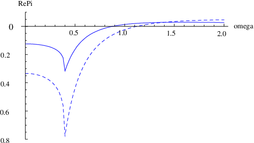
Figure 7: Real part of the self-energy Π𝐪R​(ω)\Pi^{R}_{\bf q}(\omega) for 𝐪=0{\bf q}=0; case (a) with masses m1=m2=0.2​mm_{1}=m_{2}=0.2m and temperatures T1=0.5​mT_{1}=0.5m (solid) and T2=mT_{2}=m (dashed).

In both cases the imaginary part of the self-energy is known analytically [17, 23]. The relevant formulae are collected in Appendix A.3. For m≫m1,m2m\gg m_{1},m_{2}, the decay width of Φ\Phi at zero temperature is given by

Γ=116​π​(gm)2​m.\Gamma=\frac{1}{16\pi}\left(\frac{g}{m}\right)^{2}m\ . (7.2)

To illustrate thermal effects we shall use a rather large coupling which corresponds to Γ/m=0.1\Gamma/m=0.1.

The spectral function ρ𝐪​(ω)\rho_{\bf q}(\omega) (cf. (4.15)) is shown in Figures 4 and 5 for the two mass patterns (a) and (b), respectively. In case (a), Π𝐪R\Pi^{R}_{\bf q} has an imaginary part at zero temperature. The width is large, and already at small temperatures the quasi-particle profile becomes broad. On the contrary, in case (b) the zero-temperature width is zero and the finite-temperature width is small. Hence, the quasi-particle profile becomes broad only at much larger temperatures. The spectral function Δ𝐪−​(y)\Delta^{-}_{\bf q}(y) is the Fourier transform of i​ρ𝐪​(ω)i\rho_{\bf q}(\omega). As Figure 6 illustrates, it approximately represents a damped oscillation with frequency Ω𝐪\Omega_{\bf q} and damping rate Γ𝐪\Gamma_{\bf q}.

It is interesting that thermal corrections can increase or decrease the particle mass mm. Whether the quasi-particle peak moves to the right or to the left depends on the position of the zero-temperature pole relative to the branch cuts, and it also depends on the temperature. This can be seen by considering the real part of the self-energy, which is displayed for two different temperatures in Fig. 7 for case (a). For the smaller temperature one has Re⁡Π𝐪=𝟎R​(m)>0\re\Pi^{R}_{\bf q=0}(m)>0, whereas Re⁡Π𝐪=𝟎R​(m)<0\re\Pi^{R}_{\bf q=0}(m)<0 holds for the larger temperature, which corresponds to a shift of the particle mass to the right and to the left, respectively.

The statistical propagator Δ𝐪+​(t1,t2)\Delta^{+}_{\bf q}(t_{1},t_{2}) depends on the initial conditions. The most general gaussian initial density matrix has five free parameters (cf. [13]). We consider the simplest case of a free field density matrix and vanishing mean values Φ\Phi and Φ˙\dot{\Phi}, which implies for each momentum mode,

Φ𝐪,in\displaystyle\Phi_{\bf q,\text{in}} =0,\displaystyle=0\ , (7.3)
Φ˙𝐪,in\displaystyle\dot{\Phi}_{\bf q,\text{in}} =0,\displaystyle=0\ , (7.4)
Δ𝐪,in+\displaystyle\Delta^{+}_{\bf q,\text{in}} =Δ𝐪+​(t1,t2)|t1=t2=0=1ω𝐪​(12+n𝐪),\displaystyle=\Delta^{+}_{\bf q}(t_{1},t_{2})|_{t_{1}=t_{2}=0}=\frac{1}{\omega_{\bf q}}\left(\frac{1}{2}+n_{\bf q}\right)\ , (7.5)
Δ˙𝐪,in+\displaystyle\dot{\Delta}^{+}_{\bf q,\text{in}} =∂t1Δ𝐪+​(t1,t2)|t1=t2=0=∂t2Δ𝐪+​(t1,t2)|t1=t2=0=0,\displaystyle=\partial_{t_{1}}\Delta^{+}_{\bf q}(t_{1},t_{2})|_{t_{1}=t_{2}=0}=\partial_{t_{2}}\Delta^{+}_{\bf q}(t_{1},t_{2})|_{t_{1}=t_{2}=0}=0\ , (7.6)
Δ¨𝐪,in+\displaystyle\ddot{\Delta}^{+}_{\bf q,\text{in}} =∂t1∂t2Δ𝐪+​(t1,t2)|t1=t2=0=ω𝐪​(12+n𝐪).\displaystyle=\partial_{t_{1}}\partial_{t_{2}}\Delta^{+}_{\bf q}(t_{1},t_{2})|_{t_{1}=t_{2}=0}=\omega_{\bf q}\left(\frac{1}{2}+n_{\bf q}\right)\ . (7.7)

The initial state of the system is now characterized by only one parameter n𝐪n_{\bf q} which corresponds to an initial number density for a free field.

Refer to caption
Figure 8: Statistical propagator Δ𝐪+​(t1,t2)\Delta^{+}_{\bf q}(t_{1},t_{2}) for 𝐪=0{\bf q}=0; case (b) with masses m1=mm_{1}=m, m2=5​mm_{2}=5m and T=10​mT=10m.
Refer to caption
Figure 9: Statistical propagator Δ𝐪+​(t1,t2)\Delta_{\bf q}^{+}(t_{1},t_{2}) as function of y=t1−t2y=t_{1}-t_{2} for 𝐪=0{\bf q}=0; case (b) with m1=mm_{1}=m, m2=5​mm_{2}=5m, T=10​mT=10m and three values of t=(t1+t2)/2t=(t_{1}+t_{2})/2: m​t=15mt=15 (dashed line), m​t=20mt=20 (dotted-dashed), m​t=60mt=60 (solid).
Refer to caption
Figure 10: Statistical propagator Δ𝐪+​(t1,t2)\Delta_{\bf q}^{+}(t_{1},t_{2}) as function of t=(t1+t2)/2t=(t_{1}+t_{2})/2 for y=0y=0, 𝐪=0{\bf q}=0; case (b) with masses m1=mm_{1}=m, m2=5​mm_{2}=5m and T=10​mT=10m.
Refer to caption
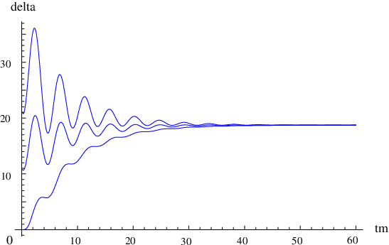
Figure 11: Statistical propagator Δ𝐪+​(t1,t2)\Delta_{\bf q}^{+}(t_{1},t_{2}) with q=0\textbf{q}=0 as function of t=(t1+t2)/2t=(t_{1}+t_{2})/2 for y=0y=0 and different initial conditions; case (b) with masses 𝐪=0{\bf q}=0, m1=mm_{1}=m, m2=5​mm_{2}=5m and T=10​mT=10m.

The general solution (4.28) for the statistical propagator Δ𝐪+​(t1,t2)\Delta^{+}_{\bf q}(t_{1},t_{2}) is shown in Figure 8. For fixed t=(t1+t2)/2t=(t_{1}+t_{2})/2 one sees damped oscillations in y=t1−t2y=t_{1}-t_{2}. The amplitude increases with increasing time tt, as illustrated by Figure 9. For fixed y=t1−t2y=t_{1}-t_{2} one observes the approach to equilibrium with increasing t=(t1+t2)/2t=(t_{1}+t_{2})/2. For large times the departure from equilibrium is described by a first-order differential equation, and it decreases exponentially. At small times the evolution is governed by a second-order differential equation, which leads to the oscillations visible in Figure 10. The independence of the equilibrium solution from the initial conditions is illustrated by Figure 11. The memory of the initial conditions is lost at times t>1/Γt>1/\Gamma.

Refer to caption
Figure 12: Energy density ϵ^𝐪=ϵ𝐪/ω𝐪\hat{\epsilon}_{\bf q}=\epsilon_{\bf q}/\omega_{\bf q} as function of temperature for 𝐪=0{\bf q}=0; case (b) with masses m1=mm_{1}=m, m2=5​mm_{2}=5m: total energy density (solid), particle and quasi-particle energy densities (dotted), and ’vacuum’ energy density (dashed).

Finally, it is important to recall that the equilibrium value of the energy differs from the one obtained in the Boltzmann approximation. This is illustrated in Figure 12 where the different contributions to the energy are compared as functions of temperature. For the chosen parameters the particle and quasi-particle energies are indistinguishable. The ‘vacuum contribution’ is positive, which means that the total energy is larger than the particle/quasi-particle one. The reason is that for the chosen parameters thermal corrections decrease the particle mass. For other parameter choices the ‘vacuum contribution’ can have opposite sign.

8 Conclusions and outlook

We have studied the approach to equilibrium for a real scalar field coupled to a large thermal bath. We have computed the exact two-point functions, the spectral function and the statistical propagator, for arbitrary initial conditions. This is possible for a thermal bath with many degrees of freedom such that the backreaction of the scalar field can be neglected.

The self-energy representing the thermal bath is time-translation invariant. We have shown that this is also the case for the spectral function, whereas the statistical propagator depends on two time coordinates, t1t_{1} and t2t_{2}, and also the time tit_{i} where the initial conditions are specified.

We have obtained the two-point functions by solving the Kadanoff-Baym equations, which turned out to be equivalent to solving a stochastic Langevin equation. As expected, the relaxation time is determined by the imaginary part of the self-energy, i.e., a ‘quasi-particle width’ Γ\Gamma. For t>1/Γt>1/\Gamma, the statistical propagator becomes independent of the initial conditions. It is then given by a memory integral which depends on the real and imaginary part of the self-energy.

As long as thermal corrections are small, the approach to equilibrium is well described by the ordinary Boltzmann equation, which is a local, first-order differential equation in time for the particle number density. However, in the case of large thermal corrections the notion of number density becomes ambiguous, and it is important to consider the second-order Kadanoff-Baym equations for the two-point functions rather than a Boltzmann equation. Still, as long as the quasi-particle decay width is small compared to the quasi-particle energy, a Boltzmann equation for quasi-particles describes the approach to equilibrium to good approximation. For large decay width the dynamics becomes nonlocal in time and the Boltzmann approximation breaks down.

It is interesting to study the contribution of the thermalized scalar field to energy density and pressure. For a free field these observables are determined by the Bose-Einstein distribution function. Interaction with the thermal bath can significantly modify energy density and pressure, and therefore the equation of state. The Bose-Einstein distribution as function of the complex quasi-particle pole is now the relevant quantity. Energy density and pressure differ from the expressions for a free gas of quasi-particles by a temperature-dependent ‘vacuum term’ which can become important at high temperatures.

We have illustrated these results for a toy model where the thermal bath consists of two massive scalar fields. We have considered two cases where equilibration takes place either via decays and inverse decays or via ‘Landau damping’. In general, one has to study the Kadanoff-Baym equation for the statistical propagator which depends on two time coordinates as well as initial conditions. However, for large times, t≫1/Γt\gg 1/\Gamma, the time evolution is well described by the Boltzmann equation for quasi-particles.

Our analysis has been motivated by the need of a full quantum mechanical description of leptogenesis. To achieve this, one has to consider correlation functions rather than number densities, although for parts of the calculation the use of Boltzmann equations will be sufficient. The heavy Majorana neutrino is very weakly coupled to the thermal bath. Hence, thermal corrections to its mass and width are small, and its approach to equilibrium is well described by Boltzmann equations. However, to study the dependence of the final baryon asymmetry on initial conditions it may be necessary to consider the statistical propagator, since leptogenesis takes place at tB∼1/Γt_{B}\sim 1/\Gamma. Furthermore, for lepton and Higgs fields, which have strong gauge interactions, finite-width effects can be important. At present it is unclear how accurately the leptogenesis process can be described based on a quasi-particle picture for the standard model particles which form the thermal bath. These questions are currently under investigation [24].

Acknowledgements

We would like to thank J. Berges, D. Bödeker, J. Schmidt and C. Wetterich for helpful discussions.

Appendix A The spectral function

A.1 Time-translation invariance

In this section we shall prove that the most general solution of the first Kadanoff-Baym equation is time-translation invariant. The starting point is Eq. (2.29) with the boundary conditions (2.31) - (2.33). Performing the change of variables t1=t+y/2t_{1}=t+y/2, t2=t−y/2t_{2}=t-y/2, Eq. (2.29) becomes

(14∂t2+∂t∂y+∂y2+ω𝐪2)Δ𝐪−(t;y)+∫0ydy′Π𝐪−(y−y′)Δ𝐪−(t′;y′)=0,\left(\frac{1}{4}\partial^{2}_{t}+\partial_{t}\partial_{y}+\partial^{2}_{y}+\omega_{\bf q}^{2}\right)\Delta_{\bf q}^{-}(t;y)+\int_{0}^{y}dy^{\prime}\Pi_{\bf q}^{-}(y-y^{\prime})\Delta_{\bf q}^{-}(t^{\prime};y^{\prime})=0\ , (A.1)

where t′=t−(y−y′)/2t^{\prime}=t-(y-y^{\prime})/2 and ω𝐪2=𝐪2+m2\omega_{\bf q}^{2}={\bf q}^{2}+m^{2}. Note that Δ𝐪−\Delta_{\bf q}^{-} and Π𝐪−\Pi^{-}_{\bf q} only depend on |𝐪||{\bf q}| because of rotational invariance. Both functions are antisymmetric in yy. The boundary conditions (2.31) - (2.33) read

Δ𝐪−​(t,0)\displaystyle\Delta^{-}_{\bf q}(t;0) =0,\displaystyle=0\ , (A.2)
∂tΔ𝐪−​(t,0)\displaystyle\partial_{t}\Delta^{-}_{\bf q}(t;0) =0,\displaystyle=0\ , (A.3)
∂yΔ𝐪−​(t,y)|y=0\displaystyle\partial_{y}\Delta^{-}_{\bf q}(t;y)|_{y=0} =1,\displaystyle=1\ , (A.4)
(14∂t2−∂y2)Δ𝐪−(t;y)|y=0\displaystyle\left(\frac{1}{4}\partial_{t}^{2}-\partial_{y}^{2}\right)\Delta^{-}_{\bf q}(t;y)|_{y=0} =0.\displaystyle=0\ . (A.5)

The condition (A.2) is automatically fulfilled because of the antisymmetry in yy.

To prove that Δ−\Delta^{-} is time-translation invariant we now perform an expansion in powers of Π−\Pi^{-},

Δ𝐪−=∑n=0∞Δ𝐪(n),Δ𝐪(n)=𝒪⁡(Π𝐪(n)).\Delta^{-}_{\bf q}=\sum_{n=0}^{\infty}\Delta^{(n)}_{\bf q}\ ,\quad\Delta^{(n)}_{\bf q}=\mathcal{O}(\Pi_{\bf q}^{(n)})\ . (A.6)

For n=0n=0 one has

(14∂t2+∂t∂y+∂y2+ω𝐪2)Δ𝐪(0)(t;y)=0.\left(\frac{1}{4}\partial^{2}_{t}+\partial_{t}\partial_{y}+\partial^{2}_{y}+\omega_{\bf q}^{2}\right)\Delta_{\bf q}^{(0)}(t;y)=0\ . (A.7)

Using the antisymmetry of Δ𝐪−\Delta^{-}_{\bf q} in yy, one obtains

∂t∂yΔ𝐪(0)​(t,y)=0,\partial_{t}\partial_{y}\Delta^{(0)}_{\bf q}(t;y)=0\ , (A.8)

which has the general solution

Δ𝐪(0)=a𝐪(0)​(t)+b𝐪(0)​(y).\Delta_{\bf q}^{(0)}=a^{(0)}_{\bf q}(t)+b^{(0)}_{\bf q}(y)\ . (A.9)

Every solution of Eqs. (A.7) and (A.8) satisfies the boundary condition (A.5). The condition (A.3) implies

∂tΔ𝐪(0)​(t,0)=∂ta𝐪(0)​(t)=0.\partial_{t}\Delta_{\bf q}^{(0)}(t;0)=\partial_{t}a^{(0)}_{\bf q}(t)=0\ . (A.10)

Hence, a𝐪(0)a^{(0)}_{\bf q} is constant and Δ𝐪(0)\Delta_{\bf q}^{(0)} only depends on yy. Eq. (A.7) now becomes

(∂y2+ω𝐪2)Δ𝐪(0)(y)=0,\left(\partial^{2}_{y}+\omega_{\bf q}^{2}\right)\Delta_{\bf q}^{(0)}(y)=0\ , (A.11)

which has the antisymmetric solution

Δ𝐪(0)​(y)=c𝐪(0)​sin⁡(ω𝐪​y).\Delta^{(0)}_{\bf q}(y)=c^{(0)}_{\bf q}\sin(\omega_{\bf q}y)\ . (A.12)

For n≠0n\neq 0 one can use the recurrence relation

(14∂t2+∂t∂y+∂y2+ω𝐪2)Δ𝐪(n+1)(t;y)+∫0ydy′Π𝐪−(y−y′)Δ𝐪(n)(y′)=0.\left(\frac{1}{4}\partial^{2}_{t}+\partial_{t}\partial_{y}+\partial^{2}_{y}+\omega_{\bf q}^{2}\right)\Delta_{\bf q}^{(n+1)}(t;y)+\int_{0}^{y}dy^{\prime}\Pi_{\bf q}^{-}(y-y^{\prime})\Delta_{\bf q}^{(n)}(y^{\prime})=0\ . (A.13)

Using the antisymmetry of Π𝐪−\Pi^{-}_{\bf q} and Δ𝐪−\Delta^{-}_{\bf q} in yy, one again finds

∂t∂yΔ𝐪(n+1)​(t,y)=0.\partial_{t}\partial_{y}\Delta^{(n+1)}_{\bf q}(t;y)=0\ . (A.14)

Repeating the same steps as for Δ𝐪(0)\Delta^{(0)}_{\bf q} yields the result that also Δ𝐪(n+1)\Delta^{(n+1)}_{\bf q} is independent of tt.

We conclude that the spectral function is the antisymmetric solution of the equation

(∂y2+ω𝐪2)Δ𝐪−(y)+∫0ydy′Π𝐪−(y−y′)Δ𝐪−(y′)=0,\left(\partial^{2}_{y}+\omega_{\bf q}^{2}\right)\Delta_{\bf q}^{-}(y)+\int_{0}^{y}dy^{\prime}\Pi_{\bf q}^{-}(y-y^{\prime})\Delta_{\bf q}^{-}(y^{\prime})=0\ , (A.15)

with the boundary condition

∂yΔ𝐪−​(y)|y=0=1.\partial_{y}\Delta^{-}_{\bf q}(y)|_{y=0}=1\ . (A.16)

A.2 Conventions for propagators and self-energies

In thermal equilibrium the retarded and advanced propagators and self-energies only depend on the time difference y=t1−t2y=t_{1}-t_{2}. In the following we list several relations between their Fourier transforms, which are used in the different sections. In principle, these relations are all well know, but their specific form depends on the chosen conventions. All relations are not affected by the three-dimensional Fourier transform. We therefore drop the argument 𝐪{\bf q} or 𝐱{\bf x}.

Propagators:

Δ−​(ω)∗\displaystyle\Delta^{-}(\omega)^{*} =\displaystyle= −Δ−​(ω),\displaystyle-\Delta^{-}(\omega)\ , (A.17)
Δ+​(ω)∗\displaystyle\Delta^{+}(\omega)^{*} =\displaystyle= Δ+​(ω),\displaystyle\Delta^{+}(\omega)\ , (A.18)
ΔA​(ω)\displaystyle\Delta^{A}(\omega) =\displaystyle= i2​Δ−​(ω)−𝒫​∫−∞∞d​ω′2​π​Δ−​(ω′)ω′−ω,\displaystyle\frac{i}{2}\Delta^{-}(\omega)-\mathcal{P}\int_{-\infty}^{\infty}\frac{d\omega^{\prime}}{2\pi}\frac{\Delta^{-}(\omega^{\prime})}{\omega^{\prime}-\omega}\ , (A.19)
ΔR​(ω)\displaystyle\Delta^{R}(\omega) =\displaystyle= −i2​Δ−​(ω)−𝒫​∫−∞∞d​ω′2​π​Δ−​(ω′)ω′−ω,\displaystyle-\frac{i}{2}\Delta^{-}(\omega)-\mathcal{P}\int_{-\infty}^{\infty}\frac{d\omega^{\prime}}{2\pi}\frac{\Delta^{-}(\omega^{\prime})}{\omega^{\prime}-\omega}\ , (A.20)
Re⁡ΔA​(ω)\displaystyle\re\Delta^{A}(\omega) =\displaystyle= −Re⁡ΔR​(ω)=i2​Δ−​(ω),\displaystyle-\re\Delta^{R}(\omega)=\frac{i}{2}\Delta^{-}(\omega)\ , (A.21)
Im⁡ΔA​(ω)\displaystyle\im\Delta^{A}(\omega) =\displaystyle= ImΔR(ω)=−𝒫∫−∞∞d​ω′2​π​iΔ−​(ω′)ω′−ω,\displaystyle\im\Delta^{R}(\omega)=-\mathcal{P}\int_{-\infty}^{\infty}\frac{d\omega^{\prime}}{2\pi i}\frac{\Delta^{-}(\omega^{\prime})}{\omega^{\prime}-\omega}\ , (A.22)
ΔA​(−ω)\displaystyle\Delta^{A}(-\omega) =\displaystyle= ΔR​(ω).\displaystyle\Delta^{R}(\omega)\ . (A.23)

Self-energies:

Π−​(ω)∗\displaystyle\Pi^{-}(\omega)^{*} =\displaystyle= −Π−​(ω),\displaystyle-\Pi^{-}(\omega)\ , (A.25)
Π+​(ω)∗\displaystyle\Pi^{+}(\omega)^{*} =\displaystyle= Π+​(ω),\displaystyle\Pi^{+}(\omega)\ , (A.26)
ΠA​(ω)\displaystyle\Pi^{A}(\omega) =\displaystyle= −12​Π−​(ω)+𝒫​∫d​ω′2​π​i​Π−​(ω′)ω′−ω,\displaystyle-\frac{1}{2}\Pi^{-}(\omega)+\mathcal{P}\int\frac{d\omega^{\prime}}{2\pi i}\frac{\Pi^{-}(\omega^{\prime})}{\omega^{\prime}-\omega}\ , (A.27)
ΠR​(ω)\displaystyle\Pi^{R}(\omega) =\displaystyle= 12​Π−​(ω)+𝒫​∫d​ω′2​π​i​Π−​(ω′)ω′−ω,\displaystyle\frac{1}{2}\Pi^{-}(\omega)+\mathcal{P}\int\frac{d\omega^{\prime}}{2\pi i}\frac{\Pi^{-}(\omega^{\prime})}{\omega^{\prime}-\omega}\ , (A.28)
Re⁡ΠA​(ω)\displaystyle\re\Pi^{A}(\omega) =\displaystyle= Re⁡ΠR​(ω)=𝒫​∫d​ω′2​π​i​Π−​(ω′)ω′−ω,\displaystyle\re\Pi^{R}(\omega)=\mathcal{P}\int\frac{d\omega^{\prime}}{2\pi i}\frac{\Pi^{-}(\omega^{\prime})}{\omega^{\prime}-\omega}\ , (A.29)
Im⁡ΠA​(ω)\displaystyle\im\Pi^{A}(\omega) =\displaystyle= −Im⁡ΠR​(ω)=i2​Π−​(ω),\displaystyle-\im\Pi^{R}(\omega)=\frac{i}{2}\Pi^{-}(\omega)\ , (A.30)
ΠA​(−ω)\displaystyle\Pi^{A}(-\omega) =\displaystyle= ΠR​(ω).\displaystyle\Pi^{R}(\omega)\ . (A.31)

A.3 Scalar field model

The interaction with the thermal bath changes the spectral function of a free scalar particle,

ρ𝐪​(ω)=2​π​sign​(ω)​δ​(ω2−ω𝐪2),\rho_{\bf q}(\omega)=2\pi\text{sign}(\omega)\delta(\omega^{2}-\omega_{\bf q}^{2})\ , (A.32)

to the expression (4.15) which depends on real and imaginary part of the self-energy,

ρ𝐪​(ω)=−2​Im​Π𝐪R​(ω)+2​ω​ϵ[ω2−ω𝐪2−Re​Π𝐪R​(ω)]2+[Im​Π𝐪R​(ω)+ω​ϵ]2.\rho_{\bf q}(\omega)={-2{\rm Im}\Pi^{R}_{\bf q}(\omega)+2\omega\epsilon\over[\omega^{2}-\omega_{\bf q}^{2}-{\rm Re}\Pi^{R}_{\bf q}(\omega)]^{2}+[{\rm Im}\Pi^{R}_{\bf q}(\omega)+\omega\epsilon]^{2}}\ . (A.33)

We have computed the imaginary part of the self-energy in the scalar field model defined in Section 7, assuming free thermal propagators for the fields χ1\chi_{1} and χ2\chi_{2}. The result agrees with [17]. One obtains (q=(ω𝐪,𝐪)q=(\omega_{\bf q},\bf q)):

−Im⁡Π𝐪R​(ω)=σ0​(q)+σβ(a)​(q)+σβ(b)​(q).-\im\Pi^{R}_{\bf q}(\omega)=\sigma_{0}(q)+\sigma^{(a)}_{\beta}(q)+\sigma^{(b)}_{\beta}(q)\ . (A.34)

Here σ0\sigma_{0} is the zero-temperature contribution due to the decay process Φ→χ1​χ2\Phi\rightarrow\chi_{1}\chi_{2},

σ0​(q)=\displaystyle\sigma_{0}(q)= g216​π​q2​sign​(ω)​Θ​(q2−(m1+m2)2)\displaystyle\frac{g^{2}}{16\pi q^{2}}\text{sign}(\omega)\Theta(q^{2}-(m_{1}+m_{2})^{2})
×((q2)2−2​q2​(m12+m22)+(m12−m22)2)12,\displaystyle\times\left((q^{2})^{2}-2q^{2}(m_{1}^{2}+m_{2}^{2})+(m_{1}^{2}-m_{2}^{2})^{2}\right)^{\frac{1}{2}}\ , (A.35)

σβ(a)\sigma^{(a)}_{\beta} is the finite-temperature contribution from this process,

σβ(a)​(q)=\displaystyle\sigma^{(a)}_{\beta}(q)= g216​π|𝐪|β​sign​(ω)​Θ​(q2−(m1+m2)2)\displaystyle\frac{g^{2}}{16\pi|\bf q|\beta}\text{sign}(\omega)\Theta(q^{2}-(m_{1}+m_{2})^{2})
×(ln⁡(1−e−β​ω+1−e−β​ω−)+(m1↔m2)),\displaystyle\times\left(\ln\left(\frac{1-e^{-\beta\omega_{+}}}{1-e^{-\beta\omega_{-}}}\right)+(m_{1}\leftrightarrow m_{2})\right)\ , (A.36)

and σβ(b)​(𝐪)\sigma^{(b)}_{\beta}(\bf q) is the finite-temperature contribution from processes χi→χj​ϕ\chi_{i}\rightarrow\chi_{j}\phi,33 3 Note that we disagree with the discussion in [22] which implies the additional factor Θ⁡(|m12−m22|−q2)\Theta(|m_{1}^{2}-m_{2}^{2}|-q^{2}).

σβ(b)​(q)=\displaystyle\sigma^{(b)}_{\beta}(q)= g216​π|𝐪|β​sign​(ω)​Θ​((m1−m2)2−q2)\displaystyle\frac{g^{2}}{16\pi|\bf q|\beta}\text{sign}(\omega)\Theta((m_{1}-m_{2})^{2}-q^{2})
×(ln⁡(1−e−β​|ω−|1−e−β​|ω+|)+(m1↔m2)),\displaystyle\times\left(\ln\left(\frac{1-e^{-\beta|\omega_{-}|}}{1-e^{-\beta|\omega_{+}|}}\right)+(m_{1}\leftrightarrow m_{2})\right)\ , (A.37)

where we have used the abbreviations

ω±=|ω|2​q2​(q2+m12−m22)±|q|2​|q2|​((q2+m12−m22)2−4​q2​m12)12.\omega_{\pm}=\frac{|\omega|}{2q^{2}}(q^{2}+m_{1}^{2}-m_{2}^{2})\pm\frac{|\textbf{q}|}{2|q^{2}|}\left((q^{2}+m_{1}^{2}-m_{2}^{2})^{2}-4q^{2}m_{1}^{2}\right)^{\frac{1}{2}}\ . (A.38)

The real part of the self-energy can be computed using the dispersion relation relation,

Re⁡Π𝐪R​(ω)=1π​𝒫​∫−∞∞d​ω′​Im⁡Π𝐪R​(ω′)ω′−ω.\re\Pi^{R}_{\bf q}(\omega)=\frac{1}{\pi}\mathcal{P}\int_{-\infty}^{\infty}d\omega^{\prime}\frac{\im\Pi^{R}_{\bf q}(\omega^{\prime})}{\omega^{\prime}-\omega}\ . (A.39)
Refer to caption
Figure 13: Poles and cuts of the spectral function ρ⁡(ω)\rho(\omega) for q=0\textbf{q}=0 at T=0T=0: (a) m>m1+m2m>m_{1}+m_{2}, and (b) m<m1+m2m<m_{1}+m_{2}.

Based on these expressions we can discuss the analytic structure of the spectral function. For a free field ρ𝐪​(ω)\rho_{\bf q}(\omega) is given by (A.32) which has two poles at ω=±ωq\omega=\pm\omega_{q} in the complex ω\omega-plane. The interaction of Φ\Phi with χ1\chi_{1} and χ2\chi_{2} does not modify these poles for m<m1+m2m<m_{1}+m_{2}, where Φ\Phi is stable at zero temperature. In addition there are branch cuts at the two-particle thresholds |ω|>ωth​1=𝐪2+(m1+m2)2|\omega|>\omega_{\text{th}1}=\sqrt{{\bf q}^{2}+(m_{1}+m_{2})^{2}} (see Fig. 13bb). They correspond to virtual decays and inverse decays, Φ↔χ​χ\Phi\leftrightarrow\chi\chi. In the case m>m1+m2m>m_{1}+m_{2} these processes can happen on-shell since m>ωth​1m>\omega_{\text{th}1}, and Φ\Phi becomes unstable. Now the spectral function has four poles in the complex ω\omega-plane, whose real parts lie in the region of the branch cuts (see Fig. 13aa). The imaginary parts of the poles correspond to the decay width of Φ\Phi.

The analytic structure of the spectral function at finite temperature is displayed in Fig. 14. The position of ωth​1\omega_{\text{th}1} is shifted due to thermal corrections from Re⁡Π𝐪R\re\Pi^{R}_{\bf q}. Furthermore, a new branch cut appears in the region where σb≠0\sigma_{b}\neq 0, i.e. for |ω|<ωth​2=𝐪2+(m1−m2)2|\omega|<\omega_{\text{th}2}=\sqrt{{\bf q}^{2}+(m_{1}-m_{2})^{2}}. This is due to processes χ↔ϕ​χ\chi\leftrightarrow\phi\chi and corresponds to Landau damping of quasi-particles in the plasma. If the real part of the poles falls into the regions of one of the branch cuts, i.e. |ω|<ωth​2|\omega|<\omega_{\text{th}2} or |ω|>ωth​1|\omega|>\omega_{\text{th}1}, they acquire an imaginary part which corresponds to the quasi-particle decay width (see Fig. 14).

Refer to caption
Figure 14: Poles and cuts of the spectral function ρ⁡(ω)\rho(\omega) for q=0\textbf{q}=0 at T≠0T\neq 0: (a) m>m1+m2m>m_{1}+m_{2}, and (b) m<m1+m2m<m_{1}+m_{2}.

Qualitatively, this analytic structure is typical for interacting quantum field theories at finite temperature. In general, the spectral function can have additional singular contributions for m<|ω|<ωth​1m<|\omega|<\omega_{\text{th}1} corresponding to bound states. At finite temperature they are also dressed to quasi-particles.

A.4 Breit-Wigner approximation

In the regime of couplings and temperatures where |Im⁡Π𝐪R​(Ω𝐪)|≪Ω𝐪2|\im\Pi^{R}_{\bf q}(\Omega_{\bf q})|\ll\Omega_{\bf q}^{2}, so that the quasi-particle picture holds, one can approximate the spectral function ρ𝐪​(ω)\rho_{\bf q}(\omega) by a Breit-Wigner function. From the expression (4.15) one easily obtains

ρ𝐪​(ω)≃Z𝐪2​Ω𝐪​sign​(ω)​Γ𝐪(|ω|−Ω𝐪)2+14​Γ𝐪2,\rho_{\bf q}(\omega)\simeq\frac{Z_{\bf q}}{2\Omega_{\bf q}}\frac{\text{sign}(\omega)\Gamma_{\bf q}}{\left(|\omega|-\Omega_{\bf q}\right)^{2}+\frac{1}{4}\Gamma_{\bf q}^{2}}\ , (A.40)

where Γ𝐪\Gamma_{\bf q} is the quasi-particle width

Γ𝐪=−Z𝐪​Im⁡Π𝐪R​(Ω𝐪)Ω𝐪,\Gamma_{\bf q}=-Z_{\bf q}\frac{{\im}\Pi^{R}_{\bf q}(\Omega_{\bf q})}{\Omega_{\bf q}}\ , (A.41)

with

Z𝐪=(1−12​Ω𝐪​∂Re⁡Π𝐪R​(ω)∂ω|ω=Ω𝐪)−1.Z_{\bf q}=\left(1-\frac{1}{2\Omega_{\bf q}}\frac{\partial{\re}\Pi^{R}_{\bf q}(\omega)}{\partial\omega}\Big|_{\omega=\Omega_{\bf q}}\right)^{-1}\ . (A.42)

Contrary to the exact spectral function (4.15), the Breit-Wigner approximation (A.40) has no branch cuts. The integrals over ω\omega are dominated by the regions around the quasi-particle poles where the two functions are very similar. For the Fourier transform, the spectral function in real time, one obtains

Δ𝐪−(y)≃Z𝐪sin⁡(Ωq​y)Ω𝐪e−Γqt/2.\Delta^{-}_{\bf q}(y)\simeq Z_{\bf q}\frac{\sin(\Omega_{q}y)}{\Omega_{\bf q}}e^{-\Gamma_{q}t/2}\ . (A.43)

References

  • [1] E. W. Kolb and M. S. Turner, The Early Universe, Addison-Wesley, New York, 1990.
  • [2] V. Mukhanov, Physical Foundations of Cosmology, Cambridge University Press, Cambridge, 2005.
  • [3] M. Fukugita and T. Yanagida, Phys. Lett. B 174 (1986) 45.
  • [4] M. A. Luty, Phys. Rev. D 45 (1992) 455;
    L. Covi, E. Roulet and F. Vissani, Phys. Lett. B 384 (1996) 169 [hep-ph/9605319];
    W. Buchmuller and M. Plumacher, Phys. Lett. B 389 (1996) 73 [hep-ph/9608308].
  • [5] For reviews and references, see
    W. Buchmuller, R. D. Peccei and T. Yanagida, Ann. Rev. Nucl. Part. Sci. 55 (2005) 311 [hep-ph/0502169];
    S. Davidson, E. Nardi and Y. Nir, Phys. Rept. 466 (2008) 105 [arXiv:0802.2962].
  • [6] W. Buchmuller and S. Fredenhagen, Phys. Lett. B 483 (2000) 217 [hep-ph/0004145].
  • [7] M. Lindner and M. M. Muller, Phys. Rev. D 73 (2006) 125002 [hep-ph/0512147]; Phys. Rev. D 77, 025027 (2008) [arXiv:0710.2917].
  • [8] A. De Simone and A. Riotto, JCAP 0708 (2007) 002 [hep-ph/0703175].
  • [9] R. Barbieri, P. Creminelli, A. Strumia and N. Tetradis, Nucl. Phys. B 575 (2000) 61 [hep-ph/9911315];
    T. Endoh, T. Morozumi and Z. h. Xiong, Prog. Theor. Phys. 111 (2004) 123 [hep-ph/0308276];
    A. Abada, S. Davidson, F. X. Josse-Michaux, M. Losada and A. Riotto, JCAP 0604 (2006) 004 [hep-ph/0601083];
    E. Nardi, Y. Nir, E. Roulet and J. Racker, JHEP 0601 (2006) 164 [hep-ph/0601084];
    S. Blanchet, P. Di Bari and G. G. Raffelt, JCAP 0703 (2007) 012 [hep-ph/0611337].
  • [10] L. P. Kadanoff and G. Baym, Quantum Statistical Mechanics, Benjamin, New York, 1962.
  • [11] J. Schwinger, J. Math. Phys. 2 (1961) 407;
    P. M. Bakschi and K. T.  Mahanthappa, J. Math. Phys. 4 (1963) 1;
    P. M. Bakschi and K. T.  Mahanthappa, J. Math. Phys. 4 (1963) 12;
    L. V. Keldysh, Zh. Eksp. Teor. Fiz. 47 (1964) 1515 [Sov. Phys. JETP 20 (1965) 1018].
  • [12] M. Le Bellac, Thermal Field Theory, Cambridge University Press, Cambridge, 1996.
  • [13] J. Berges, Introduction to Nonequilibrium Quantum Field Theory, AIP Conf. Proc. 739 (2005) 3 [hep-ph/0409233].
  • [14] K. c. Chou, Z. b. Su, B. l. Hao and L. Yu, Phys. Rept. 118 (1985) 1.
  • [15] J. Zinn-Justin, Quantum field theory and critical phenomena, Int. Ser. Monogr. Phys. 85 (1993) 1.
  • [16] J. Yokoyama, Phys. Rev. D 70 (2004) 103511 [arXiv:hep-ph/0406072].
  • [17] D. Boyanovsky, K. Davey and C. M. Ho, Phys. Rev. D 71 (2005) 023523 [arXiv:hep-ph/0411042].
  • [18] K. Kainulainen, T. Prokopec, M. G. Schmidt and S. Weinstock, JHEP 0106 (2001) 031 [hep-ph/0105295]; Phys. Rev. D 66 (2002) 043502 [hep-ph/0202177].
  • [19] C. Greiner and S. Leupold, Annals Phys. 270 (1998) 328 [hep-ph/9802312].
  • [20] J. Berges, A. Rothkopf and J. Schmidt, Phys. Rev. Lett. 101 (2008) 041603 [arXiv:0803.0131].
  • [21] W. Buchmuller, P. Di Bari and M. Plumacher, Nucl. Phys. B 643 (2002) 367 [Erratum-ibid. B 793 (2008) 362] [hep-ph/0205349]; Nucl. Phys. B 665 (2003) 445 [hep-ph/0302092]; Annals Phys. 315 (2005) 305 [hep-ph/0401240].
  • [22] H. A. Weldon, Phys. Rev. D 28 (1983) 2007.
  • [23] M. Drewes, Thesis, DESY 2006 (unpublished)
  • [24] A. Anisimov, W. Buchmüller, M. Drewes and S. Mendizabal, in preparation.