Magnetic Bianchi I Universe in Loop Quantum Cosmology
Abstract
We examine the dynamical consequences of homogeneous cosmological magnetic fields in the framework of loop quantum cosmology. We show that a big-bounce occurs in a collapsing magnetized Bianchi I universe, thus extending the known cases of singularity-avoidance. Previous work has shown that perfect fluid Bianchi I universes in loop quantum cosmology avoid the singularity via a bounce. The fluid has zero anisotropic stress, and the shear anisotropy in this case is conserved through the bounce. By contrast, the magnetic field has nonzero anisotropic stress, and shear anisotropy is not conserved through the bounce. After the bounce, the universe enters a classical phase. The addition of a dust fluid does not change these results qualitatively.
I Introduction
Loop quantum cosmology (LQC) is a theory of quantum cosmology based on the more general theory of loop quantum gravity [1] (for reviews, see [2, 3, 4]). One of the most important predictions of LQC is the avoidance of the big-bang singularity, which is replaced by a bouncing universe [5, 6, 7, 8, 9] for isotropic models sourced by a massless scalar field. This result has been derived rigorously at the level of the quantum theory, but has also been understood at the level of approximate effective classical equations that capture the main features of the quantum dynamics.
Extending the rigorous quantum dynamics to the anisotropic Bianchi I model is challenging. Because of this, the dynamics of Bianchi I in LQC have mostly been studied by extrapolating the approximate effective semi-classical equations that proved successful in the isotropic case. For matter with zero anisotropic stress, the effective equations predict a bounce that avoids the classical singularity [10], thus extending the results of the isotropic case. Furthermore, it was shown that the shear anisotropy does not blow up in the collapsing phase, but remain finite through the bounce. Several ambiguities in the quantum construction of the Hamiltonian constraint were considered [10], one of which has since been favored by gauge considerations [11] and by a more thorough construction of the quantum theory [12]. With this choice of quantization scheme, it was shown that the anisotropic shear is in fact conserved across the bounce when the matter has zero anisotropic stress [10].
In this paper, we couple a homogeneous magnetic field to a Bianchi I universe and consider the effective semi-classical modifications to the equations of motion. We show that the singularity is still avoided via a bounce, during which anisotropies remain finite. However, the anisotropic stress in the magnetic field leads to a non-conservation of shear anisotropy through the bounce, in contrast to the case where of matter has zero anisotropic stress.
II Classical Equations
The inclusion of a cosmological magnetic field breaks isotropy, so we consider an anisotropic Bianchi cosmology, the simplest being the Bianchi I model:
| (1) |
Maxwell’s equations are
| (2) |
where is the four-current. The Faraday tensor defines electric and magnetic fields relative to observers with four-velocity [13]
| (3) |
where is the alternating tensor in the observer’s rest-space.
We assume high conductivity in the early universe, so that the electric field is effectively zero, and Maxwell’s equations reduce to
| (4) | |||||
| (5) |
where projects into the rest-space, is the volume expansion and is the shear:
| (6) |
For a homogeneous magnetic field in Bianchi I, the divergence constraint is automatically satisfied, and the curl constraint shows that there is no 3-current. To solve the induction equation (4), we assume without loss of generality that the magnetic field is aligned along the -direction: . The solution is
| (7) |
where is constant, in agreement with [14].
The electromagnetic energy-momentum tensor is given by
| (8) | |||||
where the magnetic energy density and anisotropic stress are
| (9) |
For the case with only a magnetic field, the Einstein field equations lead to [14]:
| (10) | |||||
| (11) |
where are constants. It follows that
| (12) |
and thus any expansion in the magnetic field direction will eventually come to rest at the maximum scale factor and turn around into a contracting phase. The solutions can be given analytically [14]:
| (13) | |||||
| (14) |
where the refers to the expanding (collapsing) branches before (after) is reached.
We can now analyze the singularity behavior of the general solutions. From Eq. (13), the volume goes to zero or infinity when goes to zero, depending on the value of . There are two separate cases. The first is the axisymmetric case, , . From Eqs. (13) and (14), the axisymmetric singularity is characterized by
| (15) |
Directions orthogonal to the magnetic field freeze as the singularity is approached, while the magnetic field direction contracts to zero, along with the total volume. This singularity is present in all solutions for the axisymmetric case. The overall evolution is characterized by expansion in the direction of the magnetic field until is reached. After that, the direction contracts and reaches the singularity in finite proper time. For this type of evolution, past infinity is characterized by while . In addition, the time reversed scenario is possible.
The non-axisymmetric case is slightly more complicated, but again all trajectories are singular. In this case , and the singularity is characterized by
| (16) |
and vice-versa if . Thus the singularities are again given by going to zero, with one of the orthogonal directions contracting to zero, while the other expands to infinity in such a way that still goes to zero.
III Effective Loop Quantum Equations
The loop quantum formulation is based on a Hamiltonian framework where the gravitational degrees of freedom in the Bianchi I model are encoded in three triad components and momentum components , related to the metric components as
| (17) |
where is the real-valued Barbero-Immirzi parameter and represents an ambiguity parameter of loop quantum gravity. Black hole entropy calculations can be used to fix its value. In terms of these variables, the Hamiltonian is given by
| (18) |
where is the matter contribution to the Hamiltonian. Einstein’s equations can then be derived from Hamilton’s equations, which explicitly for this system are
| (19) |
The Hamiltonian must also vanish for the system:
| (20) |
The Hamiltonian for the matter contribution is proportional to the energy density of the matter, so the magnetic Hamiltonian is given by
| (21) |
We will also consider a perfect fluid with constant equation of state . This can be added to the matter Hamiltonian by first solving the conservation equation to give
| (22) |
where is a constant.
Analyzing the system at the level of the quantum difference equations of LQC for this model would be highly challenging, given the complexity of the Bianchi I equations. We thus consider approximate semi-classical equations of motion that incorporate loop quantum modifications. These effective equations have been shown to be very good approximations for the case of isotropic cosmologies sourced by a massless scalar field [5, 6, 7, 8, 9], and the results have been extrapolated to more complicated models. The corrections modify the general relativistic Hamiltonian (18) to be of the form [10]
| (23) |
The parameters are the key ingredients determining the quantum corrections. It is easy to see that in the limit , the classical Hamiltonian (18) is recovered. The parameters are assumed to be functions of the triad components , and their precise specification is an ambiguity of the quantization. Two possible constructions are discussed in [10], although one of them has been argued to be more physical on the grounds of certain gauge invariance considerations in [11] and of a more rigorous construction of the quantum theory in [12]. We will focus on that scheme in this paper. The particular form is
| (24) |
where is a constant that is typically related to the minimum area gap of loop quantum gravity. In this paper we assume that in Planck units; the precise value will not affect the qualitative results. The effective equations of motion can be derived as in the general relativistic case, using Hamilton’s equations (19) and the vanishing of the Hamiltonian.


The equations of motion are sufficiently complicated to not allow for an analytic solution. Despite that, some general conclusions can be made from the form of the equations. First, as shown in [10], the vanishing of the Hamiltonian (23) immediately implies a bound on the energy density of the matter. This arises from the bound in the terms of the constraint. The precise bound is the same critical density that characterizes the bounce in the isotropic models:
| (25) |
The total energy density of the matter (magnetic plus fluid) must be below this value. This is an indication that the classical singularity (where the energy density diverges) is removed and replaced by a bounce. The second conclusion from the effective equations, is that if the matter has zero anisotropic stress, the shear term is conserved before and after the bounce. Since the magnetic field has non-zero anisotropic stress, Eq. (9), this behavior is not guaranteed.
In the next section, we present numerical results.
IV Numerical solution of the effective loop quantum equations


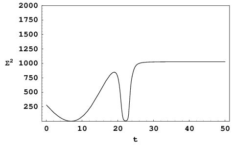
The first case is an axisymmetric spacetime () sourced only by the magnetic field. Classically, the singularity is characterized by Eq. (15). We use initial conditions corresponding to a classically collapsing universe approaching the classical singularity. The solution is shown in Fig. 1. The quantum solution matches the classical well until the singularity is approached. Then the quantum effects act repulsively – preventing from reaching zero, and leading to bounces in . The volume factor confirms that a bounce replaces the classical singularity. The post-bounce expanding universe has and , as in the classical case. Thus the quantum effects join a classical contracting branch with an expanding classical branch. The energy density shown in Fig. 1 remains bounded below the classical critical density as expected from analytical considerations. Finally, the shear energy density is shown to remain finite through the evolution, but is not conserved through the bounce. This is in contrast to the pure-fluid case [10], where shear is conserved. The difference arises from the non-zero magnetic anisotropic stress, Eq. (9), which leads to production of shear anisotropy.


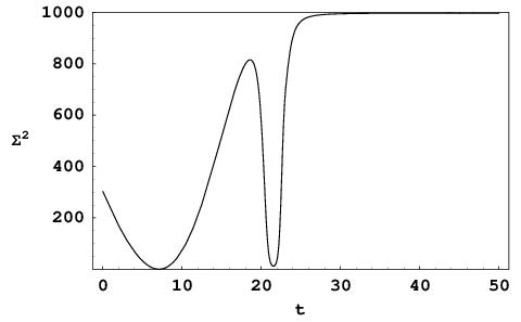

Figure 2 shows the solution for the pure-magnetic non-axisymmetric case. The classical singularity is described in Eq. (16). Once again a bounce occurs in the volume near the point of the classical singularity. With the choice of initial conditions in Fig. 2, classically while at the singularity. With the quantum effects, and are repelled from zero, and bounces. As in the axisymmetric case, the post-bounce regime is an expanding universe with expanding and contracting. The overall behavior is qualitatively similar to the axisymmetric case, and again the energy density of the magnetic field is bounded below and the shear is not conserved.
An alternative non-axisymmetric choice of initial conditions is shown in Fig. 3. The initial conditions are chosen to be in a Kasner phase, where two directions are contracting and one is expanding, while overall there is contraction in the volume. The qualitative behavior is qualitatively similar to the first non-axisymmetric example in Fig. 2.
As a final case, we included a dust perfect fluid, , with the magnetic field. We chose non-axisymmetric initial conditions with the volume collapsing. Figure 4 shows a bounce qualitatively similar to the pure-magnetic case. The shear term remains finite, but is not conserved. At late times in the post-bounce expansion phase, the dust begins to dominate the evolution and the universe isotropizes, since the ratio of the separate Hubble rates tends to one at late times.
V Conclusions
We have extended the effective LQC treatment of Bianchi I cosmologies by including a homogeneous magnetic field. We have studied dynamics using the approximate effective equations of motion that capture features of the (as yet unknown) true quantum LQC dynamics. Thus our results are approximate, and a more rigorous quantum construction would be needed to fully validate them or provide additional corrections.
The effective equations indicate that the singularity-avoiding bounce is not spoiled by the inclusion of a homogeneous magnetic field. Extending the results of [10], we showed that shear anisotropy does not blow up as the classical singularity is approached, but remains finite through the entire evolution. In contrast to the pure-fluid case [10], we showed shear is no longer conserved through the bounce, due to the anisotropic stress carried by the magnetic field. Our results indicate an interesting evolution of shear, possibly with a net generation of shear, but further study is needed to check whether this is generic. When we add a dust fluid to the magnetic field, the qualitative behavior through the bounce is unchanged. However, at late times after the bounce, the dominance of the dust ensures that the universe isotropizes, unlike the pure-magnetic case.
Acknowledgements: KV was supported by the Marie Curie Incoming International Grant M1F1-CT-2006-022239. The work of RM was supported by the UK’s STFC.
References
- [1] M. Bojowald, Living Rev. Rel. 8, 11 (2005) [arXiv:gr-qc/0601085].
- [2] A. Ashtekar and J. Lewandowski, Class. Quant. Grav. 21, R53 (2004) [arXiv:gr-qc/0404018].
- [3] C. Rovelli, Quantum Gravity, (CUP, Cambridge, 2004).
- [4] T. Thiemann, Modern canonical quantum general relativity (CUP, Cambridge, 2007).
- [5] A. Ashtekar, T. Pawlowski and P. Singh, Phys. Rev. Lett. 96, 141301 (2006) [arXiv:gr-qc/0602086].
- [6] A. Ashtekar, T. Pawlowski and P. Singh, Phys. Rev. D 73, 124038 (2006) [arXiv:gr-qc/0604013].
- [7] A. Ashtekar, T. Pawlowski and P. Singh, Phys. Rev. D 74, 084003 (2006) [arXiv:gr-qc/0607039].
- [8] A. Ashtekar, T. Pawlowski, P. Singh and K. Vandersloot, Phys. Rev. D 75, 024035 (2007) [arXiv:gr-qc/0612104].
- [9] K. Vandersloot, Phys. Rev. D 75, 023523 (2007) [arXiv:gr-qc/0612070].
- [10] D. W. Chiou and K. Vandersloot, Phys. Rev. D 76, 084015 (2007) [arXiv:0707.2548 [gr-qc]].
- [11] D. W. Chiou, Phys. Rev. D 76, 124037 (2007) [arXiv:0710.0416 [gr-qc]].
- [12] A. Ashtekar, E. Wilson-Ewing, to appear.
- [13] J. D. Barrow, R. Maartens and C. G. Tsagas, Phys. Rept. 449, 131 (2007) [arXiv:astro-ph/0611537].
- [14] K. C. Jacobs, Astrophys. J 155, 379 (1969).