Transverse field-induced effects in carbon nanotubes

The astounding range of experimental and theoretical studies performed on carbon nanotubes [1] has revealed a spectrum of physics characteristic of strongly correlated low-dimensional electronic systems [2]. The underlying graphene lattice structure of these tubes uniquely affects band structure, effective dimensionality, Coulomb interaction effects, and the quantum dot behavior exhibited by short nanotube segments. The band structure shows differing behavior depending on various factors such as chirality, applied gate potentials, boundary conditions at the tube ends and mechanical stress [3, 4]. In single-walled armchair nanotubes (SWNT) [5], which are the entities of interest here, gapless linearly dispersing modes endow the nanotube with its peculiar quantum wire properties. As described theoretically and ascertained experimentally, interactions within the modes of this effectively one-dimensional system cause it to behave as a Luttinger liquid characterized by non-Ohmic conductances [6, 7, 8, 9, 2]. Tubes placed between tunnel barriers act as quantum dots [10, 11], which, while displaying zero dimensional physics such as Coulomb blockade behavior, retain some higher dimensional traits such as hosting plasmons typical of one dimension and band degrees of freedom attributed to the underlying graphene lattice. Potentially invaluable to applications, these nanotube quantum dots have been proposed as elements of quantum devices and the quantum states of blockaded electrons have been regarded as candidates for units of quantum information [12]. In each of these aspects, the presence of applied fields can dramatically alter the nanotube’s behavior; here we present an extensive study of the effects of electric and magnetic fields applied transversally to the axis of the nanotube.

At the level of the band structure, it has been shown that a parallel magnetic field can have the striking effect of converting a metallic tube to a semiconducting one by way of inducing a gap [13], and vice-versa, an effect discernible in conductance, Coulomb blockade and scanning tunneling microscope (STM) measurements. Here, instead of a parallel field, we discuss transverse field configurations (both electric and magnetic) and the conditions under which a band gap opens up or the spectrum remains gapless in armchair SWNTs. In the latter case, we demonstrate, via band-structure calculations, simultaneous breaking of the valley degeneracy (of the two distinct Dirac points), the left-right-mover degeneracy, and the particle-hole symmetry. Moreover, the fields yield a non-negligible reduction in the Fermi velocity of conduction electrons traveling along the tube. We show that for certain configurations of fields, the ground state of the tube can even be made to carry finite current.

Transverse fields provide an excellent means of altering the ratio of interaction strength to the Fermi energy in SWNTs. This makes nanotubes potentially the only systems to date in which the associated Luttinger liquid physics can be tuned in a controlled fashion. As described in previous work, either an electric field [14] or a magnetic field [15, 16] alone suffices to change the value of the Luttinger liquid parameter from that measured in field-free environments. The magnitude of the electric fields required to bring about a significant change are well within current experimental reach [17]. Here, we find that our approach reproduces these results. We show that such a tuning of Luttinger parameters can mediate a transition from the system showing tendencies towards spin-density-wave (SDW) ordering to that of charge-density-wave (CDW) ordering. Furthermore, in addition to the tuning of the Luttinger parameter presented in previous works for the net charge density [14, 15, 16], we find that Luttinger-type interactions become manifest in modes associated with the density differences between nanotube bands as well. Thus we predict that akin to spin-charge separation, transverse fields can induce a spin-charge-band separation wherein the three degrees of freedom move at different velocities.

The above results are discussed in the case of an infinite system. For short tubes or finite length segments formed by tunnel barriers, boundary effects need to be taken into account. We find that applied fields influence multiple aspects of short nanotubes. First, fields can alter the single-particle energy level spacing of the tube. Here, we carefully account for the effect of the tube ends in the case that the left and right movers travel at different speeds. Second, the charging energies become field dependent, and third, the plasmon spectrum varies in accordance with the first two effects. We have conducted a comprehensive analysis of the short nanotube as a finite-sized Luttinger liquid and show how all three effects can be captured. Within this description, we discuss the structure of field-dependent Coulomb blockade peaks and how the presence of both electric and magnetic fields acts as a means of manipulating quantum states of the dot (the effect of a magnetic field alone has recently been discussed by Bellucci and Onorato [18]).

The outline of this paper is as follows. In section II we present the formulation and results of our band structure calculation. In section III we formulate an effective one-dimensional Hamiltonian which takes into account field effects. We bosonize this Hamiltonian, describing interaction effects in terms of Luttinger liquid physics. In section IV we investigate the various Luttinger liquid phases and the feasibility of using fields to access such phases. In section V we discuss field-tuned quantum dot physics. Finally, in section VI we present the highlights of our results and discuss their relevance to experiments.

We briefly recapitulate the band structure of an infinitely long armchair tube in the absence of any fields [4]. The electronic properties of graphene are well described by a tight-binding model in which electrons hop between nearest neighbors of the underlying hexagonal bipartite lattice (sublattices here labeled $A$ and $B$) with an associated energy (the hopping integral) of $t\approx 3$ eV. An armchair carbon nanotube can be regarded as a sheet of graphene rolled along the $(n,n)$-direction (for notation of the chirality, see e.g. Ref. [4]), denoted by $\hat{s}$. This gives rise to states of quantized momentum $k_{s}=(0,2\pi/L,...,2\pi(2n-1)/L)$ where $L=\sqrt{3}na$ is the circumference of the tube, and $a=\sqrt{3}a_{c}$ where $a_{c}\approx 0.15$ nm is the nearest carbon-carbon distance. The resulting series of one dimensional bands can be described by the wavevectors $\vec{k}=(k_{x},\frac{2\pi\ell}{L})$ where $k_{x}$ is the quasimomentum parallel to the tube’s axis and $\hbar\ell$ is the state’s angular momentum about the tube’s circumference. A convenient set of basis states is given by the following linear combination of atomic orbitals

$$|\Phi_{A/B}^{\ell}\rangle=\frac{1}{\sqrt{2n}}\sum_{\vec{R}\in A/B}e^{i\vec{k}\cdot\vec{R}}|\vec{R}\rangle,$$

(1)

where $|\vec{R}\rangle$ is the $\pi$-electronic state of the atom located at $\vec{R}$. The sum runs over the $n$ atoms in the unit cell that belong to either the A or B sublattice. At half filling, the associated dispersion has low energy excitations near the so-called Dirac points of the form $\epsilon=\pm\hbar v_{F}|k-\alpha k_{F}|$ where $v_{F}=\frac{\sqrt{3}ta}{2\hbar}\approx 8\times 10^{5}$ m/s, $k_{F}=4\pi/3a$ and $\alpha=\pm$. Thus, $k=\alpha k_{F}$ label the two inequivalent Fermi points.

The setup of interest is shown in Fig. 1. An external magnetic field is applied in the negative $y$-direction; an applied (transverse) electric field makes an angle $\chi$ with the magnetic field. These fields give rise to scalar and vector potentials

	$\displaystyle U(s)$	$\displaystyle=$	$\displaystyle|e|R\cos\left(\frac{s}{R}-\chi\right)$		(2)
	$\displaystyle\vec{A}$	$\displaystyle=$	$\displaystyle-Bz\hat{x},$		(3)

respectively ($R=L/2\pi$). The $x$-axis runs parallel to the tube’s axis and the additional coordinate $s$ measures the circumferential distance starting from the negative $y$-axis (a positive value of $s$ corresponds to a counterclockwise rotation as one looks along the $x$-axis in the positive direction).

These external potentials are easily accommodated within the tight binding approach. In Eq. (3) we have selected a gauge that is independent of $x$ and thus $k_{x}$ remains a good quantum number. The hopping matrix elements in the presence of the fields are given by

$$\langle\Phi^{\ell^{\prime}}_{A}\left|H\right|\Phi^{\ell}_{B}\rangle=-\frac{t}{2n}\sum_{\vec{R}\in B,\vec{R}^{\prime}\in A}e^{i(k\cdot R-k^{\prime}\cdot R^{\prime})+\frac{ie}{\hbar}(G_{R}-G_{R}^{\prime})}$$

(4)

where the sum runs over nearest neighbors $\vec{R}$, $\vec{R}^{\prime}$ and

$$G_{j}-G_{i}\approx\int_{0}^{1}d\lambda\ (\vec{r}_{i}-\vec{r}_{j})\cdot\vec{A}\left(\vec{r}+\lambda(\vec{r}_{i}-\vec{r}_{j})\right)$$

(5)

is the Aharonov-Bohm phase associated with the magnetic field [4]. The dimensionless parameter $b$ is given by $b=B\frac{\sqrt{3}|e|L^{2}}{4\pi^{2}\hbar}$. Numerically, for an $(n,n)$ nanotube, the magnetic field in Teslas is related to the dimensionless parameter $b$ via $B\approx 8.1\times 10^{4}\times b/n^{2}$ T. The scalar potential gives rise to an on-site potential described by the matrix element

$\displaystyle\langle\Phi^{\ell^{\prime}}_{A}\left|H\right|\Phi^{\ell}_{A}\rangle=\langle\Phi^{\ell^{\prime}}_{B}\left|H\right|\Phi^{\ell}_{B}\rangle=\frac{U}{2}e^{\pm i\chi}$

(6)

for $\ell^{\prime}=\ell\mp 1\mod n$ where $U=|e|ER/t$. The electric field strength in V/nm is related to $U$ by $E\approx 42\ U/n$ V/nm for a tube with chiral vector $(n,n)$. That these matrix elements mix states of different angular momentum has a straightforward classical analog: a charged particle on the surface of a cylinder will circulate around its circumference as a result of the applied fields

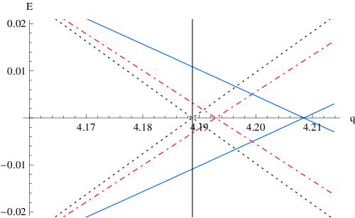
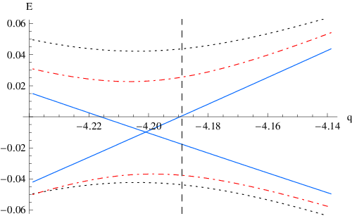
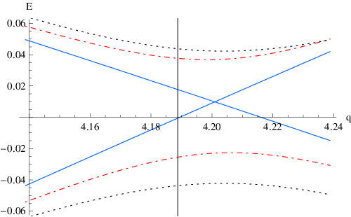
We have studied the effects of the fields perturbatively in $b$ and $U$. In the vicinity of the Fermi points, the left and right moving bands are nearly degenerate, so care must be taken in applying perturbation theory. The details of this calculation are presented in Appendix A where we carry out perturbation theory to second order. There are three cases of interest that we summarize below. An illustration of these three cases is shown in Figs. 2, 3, 4, and 5. While some of the effects discussed are rather small for standard SWNTs, we note that our band structure analysis can be applied to multi-walled nanotubes as well in which case a larger radius yields more pronounced effects.

In this section we specialize to the case of gapless modes for which interactions can be easily incorporated. As the simplest case, when only a magnetic or electric field is present, the kinetic piece of the Hamiltonian given in Eq. (13) now has $\tilde{v}_{+}=\tilde{v}_{-}\equiv\tilde{v}_{F}$ and $\epsilon_{gap}=0$, i.e.,

$$H_{0}=-i\hbar\tilde{v}_{F}\sum_{r\alpha\sigma}\int dx\ \psi^{\dagger}_{r\alpha\sigma}\partial_{x}\psi_{r\alpha\sigma}.$$

(16)

We use standard approaches such as bosonization to study the effect of fields. Where appropriate, we include discussions for the asymmetric case of $\tilde{v}_{+}\neq\tilde{v}_{-}$. We closely follow the approach of Ref. [7] whose lucid pedagogical exposition we do not repeat but instead confine our discussion to the new field-dependant features.

The presence of fields does not alter the fact that the electrons on a tube are locked into their lowest energy radial mode. Hence, it is possible to study the low energy excitations in the presence of interactions using an effective bosonized 1D Hamiltonian. Bosonization offers a great simplification since many of the quartic interaction terms in the fermionic language become quadratic once they are bosonized.

The interaction term takes the general form

$$H_{int}=\frac{1}{2}\int d\mathbf{r}\int d\mathbf{r}^{\prime}\ \Psi_{\sigma}^{\dagger}(\mathbf{r})\Psi_{\sigma^{\prime}}^{\dagger}(\mathbf{r}^{\prime})U(\mathbf{r}-\mathbf{r}^{\prime})\Psi_{\sigma^{\prime}}(\mathbf{r}^{\prime})\Psi_{\sigma}(\mathbf{r}),$$

(17)

where $\Psi_{\sigma}(\mathbf{r})$ is the field in Eq. (12) describing low-energy electrons.

Following [7], we employ the form of the Coulomb interaction on the surface of a cylinder given by

$$U(x-x^{\prime},s-s^{\prime})=\frac{e^{2}/\kappa}{\sqrt{(x-x^{\prime})^{2}+4R^{2}\sin^{2}\left(\frac{s-s^{\prime}}{2R}\right)+a_{z}^{2}}},$$

(18)

where $R$ is the radius of the tube and $x$ and $s$ the coordinates defined in the previous section and $a_{z}\approx a$ is roughly the thickness of the graphene sheet  [7]. The form of the interaction in Eq. (17) is explicitly given in terms of two-dimensional integrals. An effective interaction term involving purely linear integrals along the tube’s axis can be obtained by expressing $\Psi_{\sigma}(\mathbf{r})$ in terms of the linear and circumferential fields as in Eq. (12) and integrating out the circumferential degrees of freedom from Eq. (17). Here we remark that integration over the circumferential degrees of freedom generates field-induced terms that give rise to novel physics and can be traced to the dependence of the ground state wave function on non-zero angular momentum states in the circumferential direction.

The resulting effective interaction involves two-particle scattering processes between fermions moving along the tube axis denoted by the fields $\psi_{r\alpha\sigma}$. The associated scattering processes can be classified according to whether the incoming particles preserve their Fermi point quantum number $\alpha$ when scattered, - forward scattering ($\alpha FS$)-, or scatter across the Fermi surface - backscattering ($\alpha BS$). In Ref. [7], a further distinction is made in the forward scattering events depending on whether the interaction potential is homogeneous over the circumference of the tube ($\alpha FS0$) or is able to distinguish the microscopic differences which arise between sublattices ($\alpha FS1$). At this point, in order to obtain an effective low-energy description of the interacting electrons, the one-dimensional fermionic operators can be bosonized as in Ref. [7]:

$$\psi_{r\alpha\sigma}=\frac{\eta_{r\alpha\sigma}}{\sqrt{2\pi a_{c}}}\exp\left[i\alpha k_{F}x+i\varphi_{r\alpha\sigma}\right].$$

(19)

where

	$\displaystyle\varphi_{r\alpha\sigma}$	$\displaystyle=$	$\displaystyle\frac{\sqrt{\pi}}{2}(\phi_{c+}+r\theta_{c+}+\alpha\phi_{c-}+r\alpha\theta_{c-}$		(20)
		$\displaystyle+$	$\displaystyle\sigma\phi_{s+}+r\sigma\theta_{s+}+\alpha\sigma\phi_{c-}+r\alpha\sigma\theta_{s-}).$

The bosonic fields $\varphi$’s satisfy the commutation relations

$$[\varphi_{r\alpha\sigma}(x),\varphi_{r^{\prime}\alpha^{\prime}\sigma^{\prime}}(x^{\prime})]=-i\pi r\delta_{rr^{\prime}}\delta_{\sigma\sigma^{\prime}}{\rm sgn}(x-x^{\prime}),$$

(21)

where $r=\pm$ denotes the left- and right-movers, $\alpha=\pm$ indicates the Fermi points, and $\sigma=\pm$ represents the spin direction ($\uparrow/\downarrow$). The $\eta_{r\alpha\sigma}$’s are the so-called Klein factors; they enforce the anticommutation relations between different channels,

$$\{\eta_{r\alpha\sigma},\eta_{r^{\prime}\alpha^{\prime}\sigma^{\prime}}\}=2\delta_{rr^{\prime}}\delta_{\alpha\alpha^{\prime}}\delta_{\sigma\sigma^{\prime}}.$$

(22)

Moreover, the fields $\theta_{j\delta}(x)$’s (with $j=c/s$ and $\delta=\pm$) and their dual fields $\phi_{j\delta}(x)$ [both are linear combinations of $\varphi_{r\alpha\sigma}(x)$] in turn satisfy

$$[\phi_{j\delta}(x),\theta_{j^{\prime}\delta^{\prime}}(x^{\prime})]=-\frac{i}{2}\delta_{jj^{\prime}}\delta_{\delta\delta^{\prime}}{\rm sgn}(x-x^{\prime})$$

(23)

The effective density in a given channel takes the form

$$\widetilde{\rho}_{r\alpha\sigma}(x)=\frac{r}{2\pi}\partial_{x}\varphi_{r\alpha\sigma}(x).$$

(24)

The kinetic energy associated with the linearly dispersing fermionic modes is quadratic in the bosonized fields. As for the interactions, the dominant contributions also come from quadratic terms reflecting net density-density type interactions. As in the field-free case, the $\alpha FS0$ process has one such contribution from the usual Coulomb form involving the net charge density, which in the bosonized representation is given by

$$H_{\alpha FS,0}=\frac{2}{\pi}\int dx\ \widetilde{V}(k\approx 0)\left(\partial_{x}\theta_{c+}\right)^{2},$$

(25)

where

$$\widetilde{V}(k)\approx\frac{2e^{2}}{\kappa}\left(|\ln{kR}|+c_{0}\right)$$

(26)

is the Fourier transform of $V(x)$ and $c_{0}$ is a function of $n$ (see Eq. (B)).

The presence of either an electric or magnetic field gives rise to additional quadratic terms in the $\alpha FS0$ process . These terms have their origin in the non-zero angular momentum components of the circumferential wavefunction $\varphi_{r\alpha}(x,s)$ in Eq. (12). A detailed accounting of the radial wave functions (see appendix B) shows that an electric field contributes a term

$$H_{\alpha FS,E}=\int dx\left(\frac{2e^{2}}{\kappa}\right)\left(\frac{2}{\pi}\right)h_{1}U^{2}\left(\partial_{x}\phi_{c+}\right)^{2}$$

(27)

whereas a magnetic field provides a contribution

$$H_{\alpha FS,B}=\int dx\left(\frac{2e^{2}}{\kappa}\right)\left(\frac{2}{\pi}\right)h_{2}b^{2}\left(\partial_{x}\theta_{c-}\right)^{2}.$$

(28)

In the presence of mutually perpendicular transverse electric and magnetic fields, there is an additional contribution to the interaction

$$H_{\alpha FS,BE}=\int dx\left(\frac{2e^{2}}{\kappa}\right)\left(\frac{2}{\pi}\right)h_{3}Ub(\partial_{x}\theta_{c-})(\partial_{x}\phi_{c+}).$$

(29)

The values of $h_{1}$, $h_{2}$, and $h_{3}$ are given in appendix B. The Luttinger liquid Hamiltonian takes into account all these quadratic terms; other terms emerging from the interaction potential are sub-dominant and can be considered perturbatively.

An intuitive physical picture for the origin of the field-dependant interaction terms above can be obtained by noting that in Eq. (54) the charge density for $\rho_{r\alpha}$ is of the form $1+t_{1}ru+t_{2}\alpha b$. This is broadly consistent with the magnetic field coupling to momentum via $(p-eA/c)^{2}$ and hence to $\alpha k_{F}$, resulting in a term $\sim\alpha b$. Moreover, the electric potential differs slightly between adjacent $A$ and $B$ sites, and in turn couples to left- and right-movers differently, resulting in a term $\sim rU$. Equation (17) thus gives rise to interactions among the charge densities $\partial_{x}\theta_{c\pm}$ and current $\partial\phi_{c+}$. We therefore obtain the following nonvanishing terms: (1) $\partial_{x}\theta_{c+}$, (2) $\partial_{x}\theta_{c-}\sim b$, and (3) $\partial_{x}\phi_{c+}\sim u$. Hence, one expects the resulting interaction terms given above.

The sum of the kinetic energy and interactions described by Eqs. (16), (25), (27), and (28) gives the total Hamiltonian that we focus on in this paper

$$H_{tot}=H_{0}+H_{\alpha FS,0}+H_{\alpha FS,E}+H_{\alpha FS,B}.$$

(30)

For the case of a single field (either magnetic or electric) the dispersion remains symmetric and therefore Eq. (30) can be written in the form

$$H_{tot}=\sum_{a=\pm c/s}\frac{v_{a}}{2}\int dx\left[\frac{1}{K_{a}}\left(\partial_{x}\theta_{a}\right)^{2}+K_{a}\left(\partial_{x}\phi_{a}\right)^{2}\right].$$

(31)

$K_{a}=1$ reflects no interactions in the ’$a$’ sector and $K_{a}<1$ reflects repulsive interactions. For the asymmetric case, the diagonalization of the Luttinger liquid Hamiltonian is technically more complicated but conceptually simple given the quadratic form of the relevant terms [19]. Below we discuss the form of the various Luttinger parameters and the related physics.

The field-tuning of the Luttinger parameters discussed in the previous section offers a viable way of tuning the groundstate of the nanotube through different phases and different ordering tendencies. In the absence of fields, Egger and Gogolin [7] performed an involved analysis using renormalization group arguments, refermionization and considerations of various susceptbilities to predict the ordering tendencies of the nanotube as a function of Luttinger parameters and temperature. In particular, in the ’Luttinger liquid regime’ which is the easiest to experimentally access, wherein all four sectors $c\pm$ and $s\pm$, remain ungapped, the prediction is that for the range of interaction values $K_{c+}>1/5$, the system tends to show an inter-sublattice spin-density wave (SDW$\pi$) ordering while for $K_{c+}<1/5$ it tends to show inter-sublattice charge-density wave (CDW$\pi$) ordering, where the corresponding operators are defined, respectively, as $\hat{O}_{CDW1}\sim\sum_{p\alpha\sigma}\psi^{\dagger}_{p\alpha\sigma}\psi_{-p\pm\alpha\sigma}$, and $\hat{O}_{SDW\pi}\sim\sum_{p\alpha\sigma}\sigma\psi^{\dagger}_{p\alpha\sigma}\psi_{-p\pm\alpha\sigma}$, . These analyses involved considering operators associated with certain orderings and determining the slowest decaying, equivalently, the most relevant operator (i.e., of the smallest scaling dimension).

Here, we discuss the key changes that occur in the Luttinger regime in the presence of fields. We focus on the Luttinger liquid regime and consider the manner in which the field-tuned change in Luttinger parameters affect various susceptibilities. We only consider the cases where either only an electric or magnetic field is present; the cases when both fields are present are extremely involved and beyond the scope of this paper. We do not take into account the effect of non-quadratic bosonic terms generated by the fields; even if relevant, we expect that the bare coupling associated with these terms is so small that they only come into play at very low temperatures and not in the Luttinger liquid regime.

Case of $\mathbf{B=0}$, $\mathbf{E\neq 0}$ - For the case of only an electric field present, as discussed above, the effect of the field goes purely into changing the value of $K_{c+}$. Given that experimentally the value of $K_{c+}$ is around and oftentimes higher than $1/5$ and that the field tends to reduce the value of $K_{c+}$, the electric field provides a unique means of tuning from a tendency towards (SDW$\pi$) ordering to that of (CDW$\pi$) ordering (see for example figure  6).

Case of $\mathbf{B\neq 0}$, $\mathbf{E=0}$ - The case of only a magnetic field present, as discussed above, presents a slightly more complex situation in which both $K_{c+}$ and $K_{c-}$ deviate from unity. As a result, various susceptibilities acquire a $K_{c-}$ dependance in their scaling behavior. For instance, operators associated with intra-sublattice ordering such as $\hat{O}_{CDW0}\sim\sum_{p\alpha\sigma}\psi^{\dagger}_{p\alpha\sigma}\psi_{p-\alpha\sigma}$ and $\hat{O}_{SDW0}\sim\sum_{p\alpha\sigma}\sigma\psi^{\dagger}_{p\alpha\sigma}\psi_{p-\alpha\sigma}$, which in the absence of fields are marginal, both acquire a scaling dimension $(K_{c-}+K_{c-}^{-1}+2)/4$. Tendencies for superconducting order become slightly stronger, though still irrelevant; the singlet pairing operator $\hat{O}_{SC0}\sim\sum_{p\alpha\sigma}\sigma\psi_{p\alpha\sigma}\psi_{p-\alpha-\sigma}$ acquires the scaling dimension $(K_{c-}+K_{c+}^{-1}+2)/4$.

To determine which ordering dominates, we consider the most relevant candidates: the CDW$\pi$ and SDW$\pi$ operators, both of which have scaling dimension $(K_{c-}+K_{c+}+2)/4$; parts of the second order CDW$\pi$ operator denoted by $\hat{O}_{CDW1}^{2}$ that have scaling dimension $K_{c-}+K_{c+}$; and a fourth order CDW$\pi$ operator denoted by $\hat{O}_{CDW\pi}^{4}$ which has scaling dimensions $4K_{c+}$. Comparing these exponents shows that $\hat{O}_{CDW\pi}$ and $\hat{O}_{SDW\pi}$ are more relevant than $\hat{O}_{CDW\pi}^{4}$ for $15K_{c+}>2+K_{c-}$, a condition easier to satisfy in the presence of fields than in the field-free case since $K_{c-}$ can then be less than 1. Now $\hat{O}_{CDW\pi}^{2}$ is more relevant than $\hat{O}_{CDW\pi}^{4}$ for $3K_{c+}>K_{c-}$. For $\hat{O}_{CDW\pi}^{2}$ to be more relevant than $\hat{O}_{CDW\pi}$ and $\hat{O}_{SDW\pi}$ requires $K_{c+}+K_{c-}<2/3$, a condition requiring inaccessibly strong interactions. Finally, to determine whether $\hat{O}_{CDW\pi}$ or $\hat{O}_{SDW\pi}$ dominates, we appeal to the arguments of Ref. [7]; at lower temperatures where the physics is dominated by certain strong coupling fixed points, pinning of the $\theta_{s+}$ mode suppresses $\hat{O}_{CDW\pi}$, making its magnitude in the Luttinger phase smaller than that of $\hat{O}_{SDW\pi}$. Though the methods of refermionization employed to reach this conclusion are no longer valid for arbitrary values of $K_{c-}\neq 1$, the strong coupling analysis still holds and we believe that a similar conclusion can be reached for the finite magnetic field situation.

To summarize our results, while a detailed analysis, and considerations of operators that are not taken into account in Ref. [7] are in order, the most likely scenario is that the nanotube in the Luttinger regime for the $B\neq 0$, $E=0$ case is dominated by SDW$\pi$ ordering tendencies for $15K_{c+}>2+K_{c-}$ (the more likely scenario gives that the deviation of $K_{c-}$ from unity is not very large) and CDW$\pi$ ordering tendencies for $15K_{c+}<2+K_{c-}$.

For high resistance contacts or sufficiently low temperatures [2], the nanotube shown in Fig. 1 is only weakly coupled to the leads, thus forming a quantum dot [21]. The behavior of such dots and related Coulomb blockade effects have been extensively studied by theory and experiment [6, 22]. Typical of quantum dot physics, Coulomb blockade peaks have provided information on single-particle level spacings and charging energies associated with the dot, as well as phase shifts due to scattering at the edges of the nanotube dot. Moreover, under certain conditions, the nanotube quantum dot has revealed a periodicity of four associated with the degeneracy emerging from the band and spin degrees of freedom. Recent work has also investigated the effects of a transverse magnetic field on quantum dot behavior and the associated single-particle and charging energies [18]. Here, we study the role of boundary conditions on nanotube quantum dot physics, which requires subtle considerations in the presence of fields. We then discuss the quantum dot behavior described by a finite-sized version of the nanotube Luttinger liquid Hamiltonian which takes into account relevant boundary conditions.

References

- [1] S. Iijima, Nature 354, 56 (1991).
- [2] T. Giamarchi, Quantum Physics in One Dimension. Oxford Science Publications, (2004).
- [3] H. Ajiki and T. Ando, J. Phys. Soc. Japan 65, 505 (1996).
- [4] S. Saito, M. Dresselhaus, and G. Dresselhaus, Physical Properties of Carbon Nanotubes (Imperial College Press, 1998).
- [5] S. Iijima and T. Ichihashi, Nature 363, 603 (1993); D. S. Bethune, C. H. Klang*, M. S. de Vries, G. Gorman, R. Savoy, J. Vazquez, and R. Beyers, Nature 363, 605 (1993).
- [6] C. Kane, L. Balents, and M. P. A. Fisher. Phys. Rev. Lett. 79, 5086 (1999).
- [7] R. Egger and A. O. Gogolin, Eur. Phys. J. B. 3, 281 (1998).
- [8] M. Bockrath, D. H. Cobden, J. Lu, A. G. Rinzler, R. E. Smalley, L. Balents, P. L. McEuen, Nature 397, 598 (1999).
- [9] Z. Yao, H. W. C. Postma, L. Balents, and C. Dekker, Nature 402, 273 (1999).
- [10] W. Liang, M. Bockrath, and, H. Park, Phys. Rev. Lett. 88, 126801 (2002).
- [11] U. C. Coskun, T.-C. Wei, S. Vishveshwara, P. M. Goldbart, and A. Bezryadin, Science 304, 1132 (2004).
- [12] S. Sapmaz, P. Jarillo-Herrero, L. P. Kouwenhoven, and, H. S. J. van der Zant, Semicond. Sci. Technol. 21, S52 (2006).
- [13] H. Ajiki, T. Ando, J. Phys. Soc. Japan 62, 1255 (1993).
- [14] D. S. Novikov and L. S.Levitov, e-print arXiv:cond-mat/0204499v1.
- [15] H.-W. Lee and D. S. Novikov, Phys. Rev. B. 68, 155402 (2003).
- [16] S. Bellucci and P. Onorato, Eur. Phys. J. B 47, 385 (2005). S. Bellucci and P. Onorato, Ann. of Phys. 321, 934 (2006).
- [17] N. Mason. Private Communication, (2008).
- [18] S. Bellucci and P. Onorato, Eur. Phys. J. B 52, 469 (2006).
- [19] M. Trushin and A. L. Chudnovskiy, EPL 82 17008 (2007).
- [20] O. Auslaender, A. Yacoby, R. de Picciotto, K. W. Baldwin, L. N. Pfeiffer, and K. W. West, Science 295, 825 (2002). O. M. Auslaender, H. Steinberg, A. Yacoby, Y. Tserkovnyak, B. I. Halperin, K. W. Baldwin, L. N. Pfeiffer, and K. W. West, Science 308, 88 (2005).
- [21] M. A. Kastner, Artificial Atoms, Physics Today 46, 24 (1993).
- [22] Y. Oreg, K. Byczuk, and B. Halperin, Phys. Rev. Lett. 85, 365 (2000).
- [23] Thanks to M. Stone for a helpful discussion of the boundary conditions and the condition of self-adjointness in this context.
- [24] V. I. Fernandez, Ph.D. thesis, Universidad Nacional de La Plata, 2002.
- [25] E. McCann and V. Fal’ko. J. Phys. Cond. Matt. 16, 2371 (2004).
- [26] A. Makarovski, L. An, J. Liu, and, G. Finkelstein, Phys. Rev. B 74, 155431 (2006).
- [27] M. Fabrizio and A. O. Gogolin, Phys. Rev. B 51, 17827 (1995).
- [28] S. Eggert, H. Johannesson and A. Mattsson. Phys. Rev. Lett. 76, 1505 (1996).
- [29] P.T. Sprunger, L. Petersen, E.W. Plummer, E. Laegsgaard, F. Besenbacher, Science 275 1764 (1997).
- [30] M. Bockrath, D.H. Cobden, J. Lu, A. G. Rinzler, R.E. Smalley, L. Balents, and P.L. McEuen, Nature 402, 273 (1999).
- [31] H. W. C. Postma, M. de Jonge, Z. Yao, and C. Dekker, Phys. Rev. B 62, R10 653 (2000).
- [32] F. H. L. Koppens, C. Buizert, K. J. Tielrooij, I. T. Vink, K. C. Nowack, T. Meunier1, L. P. Kouwenhoven and L. M. K. Vandersypen, Nature 442, 766 (2006).
- [33] L. D. Landau and E. M. Lifshitz, Quantum Mechanics. Butterworth-Heinemann, (1958).